


Introduction
Leaders of mass movements provide direction that gives shape to popular discontent. In addition to organizing the masses, their key task is to formulate an alternative policy proposal or reform agenda to rally support among dissatisfied citizens to replace the status quo. However, the interests of leaders and their followers are seldom the same. First, the preferences of different individuals are naturally different: some prefer radical solutions, while others prefer more moderate ones. In addition, the stakes are much higher for leaders, and the possible sanctions they face are also higher. Furthermore, leaders are well informed about the political situation because they are specialized political actors, while the masses are generally less informed because the extent of their involvement in the movement is much smaller. These systematic differences present an agency problem in the relationship between leaders and their followers. In this paper, we analyze how this agency problem may distort the reform agenda of opposition leaders.
The often-observed radical agendas that accompany mass movements may be a dramatic manifestation of such an agency problem. There is no shortage of examples in which radical leaders propose unrealistic demands or extremist agendas that sow the seeds of failure. The fight for a democratically elected chief executive in Hong Kong offers a good case in point. Around 2013, electoral reforms became a focus in the political arena in Hong Kong. While there were more moderate proposals that would attempt to squeeze the greatest degree of democracy within the strictures of the Basic Law, Hong Kong’s mini-constitution, leaders of prodemocratic political parties advocated for more radical reforms that would completely sidestep the role of the “nomination committee” specified in the Basic Law. Meanwhile, a group of individuals outside established political parties started the Occupy Central movement in 2014 and proposed using civil disobedience to signal their resolve to achieve a full-fledged “genuine democracy.” The majority of Hong Kong citizens endorse the values of modern democracy, but “many people consider Occupy Central too radical a movement to strive for true democracy,” as acknowledged by one of the leaders, Benny Tai.Footnote 1 In the end, the movement eventually ran out of steam without any political achievement: the unrealistic political demands could not maintain popular support, and the undemocratic electoral system remains largely intact.Footnote 2
Radicalism is a common feature of many mass movements; similar examples from the Tiananmen democracy movement and the student movement in Tokyo also suggest that radical and unrealistic reform agendas indeed suppressed popular support.Footnote 3 , Footnote 4 This phenomenon seems puzzling, given that one cannot be fully convinced by simply arguing that leaders of mass social movements have ideologically extreme preferences. Even if they are indeed radical, they still face a trade-off between proposing a radical reform agenda that suits their personal ideology and proposing a moderate agenda that appeals to a broader spectrum of citizens. Why do radical leaders often refuse to settle for less radical but more realistic agendas to boost support? Why is it often the case that radicals rather than moderates occupy leadership positions to propose agendas at the far end of the spectrum?
In this paper, we develop a theory to analyze radicalism in mass movements. The theoretical backdrop is a simple regime change model. Citizens dislike the status quo policy because it does not accord with the current situation (the “state”). They agree that a change is needed but disagree over the alternative policy to be implemented: radicals prefer larger changes, and moderates like smaller ones. The opposition leader proposes a reform agenda, and citizens join in protests if they are sufficiently attractive. The chances of success increase in the mass of protesters. If the agenda proposed is very close to the status quo, it may not be sufficiently attractive to draw followers, given that protest actions are costly. However, if the agenda is very radical, it may discourage relatively moderate citizens from participating. Not surprisingly, the leader strategically chooses an agenda by trading off the chances of success against her own policy preference.
The key element in our theory is that we introduce asymmetric information about the political situation or the “state”: the opposition leader knows the state, but citizens do not. A high state would warrant a large reform, while a low state would warrant an incremental reform.Footnote 5 Citizens can only make inferences about the state based on the scale of reform proposed by the opposition leader, and a larger fraction of citizens will be mobilized in the high state (in which conditions are favorable for the opposition’s success). Therefore, the leader may have an incentive to exaggerate the level of the state by proposing a large reform even in the low state. Because citizens are aware of such a motive, the leader cannot merely choose a strategic agenda that optimally balances the trade-off between the chances of success against her own policy preference. Instead, she may have to resort to “irrational radicalism” by choosing a scale of reform that is even larger than what is warranted by the high state. Although she knows that radicalism would not be popular with citizens, she cannot soften her position; otherwise, citizens would interpret that she is choosing an agenda to shore up her support.
If the leader is known to have a moderate preference, she has no incentive to pretend that a large reform is necessary when it is not. Only leaders with radical preferences are plagued by this problem of asymmetric information. In other words, a radical leader has to radicalize the agenda even more to convince citizens that the current situation is indeed bad. This type of signaling is costly for the leader: popular support is suppressed, and the probability of success is reduced. If the leader’s preference happens to be very radical, her agenda would be distorted so much that the winning probability in the high state is even lower than that in the low state.
Given that only the radical leader suffers from citizens’ suspicion, which compels her to radicalize his proposal to signal, we investigate further under what circumstances it is radicals (instead of moderates) who lead the movements. To this end, we introduce a mechanism of endogenous leadership determination: citizens can pay an extra cost to join the leadership and enjoy additional benefits from the likely reform. A “representative leader” of the group proposes a reform agenda, which is a compromise among the diverse interests of leaders. This mechanism is intuitive, requiring a minimum set of reasonable assumptions. We show that an equilibrium with leadership determination mechanisms of this type can exist, and under some circumstances, it is unique.
We show that in a setting with both signaling mechanisms and endogenous leadership, stronger suppression by the regime may radicalize the leadership and therefore its reform agenda. On one hand, it is intuitive that the leadership will be more radical when the cost of taking up the leadership role is higher. On the other hand, it is novel that a higher participation cost of followers can also radicalize the leadership. Further, we illustrate that the interaction of these two mechanisms can shed light on an empirical puzzle: in societies with structural roots of political instability, political upheavals with mass support are not observed as often (Geddes Reference Geddes1990; Goldstone Reference Goldstone2001). According to our model, this puzzle is less surprising than it seems because a society ripe for revolt is also a breeding ground for radical leaders, whose radical agendas likely undermine their movements’ prospects of success.
To be sure, our model can account for certain types of radicalism but not all. Our theory is useful for understanding mass movements where there exists a large degree of uncertainty in political situations and the leaders lack other means to credibly transmit the information they possess. We model uncertainty over payoffs in this framework, but this modeling choice is not crucial. An alternative model with uncertainty about the technology of regime change would produce similar results.Footnote 6 Another contribution made in this article is that we analyze the agency problem in political leadership. In parallel to a standard principal-agent problem, we can think of citizens as “delegating” the task of collecting information and formulating reform proposals to leaders. However, the choice of taking up the leadership role and becoming “agents” is endogenous in our model.
Literature Review
In the literature that analyzes how political radicalism arises in protests, the following two studies are the most relevant. Shadmehr (Reference Shadmehr2015) examines how the proposal offered by the leader influences the outcome of a protest game, which is closest to the issues that we investigate. In that paper, agents can choose their participation effort, and the leader proposes a revolutionary agenda to attract followers and to induce their effort. Therefore, the leader strategically chooses the degree of radicalism in his agenda by trading off between the extensive and intensive margins. Michaeli and Spiro (Reference Michaeli and Spiro2018) analyze under what conditions radicals rather than moderates initiate dissent and the strength of the dissent that they choose to express. Each agent trades off the cost of being sanctioned and the cost of deviating from his preferred position; the rise of extremism largely depends on the cost structures involved in this trade-off. Our work differs from those papers in three aspects. First, we only allow for a binary choice among the followers (to participate or not), and there is no intensive margin. Second, leaders endogenously emerge in our model, and such a mechanism reinforces radicalism in equilibrium. Finally, given the presence of asymmetric information in our model, a radical agenda is used as a costly signal and may not be the optimal choice for the leader, which differs from the results in the aforementioned studies.
A few recent papers explicitly consider the informational role of leadership in regime-change games. The common feature of this literature is that leaders’ action is informative about either payoffs (e.g., Shadmehr and Bernhardt Reference Shadmehr and Bernhardt2019) or the aggregate state (e.g., Bueno de Mesquita Reference Bueno de Mesquita2010). In our signaling game, radicalism refers to an unrealistic agenda that lacks popular support, and it does not refer to the violent tactics that are sometimes deployed by vanguards.Footnote 7
In an electoral competition setting, Acemoglu, Egorov, and Sonin (Reference Acemoglu, Egorov and Sonin2013) show that honest politicians may resort to populist policies (i.e., those to the left of the median voter’s preference) as a way to signal that they are not captured by right-wing special interests. Bils (Reference Bils2019) shows that an informed officeholder can use extreme but unnecessary policies to signal his expertise to voters, while the uninformed officeholder favors moderate and measured policies.Footnote 8 In our collective action setting, signaling is about a common factor (the “state”) that affects the payoffs of all citizens rather than about the personal qualities of the leader. Banks (Reference Banks1990) studies the effect of an agenda-setter’s superior information on her proposal to voters in a monopoly agenda control model. The key concern of that model is how voters extract information from the proposed agenda in a semipooling equilibrium, whereas we study a separating equilibrium in which citizens infer the state perfectly from the reform agenda and the leader’s known propensity to reform causes her to behave radically.
In the organization context, Hermalin (Reference Hermalin1998) considers a signaling game in which the leader’s effort serves as a signal of the return to efforts, which in turn motivates the followers to give more effort. In this vein, Fu, Li, and Qiao (Reference Fu, Li and Qiao2020) is the most recent work on leadership in organizations with signaling and reputation concerns. In our model, the agenda proposed by the leader is a signal as well. The “cost” of such a proposal is endogenously determined in a simple protest game.
Asymmetric Information and Radicalism
The key to our theory is that the underlying political situation is uncertain and that the opposition leader possesses more information than citizens do. In this section, we embed this mechanism into a simple regime-change model, where citizens make collective participation decisions in response to the reform agenda proposed by the opposition leader. We first specify both the information structure and the payoff structures of leaders and citizens in the next subsection. Then we analyze the equilibrium of the pretest game, where the reform agenda is taken as given. The analysis of agenda-making of the opposition leader is conducted in both the full-information case and the asymmetric-information case, and the corresponding results are contrasted in the last two subsections. In this section, the leadership preference is fixed and known to citizens; however, we extend our model and allow the leadership to form endogenously in the section that follows.
The Setup
Consider a society populated by a unit mass of citizens, indexed by
 $ i $
. They are not satisfied with the status quo policy
 $ {y}_0 $
. In general, citizens prefer a policy, denoted by
 $ y $
, that is aligned with the current situation in society, which we refer to as the “state” and denote by
 $ \theta $
. However, citizens have heterogeneous preferences regarding the appropriate policy for society. The preference of citizen
 $ i $
is parameterized by
 $ {x}_i $
, which is uniformly distributed on
 $ \left[0,1\right] $
. The payoff to the citizen with preference
 $ {x}_i $
when the policy is
 $ y $
and the state is
 $ \theta $
is
 $$ u\left(y,\theta, {x}_i\right)=\overline{u}-|{x}_i+\theta -y|, $$
where
 $ \overline{u} $
is a constant. The most preferred policy of citizen
 $ i $
is
 $ {x}_i+\theta $
, which we refer to as her ideal policy. Because preferences are different, the interests of citizens are not perfectly aligned. We say that citizen
 $ i $
is more radical if her preference
 $ {x}_i $
is higher.Footnote
9
We assume that the political situation or the state
 $ \theta $
is uncertain and unknown to citizens. Specifically, there are two states,
 $ {\theta}_H $
and
 $ {\theta}_L $
. The prior probabilities of the two states are
 $ {\pi}_H $
and
 $ {\pi}_L $
, respectively. The status quo policy and the two states are such that
 $ {y}_0<{\theta}_L<{\theta}_H $
. As a result, regardless of the state of the world, there exists a mismatch between the status quo policy and the state, which leads to dissatisfaction and drives demand for reform. The difference is that in the high state
 $ {\theta}_H $
, the discrepancy between the current state and the status quo policy is larger and the discontent is stronger.
In addition to the group of citizens, there exists an opposition leader, with preference
 $ {x}^m $
, who formulates and proposes an alternative policy
 $ {y}_1 $
to incite a revolt, intending to replace the status quo
 $ {y}_0 $
. Such a policy can be interpreted as the reform agenda, political demands, or a blueprint for the new society. We say that a reform agenda is more radical if
 $ {y}_1 $
is higher. The key assumption is that the leader observes the state
 $ \theta $
, but she cannot produce objective verifiable evidence that credibly transmits her private information to citizens. The leader chooses a reform agenda
 $ {y}_1={y}_1^L $
if the state is low and
 $ {y}_1={y}_1^H $
if the state is high. Once agenda
 $ {y}_1 $
is announced, citizens observe it and make an inference about the state.
Our assumption about information asymmetry across the leader and citizens is reasonable. Individual citizens have little influence on the outcome; hence, the incentive for citizens to obtain accurate information about the state in society is small.Footnote 10 The leader, on the other hand, has a much greater stake in reform. She has to organize the masses, formulate a policy, and convince citizens that her alternative is superior to the status quo. Because her choice of agenda has a material effect on the outcome of the mass movement, the leader tends to spend more time and effort learning about the environment. In this static model, we abstract from the information acquisition decision and assume that the leader is endowed with private information about the state. The assumption that the leader of an organization possesses private information unavailable to followers is common in the literature on leadership (e.g., Hermalin Reference Hermalin1998).
Once citizens observe the opposition leader’s reform agenda
 $ {y}_1 $
and make inferences about the state
 $ \theta $
, they need to decide whether to participate in a mass movement against the existing regime (
 $ {a}_i=1 $
) or not (
 $ {a}_i=0 $
). We label a citizen who chooses
 $ {a}_i=1 $
a follower of the movement and a citizen who chooses
 $ {a}_i=0 $
a bystander. All citizens agree that some reform is desirable, since every citizen’s ideal policy is larger than
 $ {y}_0 $
, but they disagree on which reform is best. Indeed, if a reform agenda is farther from a citizen’s ideal policy than the status quo is, this citizen will prefer to maintain the status quo.
The success probability of the movement depends on the total mass of citizens who choose to follow the opposition. Let
 $ A $
represent the mass of citizens who choose
 $ {a}_i=1 $
, and let
 $ G(A) $
be the probability of success. If the movement succeeds, the reform agenda
 $ {y}_1 $
is implemented; otherwise, the status quo
 $ {y}_0 $
prevails.Footnote
11
The utility from regime change and the cost incurred differ across three types of citizens: bystanders, followers, and leaders. Under the assumption that each citizen is atomistic, her participation decision has no influence on the total size of the attack in this model. The payoff of a bystander of the movement, for a given size of attack
 $ A $
and a given reform agenda
 $ {y}_1 $
, is
 $$ {U}_b\left({x}_i\right)=u\left({y}_0,\theta, {x}_i\right)+G(A)\left(u\left({y}_1,\theta, {x}_i\right)-u\Big({y}_0,\theta, {x}_i\Big)\right). $$
The utility difference to citizen
 $ i $
under the alternative policy
 $ {y}_1 $
and under the status quo
 $ {y}_0 $
is the reward from success (i.e.,
 $ u\left({y}_1,\theta, {x}_i\right)-u\left({y}_0,\theta, {x}_i\right) $
). For any
 $ {y}_1>{y}_0 $
, the reward from success increases in
 $ \theta $
and in
 $ {x}_i $
. Bystanders may gain or lose in the new society, depending on whether the reward from success is positive or negative. If the reform agenda
 $ {y}_1 $
is far to the right of the ideal policy of bystanders, they may be worse off when the movement succeeds.
Followers who attack the regime need to bear a cost of participating,
 $ {c}_f>0 $
. Followers join the movement because they benefit from the new policy—that is, the reward from success is positive. Further, we assume that they attach a higher weight,
 $ {k}_f>0 $
, to the reward from success than do bystanders. The payoff to a follower of the mass movement is
 $$ {U}_f\left({x}_i\right)={U}_b\left({x}_i\right)+{k}_fG(A)\left(u\left({y}_1,\theta, {x}_i\right)-u\Big({y}_0,\theta, {x}_i\Big)\right)-{c}_f. $$
The additional weight
 $ {k}_f $
represents the extra psychological reward received by the revolutionaries and captures the notion of the “pleasure in agency,” which is conceptualized in Wood (Reference Wood2003) and formalized subsequently in Morris and Shadmehr (Reference Morris and Shadmehr2020). It refers to “the value they [revolutionaries] put on being part of the making of history” (Wood Reference Wood2003, 38). Morris and Shadmehr (Reference Morris and Shadmehr2020) stress that such a subjective value arises from the authorship of the changes in society, even though each participant cannot wield influence on the likelihood of success. Our formulation of the payoff structure corresponds to this notion.Footnote
12 We denote the follower’s premium as
 $ FP\left({x}_i\right) := {U}_f\left({x}_i\right)-{U}_b\left({x}_i\right) $
. Given
 $ \theta $
,
 $ A $
, and
 $ {y}_1 $
, citizen
 $ i $
chooses
 $ {a}_i=1 $
if and only if
 $ FP\left({x}_i\right)\ge 0 $
.
The leader is involved in organizing the opposition movement and formulating a policy alternative
 $ {y}_1 $
and incurs a cost of
 $ {c}_l>0 $
for these leadership activities. The leadership role is also more rewarding: heavier involvement in the movement entails that the pleasure in agency has a stronger intensity, represented by an extra weight
 $ {k}_l>0 $
attached to the reward from success. The payoff to a leader is
 $$ {U}_l\left({x}_i\right)=\max \left\{{U}_b\left({x}_i\right),{U}_f\left({x}_i\right)\right\}+{k}_lG(A)\left(u\left({y}_1,\theta, {x}_i\right)-u\Big({y}_0,\theta, {x}_i\Big)\right)-{c}_l. $$
We denote the leader’s premium as
 $ LP\left({x}_i\right) := {U}_l\left({x}_i\right)-\max \left\{{U}_b\left({x}_i\right),{U}_f\left({x}_i\right)\right\} $
. The leader’s premium plays a role in determining whether a citizen chooses to be a leader or not, a decision that we analyze in the next section. In this section, the leader chooses a reform agenda
 $ {y}_1 $
to maximize
 $ {U}_l\left({x}^m\right) $
, while her preference
 $ {x}^m $
is known to citizens.
Throughout this paper, we maintain the assumption that the probability of success
 $ G(A) $
is strictly increasing and weakly log-concave in
 $ A $
, with
 $ G(0)>{c}_f/{k}_f $
. Diminishing returns from having more attackers implies log-concavity of
 $ G $
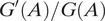
. It is plausible, however, that successful revolts may require a critical mass of attackers, meaning that the success determination technology may exhibit increasing and then decreasing returns. Our assumption can accommodate this type of success determination technology because log-concavity is consistent with increasing returns as long as
 $ {G}^{\prime }(A)/G(A) $
is nonincreasing. The second part of our assumption (i.e.,
 $ G(0)>{c}_f/{k}_f $
) is a sufficient condition that guarantees the existence of nontrivial equilibria with a positive mass of attackers. This condition requires that
 $ G(0) $
be positive. A regime facing mass discontent may implode or collapse due to many forces (e.g., internal strife among elites, economic pressure, or foreign intervention) other than the actions of revolutionary leaders and followers. We can interpret
 $ G(0) $
as the probability that these “background factors” bring down the regime.Footnote
13
In this game with asymmetric information, nature picks the state first. Then the leader observes the state and proposes an agenda. Citizens observe the agenda, make inferences about the state, and make participation decisions. Finally, the revolt can be a success or failure, depending on the mass of attackers and some random factors. The timeline of the game is summarized in Figure 1.
Timeline of the Game with Asymmetric Information

Equilibrium of the Protest Game
In the following, we solve the model backwards. We first deal with the last stage, where citizens correctly infer about the state from the agenda proposed by the opposition leader and decide to attack the regime or not, taking the agenda as given. We then analyze the agenda decision of the leader under full information and asymmetric information in the last two subsections.
Given the status quo policy
 $ {y}_0 $
and the reform agenda
 $ {y}_1 $
, citizens decide whether to attack the regime or not in a simple protest game when the state
 $ \theta $
is learned and becomes common knowledge. For any expected size of attack
 $ A $
, citizen
 $ i $
chooses
 $ {a}_i=1 $
, if and only if the follower’s premium (defined in the previous subsection)
 $ FP\left({x}_i;A,{y}_1\right)\ge 0 $
. The function
 $ FP\left(\cdot; A,{y}_1\right) $
is weakly increasing; therefore, there exists a marginal attacker, denoted
 $ {x}^f $
and satisfying
 $ FP\left({x}^f;A,{y}_1\right)=0 $
, such that citizen
 $ i $
attacks if and only if
 $ {x}_i\ge {x}^f $
. Figure 2 illustrates the determination of the marginal attacker
 $ {x}^f $
given a pair of policies
 $ {y}_0 $
and
 $ {y}_1 $
.
The Determination of the Marginal Attacker
 $ {x}^f $
.
Note: The utility difference between the solid line and the dashed line represents the reward from success for citizens with preference
 $ {x}_i $
. The follower’s premium is nonnegative if and only if
 $ {x}_i\ge {x}^f $
.

Under this decision rule and the uniform distribution assumption, the total mass of attackers is
 $ A=1-{x}^f $
. The equilibrium of the protest game can be characterized by the indifference condition for the marginal attacker, which can be written as
 $$ FP\left({x}^f;1-{x}^f,{y}_1\right)={k}_fG\left(1-{x}^f\right)\left(u\left({y}_1,\theta, {x}^f\right)-u\Big({y}_0,\theta, {x}^f\Big)\right)-{c}_f=0. $$
To emphasize its dependence on the reform agenda and the state, we use
 $ {x}^f\left({y}_1;\theta \right)\in \left(0,1\right) $
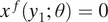
to denote the equilibrium marginal attacker that satisfies condition (2). If
 $ FP\left(0;1,{y}_1\right)\ge 0 $
, then
 $ {x}^f\left({y}_1;\theta \right)=0 $
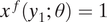
, and all citizens attack. If
 $ FP\left(1;0,{y}_1\right)<0 $
, then
 $ {x}^f\left({y}_1;\theta \right)=1 $
, and no one attacks.
Lemma 1.
There exists
 $ {y}_{\mathrm{min}}\left(\theta \right)\in \left({y}_0,1+\theta \right) $
such that (a) if
 $ {y}_1<{y}_{\mathrm{min}}\left(\theta \right) $
, then the only equilibrium is a no-attack equilibrium and (b) if
 $ {y}_1 \ge {y}_{\mathrm{min}}\left(\theta \right) $
, then there exists only one equilibrium with a positive mass of attackers and with
 $ {x}^f\left({y}_1;\theta \right) \le {y}_1-\theta $
. Further, in case (b), the mass of attackers increases when the agenda is less radical or when the state is higher.
In case (a) of Lemma 1, the reward from success is small if the reform agenda
 $ {y}_1 $
is close to the status quo
 $ {y}_0 $
. Given a positive cost of participation, no one chooses to participate in the movement. In case (b), the reform agenda
 $ {y}_1 $
is sufficiently far from the status quo, which guarantees at least a fraction of the relatively more radical citizens would find it worthwhile to attack—that is, a nontrivial equilibrium exists. In this case, there may be multiple equilibria, one with
 $ {x}^f\le {y}_1-\theta $
and another with
 $ {x}^f>{y}_1-\theta $
.Footnote
14 Throughout the paper, we focus on the equilibrium with the largest equilibrium attack size (i.e., the one with
 $ {x}^f\le {y}_1-\theta $
). This is the only interior equilibrium in which the cutoff strategy (i.e., attack if and only if
 $ {x}_i \ge {x}^f $
) can be reasonably justified, and it is stable with meaningful comparative statics.
In a nontrivial equilibrium of the protest game, a more radical reform agenda
 $ {y}_1 $
suppresses participation. First, because
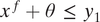 $ {x}^f+\theta \le {y}_1 $
, the reform agenda is already to the right of the ideal policy of the marginal attacker. Raising
 $ {y}_1 $
further would make the agenda even less appealing to this citizen. Thus, holding
 $ A $
fixed, the marginal attacker shifts to the right. Second, as fewer citizens participate (i.e.,
 $ A $
decreases), the follower premium falls for every citizen, which shifts the marginal attacker to the right even further. Consequentially, the marginal attacker becomes more radical and the probability of success falls correspondingly.
Equally important, a larger mismatch between the state and status quo policy causes more citizens to prefer the proposed policy
 $ {y}_1 $
to the status quo
 $ {y}_0 $
because the reward from success is increasing in the state
 $ \theta $
for any
 $ {y}_1>{y}_0 $
. Lemma 1 shows that the size of the attack is larger when
 $ \theta $
is higher, which implies that the probability of success,
 $ G\left(1-{x}^f\left({y}_1;\theta \right)\right) $
, increases in
 $ \theta $
. Such a comparative static is particularly useful when the agenda decision is analyzed.
Strategic Reform Agenda in the Full-Information Benchmark
Now we turn to the agenda-making stage. The crux of our theory is that the agenda proposed by the leader has the dual role of informing citizens about the state and laying down a policy alternative that matters for their welfare after the regime change. In this section, we study a benchmark case in which we disentangle the informational role from the material role of the agenda by assuming that the state is known even before the leader announces the agenda. The results obtained will be utilized and contrasted with those obtained in the subsequent section, where the effect of asymmetric information is studied.
When the state
 $ \theta $
is common knowledge, the leader simply chooses
 $ {y}_1 $
to maximize her own payoff
 $ {U}_l\left({x}^m\right) $
, taking into account its influence on the protest game, characterized in Lemma 1. The leader’s maximization problem can be written as
 $$ \underset{y_1}{\max} u\left({y}_0,\theta, {x}^m\right)+\kappa G\left(1-{x}^f\left({y}_1;\theta \right)\right)\left[u\left({y}_1,\theta, {x}^m\right)-u\Big({y}_0,\theta, {x}^m\Big)\right]-{c}_l, $$
where
 $ \kappa =1+{k}_f+{k}_l $
if she chooses to attack in the protest game and
 $ \kappa =1+{k}_l $
if she chooses not to attack.
We restrict our attention to the interesting case where the leader’s ideal policy is large enough (i.e.,
 $ {x}^m+\theta >{y}_{\mathrm{min}} $
).Footnote
15 The leader would never find it optimal to choose an agenda that is more radical than her ideal policy (i.e.,
 $ {y}_1>{x}^m+\theta $
) because she can always choose a less radical policy that is closer to her ideal policy and that gives rise to a higher probability of success. She would not choose a very moderate agenda, either (i.e.,
 $ {y}_1<{y}_{\mathrm{min}} $
), because such an agenda would induce no attack in the protest game. For
 $ {y}_1\in \left[{y}_{\mathrm{min}},{x}^m+\theta \right] $
, the objective function (3) is quasiconcave; therefore, the optimal agenda
 $ {y}_1^{\ast } $
is unique and is characterized by the first-order condition. We also show that it is not optimal to choose
 $ {y}_1={y}_{\mathrm{min}} $
. The optimal agenda
 $ {y}_1^{\ast } $
satisfies
 $$ 1-\frac{G^{\prime}\left(1-{x}^f\left({y}_1^{\ast };\theta \right)\right)}{G\left(1-{x}^f\left({y}_1^{\ast };\theta \right)\right)}\frac{\partial {x}^f\left({y}_1^{\ast };\theta \right)}{\partial {y}_1}\left({y}_1^{\ast }-{y}_0\right)\ge 0, $$
with
 $ {y}_1^{\ast }={x}^m+\theta $
if (4) holds as a strict inequality.
The leader faces a trade-off between the reward from success and the chances of success. The marginal utility from having a policy closer to the leader’s ideal policy is
 $ 1 $
. The marginal cost is that the chance of obtaining the reward from success is lowered as
 $ \partial {x}^f/\partial {y}_1 $
is positive by Lemma 1. The first-order condition (4) optimally balances this trade-off. Because this optimal agenda
 $ {y}_1^{\ast } $
reflects the leader’s concern about the equilibrium outcome in the subsequent protest game, we sometimes refer to it as a strategic agenda, and we write
 $ {y}_1^{\ast}\left({x}^m;\theta \right) $
to emphasize its dependence on the leader’s preference and on the state.
Proposition 1.
For any leader with
 $ {x}^m\ge {y}_{\mathrm{min}}\left(\theta \right)-\theta $
, there exists a unique cutoff
 $ \hat{x}\left(\theta \right) $
such that the strategic agenda is
 $$ {y}_1^{\ast}\left({x}^m;\theta \right)=\left\{\begin{array}{cc}{x}^m+\theta & if\;{x}^m<\hat{x}\left(\theta \right);\\ {}\hat{x}\left(\theta \right)+\theta & if\;{x}^m\ge \hat{x}\left(\theta \right).\end{array}\right. $$
Further, a higher state makes the strategic agenda more radical, but increases the probability of success in the protest game.
When the leader’s preference
 $ {x}^m $
is relatively moderate (i.e.,
 $ {x}^m<\hat{x}\left(\theta \right) $
), she can afford to choose her own ideal policy (i.e.,
 $ {x}^m+\theta $
) without suppressing citizens’ support very much—that is, the optimal solution
 $ {y}_1^{\ast}\left({x}^m;\theta \right) $
is a corner solution. When the leader’s preference is relatively radical (i.e.,
 $ {x}^m\ge \hat{x}\left(\theta \right) $
), choosing her ideal policy would discourage too many moderate citizens from joining the mass movement. Therefore, the leader must compromise by choosing the agenda
 $ {y}_1^{\ast }=\hat{x}\left(\theta \right)+\theta $
, which is less radical than her ideal policy. In general, the strategic agenda
 $ {y}_1^{\ast}\left({x}^m;\theta \right) $
is weakly increasing in
 $ {x}^m $
.Footnote
16
The second part of the proposition says that the opposition leader chooses a more radical agenda in response to a higher state, but would never raise the equilibrium agenda
 $ {y}_1^{\ast } $
to the point where it hurts the chances of success. In other words,
 $ G\left(1-{x}^f\left({y}_1^{\ast}\left({x}^m;\theta \right);\theta \right)\right) $
always increases in
 $ \theta $
. In connection to the two states specified in our model, we let
 $ {y}_1^{L\ast} := {y}_1^{\ast}\left({x}^m;{\theta}_L\right) $
and
 $ {y}_1^{H\ast} := {y}_1^{\ast}\left({x}^m;{\theta}_H\right) $
represent the strategic agenda chosen by the leader with preference
 $ {x}^m $
in the low and high states, respectively, under full information. Further, let
 $ {G}^{L\ast} := G\left(1-{x}^f\left({y}_1^{L\ast };{\theta}_L\right)\right) $
and
 $ {G}^{H\ast} := G\left(1-{x}^f\left({y}_1^{H\ast };{\theta}_H\right)\right) $
represent the corresponding probabilities of success. Proposition 1 states that
 $ {y}_1^{H\ast }>{y}_1^{L\ast } $
and
 $ {G}^{H\ast }>{G}^{L\ast } $
.
The implication of this result is important for our subsequent analysis. Once citizens believe that the environment is more favorable for a revolt (i.e., the state is high), the leader can choose a more radical agenda, but the chances of success are also greater. That provides the leader an incentive to mislead citizens when the leader knows the state but citizens do not know. In the next section, such an incentive will be the focus of our analysis. We will also show that, under some circumstances, asymmetric information may cause the leader to “overreact”: she chooses a policy so radical that it reduces the probability of success, despite the state being more favorable to the mass movement.
Radical Reform Agenda in Separating Equilibrium
In this section, we analyze the case of asymmetric information, in which only the leader knows the state but citizens do not. In this setting, the leader lacks an effective means of convincing citizens that it is her information rather than her own interest that drives her choice of agenda. She has to rely on the reform agenda to credibly signal her private information. Such a signaling mechanism is costly, because the agenda has to be distorted to command credibility.
In the following formal analysis, we restrict our attention to leaders with a preference higher than a threshold (specifically,
 $ {x}^m\ge {y}_{\mathrm{min}}\left({\theta}_L\right)-{\theta}_L $
) to ensure that in each state, there is a positive mass of attackers in the equilibrium of the protest game.
Lemma 2.
There exists a unique threshold
 $ {x}^{\dagger}\in \left(\hat{x}\left({\theta}_H\right),\hat{x}\left({\theta}_H\right)+{\theta}_H-{\theta}_L\right) $
such that the full-information outcome
 $ \left({y}_1^{L\ast },{y}_1^{H\ast}\right) $
is an equilibrium outcome under asymmetric information if and only if the leader is moderate, i.e.,
 $ {x}^m\le {x}^{\dagger } $
.
The leader in the low state may have an incentive to mislead citizens into believing that the state is high, and the more radical her preference is, the greater the incentive to mislead. First, for the same reform agenda, the mass of attackers is larger if citizens believe that the state is high (Lemma 1) when it is actually low. Second, when the leader misleads citizens with
 $ {y}_1^{H\ast } $
, the reward from success could be either larger or smaller, depending on whether
 $ {y}_1^{H\ast } $
or
 $ {y}_1^{L\ast } $
is closer to her ideal policy. Specifically, by choosing
 $ {y}_1^{H\ast } $
instead of
 $ {y}_1^{L\ast } $
in the low state, the reward from success would change from
 $ {y}_1^{L\ast }-{y}_0 $
to
 $ 2{x}^m+2{\theta}_L-{y}_1^{H\ast }-{y}_0 $
. For a leader with low
 $ {x}^m $
, the policy
 $ {y}_1^{H\ast } $
is too far from her ideal policy in the low state, and the net change is negative. For a leader with high
 $ {x}^m $
, the policy
 $ {y}_1^{H\ast } $
can be closer to her ideal policy in the low state, and the net change is positive. In general, the net change is larger when the leader is more radical. Therefore, in the low state
 $ {\theta}_L $
, a leader with a moderate preference (small
 $ {x}^m $
) faces a trade-off between a higher chance of success and a lower reward from success when she lies. However, both are higher for a leader with a radical preference (large
 $ {x}^m $
). Lemma 2 shows that there exists a unique
 $ {x}^{\dagger } $
such that the concern over a lower reward dominates the benefit of a higher chance of success if and only if
 $ {x}^m\le {x}^{\dagger } $
. We say that the leader is moderate if
 $ {x}^m\le {x}^{\dagger } $
and radical, otherwise.
Suppose the leader’s preference is moderate (
 $ {x}^m\le {x}^{\dagger } $
); she thus has no incentive to mislead, and citizens know this. In equilibrium, the leader would choose the strategic agenda
 $ {y}_1^{L\ast } $
in the low state and the strategic agenda
 $ {y}_1^{H\ast } $
in the high state, and citizens correctly infer about the state. In other words, the leader indeed behaves “optimally”—that is, as she would behave under full information.
Suppose the leader’s preference is radical (
 $ {x}^m>{x}^{\dagger } $
); she thus has an incentive to mislead by proposing
 $ {y}_1^{H\ast } $
in the low state. Of course, citizens would not be fooled into believing that the state is high simply because they observe the leader choosing the reform agenda
 $ {y}_1^{H\ast } $
. In this case, the full-information outcome cannot be supported as an equilibrium outcome under asymmetric information. In the following proposition, we characterize the least-cost separating equilibrium that satisfies the D1 criterion (Banks and Sobel Reference Banks and Sobel1987; Cho and Kreps Reference Cho and Kreps1987). We show that the agenda chosen must be even more radical than
 $ {y}_1^{H\ast } $
in the high state, so the leader would not have an incentive to mimic the high state by choosing this very radical policy when the state is low. In other words, the radical leader cannot behave “optimally” in the high state; she has to resort to “irrational radicalism” to separate herself from leaders who may otherwise bluff in order to boost support.
To formalize, let
 $ ({\hat{y}}_1^L,{\hat{y}}_1^H) $
represent the agenda choices in the separating equilibrium in the respective states. Let
 $ {\hat{G}}^L := G(1-{x}^f({\hat{y}}_1^L;{\theta}_L)) $
and
 $ {\hat{G}}^H := G(1-{x}^f({\hat{y}}_1^H;{\theta}_H)) $
represent the corresponding probabilities of success.
Proposition 2.
Suppose the leader is radical (i.e.,
 $ {x}^m>{x}^{\dagger } $
). In the least-cost separating equilibrium that satisfies the D1 refinement, compared with the full-information benchmark, we have the following: (i) in the low state, the equilibrium agenda remains the same (i.e.,
 $ {\hat{y}}_1^L={y}_1^{L\ast } $
and
 $ {\hat{G}}^L={G}^{L\ast } $
) and (ii) in the high state, the equilibrium agenda is more radical and chances of success are lower (i.e.,
 $ {\hat{y}}_1^H>{y}_1^{H\ast } $
and
 $ {\hat{G}}^H<{G}^{H\ast } $
). Further, (iii) as the leader’s preference
 $ {x}^m $
is more radical, the agenda
 $ {\hat{y}}_1^H $
is strictly more radical.
Part (i) says that, in a separating equilibrium, the leader would not propose an agenda different from
 $ {y}_1^{L\ast } $
in the low state. Any agenda other than optimal strategic policy would give her a lower payoff as long as the low state is correctly inferred by citizens.
Part (ii) establishes a contrasting result in the high state. For any leader with
 $ {x}^m>{x}^{\dagger } $
, proposing an agenda equal to
 $ {y}_1^{H\ast } $
in the high state will not be an equilibrium (Lemma 2). To prevent her from overstating the favorability of the state, the equilibrium policy
 $ {\hat{y}}_1^H $
must exceed
 $ {y}_1^{H\ast } $
.Footnote
17 Such an equilibrium agenda is so high that it is to the right of the leader’s ideal policy
 $ {x}^m+{\theta}_L $
in the low state, and it significantly reduces the probability of success, which makes proposing
 $ {\hat{y}}_1^H $
unattractive in the low state. In other words, in the high state, to convince citizens of the state, a radical leader must pursue a policy that is too radical and too costly at the expense of losing too many followers.
The reform agenda in the high state under the least-cost separating equilibrium that satisfies the D1 refinement is the
 $ {\hat{y}}_1^H $
(greater than
 $ {y}_1^{H\ast } $
) such that the leader’s incentive constraint in the low state is just binding:
 $$ {\hat{G}}^L(u({\hat{y}}_1^L,{\theta}_L,{x}^m)-u({y}_0,{\theta}_L,{x}^m\Big))-{\hat{G}}^H(u({\hat{y}}_1^H,{\theta}_L,{x}^m)-u({y}_0,{\theta}_L,{x}^m\Big))=0. $$
When the leader is indifferent between
 $ {\hat{y}}_1^L $
and
 $ {\hat{y}}_1^H $
in the low state, she strictly prefers
 $ {\hat{y}}_1^H $
to
 $ {\hat{y}}_1^L $
in the high state.Footnote
18 Figure 3 illustrates the equilibrium outcome.
Strategic Agenda and Radical Agenda.
Note: The strategic agenda pair is
 $ \left({y}_1^{L\ast },{y}_1^{H\ast}\right) $
under full information. When
 $ {x}^m>{x}^{\dagger } $
, the leader chooses
 $ {\hat{y}}_1^L={y}_1^{L\ast } $
and
 $ {\hat{y}}_1^H>{y}_1^{H\ast } $
in a separating equilibrium, and
 $ {\hat{y}}_1^H $
strictly increases in
 $ {x}^m $
.

In the least-cost separating equilibrium, the chance of success in the high state must be lower than that in the full-information setting (i.e.,
 $ {\hat{G}}^H<{G}^{H\ast } $
). That is because the reform agenda in the high state is more radical, and the mass of attackers decreases with a more radical agenda (Lemma 1). In the high state, the leader cannot moderate her position, even though she knows that her radical agenda discourages citizens: citizens would interpret an agenda less radical than
 $ {\hat{y}}_1^H $
as an opportunistic deviation by a leader who attempts to exaggerate the state by choosing a high agenda in the low state.
Part (iii) of Proposition 2 characterizes the comparative statics of the equilibrium
 $ {\hat{y}}_1^H $
with respect to
 $ {x}^m $
. As the leader becomes more radical, her incentive to exaggerate the state and mislead citizens increases. As a result, she needs to propose even more radical agendas in the high state in order to remain credible. Interestingly, when the leader is very radical, the more favorable state does not necessarily guarantee a better chance of success because the agenda chosen to signal the state is too radical.
A corollary to Proposition 2 is that there exists
 $ {x}^{\dagger \dagger }>{x}^{\dagger } $
such that, if the leader’s preference is more radical than
 $ {x}^{\dagger \dagger } $
, then the chances of success are smaller in the high state than in the low state. Because
 $ {\hat{y}}_1^H $
increases with
 $ {x}^m $
at a nonvanishing rate for a large enough
 $ {x}^m $
, and
 $ {\hat{y}}_1^L $
is constant with respect to
 $ {x}^m $
for
 $ {x}^m>\hat{x}\left({\theta}_L\right) $
, we must have
 $ {\hat{y}}_1^H-2{\theta}_H>{\hat{y}}_1^L-2{\theta}_L $
when
 $ {x}^m $
exceeds a threshold value
 $ {x}^{\dagger \dagger } $
. By the indifference condition (2) for the marginal attacker, this inequality implies that
 $ {x}^f\left({\hat{y}}_1^H;{\theta}_H\right)>{x}^f\left({\hat{y}}_1^L;{\theta}_L\right) $
, and hence
 $ {\hat{G}}^H<{\hat{G}}^L $
. Such an equilibrium outcome under asymmetric information is qualitatively different from that under full information, where we show that
 $ {G}^{H\ast }>{G}^{L\ast } $
. That is, the leader who does not suffer from the citizens’ suspicion always proposes a more radical agenda given a higher state, but she never “overreacts” by choosing a policy so radical that it hurts the chances of success.
Endogenous Leadership
In the previous section, we showed that a radical leader may have to radicalize her agenda to signal that she is not lying to gather support, while a moderate leader is not plagued by such suspicion. A relevant question is, under what conditions would radicals rather than moderates assume the leadership role and propose the reform agenda? Before dealing with this question, one must acknowledge that there can be plenty of plausible routes to opposition leadership, including by sheer chance in many historical events. In this section, we analyze one particular mechanism of how the leadership of a movement may endogenously emerge: citizens can choose to join the leadership, and a reform agenda is proposed as a compromise among leaders with diverse interests. Interestingly, this mechanism of leadership selection and the mechanism of signaling reinforce each other, which, under some circumstances, produces an equilibrium outcome whereby radicals indeed become leaders.
Leader Selection
We enrich the model in the previous section by allowing the opposition leadership to comprise a group of citizens instead of a single leader and by making the choice to join the leadership group endogenously. Specifically, before observing the state, each citizen only knows its distribution and can make an additional decision to join the leadership of the mass movement (
 $ {l}_i=1 $
) or not (
 $ {l}_i=0 $
). In each state, the payoff to any citizen who chooses to be a leader is given by Equation 1.Footnote
19
If no citizens choose to join the leadership, then the status quo will prevail, and therefore there will be no revolt. If a group of citizens decide to join the leadership, their preferences within the leadership group must be diverse. We assume that it is the one with the median preference among the leadership group who will formulate and propose the reform agenda for the mass movement. In other words, the task of drafting the policy proposal is delegated to the median citizen in the group, who will be referred to as the median leader in the following. We continue to use
 $ {x}^m $
to denote the preference of the median leader.
Citizens choose to join the leadership before they know the state. After the median leader emerges from the leadership group, she observes the state, makes a proposal, and announces it to all the other citizens. Upon hearing the proposal, each citizen makes inferences about the state and decides whether to participate in attacking the regime or not. That is, once the median leader acquires information about the state, the rest of the game is similar to the benchmark model. The timing of the game with endogenous leadership is summarized in Figure 4. The equilibrium of this static game is a fixed point, in which the preference of the median leader is endogenously determined and known to other citizens.
Timeline of the Game with Asymmetric Information and Endogenous Leadership

The assumptions related to the emergence of leaders deserve discussion. First, the assumption that the median leader chooses the agenda captures the idea that the proposed agenda should reflect the preferences of the leadership group as a whole. This can be formally justified by a democratic decision-making process within the leadership group, in which the median leader’s preference prevails in any pairwise vote between reform agendas. This assumption appears to be rather specific but is a useful shortcut for representing two general conditions: (i) the policy proposed by the leadership group is more radical than the policy preferred by the least radical leader in the group and (ii) the proposed policy becomes more radical if a fraction of the least radical leaders are removed from the group. Conceptually, the precise policy formulation mechanism matters little for the subsequent analysis and results, as long as conditions (i) and (ii) hold, but our setting is more tractable.Footnote 20
Second, in this model, there will be a continuum of leaders. Only the median leader chooses the agenda; what she proposes affects the payoffs of all leaders but not the other way around because each leader is atomistic and her decision to become a leader or not has no influence on who will be selected as the median leader. This assumption is made to simplify the characterization. Even in a setting with a finite number of leaders, the agenda-making mechanism can still satisfy conditions (i) and (ii), in which case our results and analysis continue to hold.Footnote 21
Finally, regarding the timing, we assume that citizens do not observe the state before they choose to join the leadership, which is reasonable but not crucial for our results. This is reasonable because political mass movements are often sudden outbreaks, and individuals who become leaders may acquire information about the political situation after they assume their role.Footnote 22 It is not crucial, because we can also allow a small fraction of randomly drawn citizens to observe the state before they decide whether to participate in the leadership group. In a separating equilibrium where the rest of citizens still infer the state from the reform agenda, the main results and properties of leadership formation will be similar.
Equilibrium Analysis
Because citizens do not know the state at the time that they choose to become leaders, the determination of endogenous leadership is based on the expected value of the leader’s premium. Specifically, if the preference of the median leader is conjectured to be equal to
 $ {x}^m $
, citizens expect that the proposed agenda is
 $ {\hat{y}}_1^L\left({x}^m\right) $
or
 $ {\hat{y}}_1^H\left({x}^m\right) $
, depending on the state. The expected leader’s premium for a citizen with preference
 $ {x}_i $
is
 $$ \hat{L}P\left({x}_i;{x}^m\right) := \sum \limits_{j=L,H}{\pi}_j LP\left({x}_i;{\hat{y}}_1^j\left({x}^m\right),{\theta}_j\right), $$
where
 $$ LP\left({x}_i;{y}_1,\theta \right)=\left\{\begin{array}{cc}{k}_lG\left(1-{x}^f\left({y}_1;\theta \right)\right)\left(2{x}_i+2\theta -{y}_1-{y}_0\right)-{c}_l& \mathrm{if}\;{x}_i+\theta <{y}_1,\\ {}{k}_lG\left(1-{x}^f\left({y}_1;\theta \right)\right)\left({y}_1-{y}_0\right)-{c}_l & \mathrm{if}{x}_i+\theta \ge {y}_1.\end{array}\right. $$
For a given
 $ {x}^m $
, citizen
 $ i $
chooses to join the leadership group if and only if the expected leader’s premium is nonnegative. Since
 $ LP\left({x}_i;{y}_1,\theta \right) $
is weakly increasing in
 $ {x}_i $
,
 $ \hat{L}P\left({x}_i;{x}^m\right) $
is also weakly increasing in
 $ {x}_i $
, which justifies a monotone strategy. That is, if there exists a marginal leader
 $ {x}^l $
such that
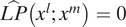 $ \hat{L}P\left({x}^l;{x}^m\right)=0 $
, then citizen
 $ i $
chooses
 $ {l}_i=1 $
if and only if
 $ {x}_i\ge {x}^l $
. If
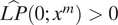 $ \hat{L}P\left(0;{x}^m\right)>0 $
, then all citizens choose to become leaders, and if
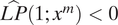 $ \hat{L}P\left(1;{x}^m\right)<0 $
, then no citizen chooses to be a leader. Of course, the preference of the marginal leader depends on
 $ {x}^m $
, and we write
 $ {x}^l\left({x}^m\right) $
to emphasize this dependence.
Because the distribution of preferences
 $ {x}_i $
is uniform, if the marginal leader has preference
 $ {x}^l\left({x}^m\right) $
, then the median preference of the leadership group is
 $$ M\left({x}^m\right)=\frac{1}{2}\left({x}^l\left({x}^m\right)+1\right). $$
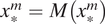
The equilibrium in this model is characterized by a 6-tuple,
 $ \left({x}_{\ast}^m,{x}_{\ast}^l,{x}_{L\ast}^f,{x}_{H\ast}^f,{\hat{y}}_{1\ast}^L,{\hat{y}}_{1\ast}^H\right) $
, that satisfies the following requirements:
-
1. The median leader’s preference satisfies
 $ {x}_{\ast}^m=M\left({x}_{\ast}^m\right) $
.
-
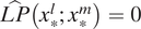
2. The marginal leader’s preference satisfies
$ \hat{L}P\left({x}_{\ast}^l;{x}_{\ast}^m\right)=0 $
. -
3. The reform agenda in the low state solves the maximization problem (3) and is given by
$ {\hat{y}}_{1\ast}^L={y}_1^{\ast}\left({x}_{\ast}^m;{\theta}_L\right) $
in Equation 5. -
4. If
$ {x}_{\ast}^m\le {x}^{\dagger } $
, the reform agenda is given by
$ {\hat{y}}_{1\ast}^H={y}_1^{\ast}\left({x}_{\ast}^m;{\theta}_H\right) $
in Equation 5; otherwise, it is given by the solution to the binding incentive constraint (6) for
$ {x}^m={x}_{\ast}^m $
and
$ {\hat{y}}_1^L={\hat{y}}_{1\ast}^L $
. -
5. The marginal attacker in state
$ j\in \left\{H,L\right\} $
satisfies
$ FP\left({x}_{j\ast}^f;1-{x}_{j\ast}^f,{\hat{y}}_{1\ast}^j,{\theta}_j\right)=0 $
.






In this equilibrium, citizen
 $ i $
chooses
 $ {l}_i=1 $
if and only if
 $ {x}_i\ge {x}_{\ast}^l $
, and she chooses
 $ {a}_i=1 $
in state
 $ j\in \left\{H,L\right\} $
if and only if
 $ {x}_i\ge {x}_{j\ast}^f $
. The probability of success in state
 $ j $
is
 $ G\left(1-{x}_{j\ast}^f\right) $
.
The key to our model is that the leadership premium
 $ \hat{L}P\left({x}_i;{x}^m\right) $
is weakly increasing in
 $ {x}_i $
, and any citizen with preference
 $ {x}_i\ge {x}^l\left({x}^m\right) $
will choose to be a leader. That means that the median leader
 $ {x}^m $
in general is more radical than the marginal leader
 $ {x}^l $
(i.e., condition (i) holds), and the median leader
 $ {x}^m $
is more radical if the marginal leader
 $ {x}^l $
is more radical (i.e., condition (ii) holds).
The two conditions combined give rise to a mechanism for the determination of the leadership, in which the mapping
 $ M\left({x}^m\right) $
is increasing in
 $ {x}^m $
. To understand the positive slope, consider the following comparative statics on an increase in the preference of the median leader (i.e., a larger
 $ {x}^m $
). The median leader would propose more radical agendas—that is,
 $ {\hat{y}}_1^L\left({x}^m\right) $
and
 $ {\hat{y}}_1^H\left({x}^m\right) $
are both higher (Propositions 1 and 2), and this, in turn, hurts the marginal leader who has less radical preferences than the median one. As a result, a more radical citizen would become the marginal leader—that is,
 $ {x}^l\left({x}^m\right) $
shifts to the right as
 $ {x}^m $
increases. The distribution of preferences of the leadership group therefore becomes more radical, which, consequentially, gives rise to a more radical median leader. In other words, the leadership group will be more radical if the conjectured median leader becomes more radical. The solid line in Figure 5 illustrates the mapping
 $ M\left({x}^m\right) $
.
Proposition 3.
Under some sufficient conditions guaranteed by neither
 $ {c}_f/{k}_f $
nor
 $ {c}_l/{k}_l $
being too large, the mapping
 $ M\left(\cdot \right) $
is continuous and increasing on
 $ \left[1/2,1\right] $
, and there exists an equilibrium with
 $ {x}_{\ast}^m\in \left(1/2,1\right) $
such that a positive mass of citizens choose to attack in each state. Further, if
 $ {\theta}_H-{\theta}_L\le 1/3 $
, the equilibrium is unique.
Fixed Point.
Note: The solid black curve represents
 $ M\left({x}^m\right) $
, and
 $ {x}_{\ast}^m $
is the fixed point. When the cost of joining the leadership is higher,
 $ M\left({x}^m\right) $
shifts up and the equilibrium
 $ {x}_{\ast}^m $
increases.

To ensure the existence of a nontrivial equilibrium in the protest game, we require that
 $ {c}_f/{k}_f $
be smaller than a threshold.Footnote
23 To ensure that the leadership is not empty in equilibrium, we require that
 $ {c}_l/{k}_l $
be smaller than a threshold so that a citizen with preference
 $ {x}_i\in \left[1/2,1\right] $
will choose to be a leader if she expects herself to be the median leader who proposes the reform agendas.Footnote
24 Under these conditions, Proposition 3 establishes that
 $ M\left({x}^m\right) $
is increasing and that a fixed point of the mapping exists.
The fixed point of
 $ M\left(\cdot \right) $
is unique and stable if its slope is less than one. Intuitively,
 $ {M}^{\prime}\left({x}^m\right) $
will be smaller if fewer leaders on the left end of the leadership drop out when the median leader becomes more radical. This is true when the proposed policy
 $ {\hat{y}}_1^H\left({x}^m\right) $
does not increase too much when the leader’s preference
 $ {x}^m $
becomes more radical. Proposition 3 shows that the condition
 $ {\theta}_H-{\theta}_L\le 1/3 $
is sufficient to ensure that
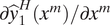 $ \partial {\hat{y}}_1^H\left({x}^m\right)/\partial {x}^m $
is so small that the slope of
 $ M\left(\cdot \right) $
is less than one. Therefore, the fixed point is also a globally stable one: convergence to the fixed point from any likely perturbations is guaranteed.
We have characterized the determination of the endogenous leadership group. In the following section, we investigate the conditions under which citizens with radical preferences take on the leadership roles and how this mechanism of leadership selection and the mechanism of signaling reinforce each other.
Discussion
Suppression and the Opposition Leadership
Facing the challenge of mass movements, regimes typically resort to harsher punishments to thwart the revolts, which may secure a higher chance of regime survival but may also radicalize the opposition leadership. Therefore, successful revolts can be less likely but more radical. This observation is consistent with the comparative statics of our model: a greater suppression of the mass movement by the regime may radicalize the leadership in equilibrium (i.e., the preference of the leader
 $ {x}_{\ast}^m $
may rise above
 $ {x}^{\dagger } $
, in response to harsher punishments), and the radical leader is therefore compelled to radicalize her agenda out of the signaling concern.
Consider first an increase in the cost of joining the leadership
 $ {c}_l/{k}_l $
, which reflects the harsher punishment imposed by the regime targeting leaders specifically. Other things being equal, a higher
 $ {c}_l/{k}_l $
reduces the leader’s premium and causes the marginal (and moderate) leaders to drop out. As the preference of the marginal leader
 $ {x}^l $
increases, the preference of the median leader of the remaining group,
 $ \left({x}^l+1\right)/2 $
, also increases. In Figure 5, the curve representing
 $ M\left({x}^m\right) $
shifts up from the solid line to the dashed line. In the new equilibrium, a more radical leader will be chosen, and the agendas chosen in both states will be more radical as well.
This result is consistent with a common conjecture about radicalism from the perspective of leader selection: high costs of leading movements filter out moderates, and only radicals remain. In addition, our model shows that the impact of higher
 $ {c}_l/{k}_l $
on the selection of leaders is amplified through the endogenous selection of leaders, which is absent in the aforementioned conjecture. This discussion also highlights why it is important to introduce an endogenous mechanism to determine leadership in our model. When the leader is exogenous and imposed, the cost of leadership does not matter for the equilibrium agendas. When citizens can choose to join the leadership or not, such a cost becomes important because it helps determine how radical the leadership group is.
Consider next an increase in the cost of participating in the protests
 $ {c}_f/{k}_f $
, which reflects the harsher punishment imposed by the regime targeting all participants. A higher participation cost gives rise to two effects. The direct effect is that fewer followers join the movement, reducing the chances of success and hence the expected payoff to the marginal leader. Therefore, the more moderate marginal leaders drop out and the median leader becomes more radical. The indirect effect is that for a fixed
 $ {x}^m $
, the median leader responds to lower participation by adjusting her strategic reform agenda. In particular, she may propose a more moderate agenda to partially compensate for the reduced chances of success, which benefits the marginal leader. The overall effect is theoretically ambiguous. However, for a large set of parameters, we find that the direct effect dominates the indirect effect: an increase in participation cost
 $ {c}_f/{k}_f $
leads to a more radical leadership group in equilibrium.Footnote
25
The above comparative statics result is consistent with one popular view about why the leadership of democracy movement of China in 1989 further radicalized, after the Chinese regime imposed martial law, which raised the cost of all participants. According to Ogden et al. (Reference Ogden, Hartford, Sullivan and Zweig1992, 123), “only those willing to risk everything for a political cause would come forth for leadership. Inevitably, this meant that the more radical, more daring students would, at each crucial juncture, control the course of the student movement, and move it onto ever more precarious ground.”
The new mechanism characterized in this section enriches the literature about the relationship between state repression and protests. On one hand, the direct influence of harsher punishments on radicalization of opposition leadership in this model corresponds to “the short term effect” found empirically in Rasler (Reference Rasler1996) that state repression discourages followers from participating in the Iran revolution. On the other hand, Rasler (Reference Rasler1996) shows that there exists an indirect effect that state repression increases protests through spatial diffusion. Our model also characterizes a similar indirect effect but through a different mechanism—the leader responds to lower participation by strategically adjusting her reform agenda. It is likely that the strength of two opposing effects varied in different settings: while state repression triggered overall larger protests in the context of the Iran revolution, repressive measures might have radicalized the leadership of democracy movement of China in 1989.Footnote 26
Structural Roots Hypothesis
In this section, we turn to the comparative statics of equilibrium outcomes with respect to
 $ {\pi}_H $
, the probability of favorable state for a revolt. We show that how
 $ {\pi}_H $
affects the equilibrium chances of success depends on whether the median leader is moderate or radical. Such a comparison is particularly interesting, because predictions of the model are qualitatively different if
 $ {x}_{\ast}^m<{x}^{\dagger } $
(with the leader choosing her agenda strategically) than if
 $ {x}_{\ast}^m>{x}^{\dagger } $
(with the leader “irrationally radicalizing” her agenda to signal the state).
If the equilibrium leader is moderate (i.e.,
 $ {x}_{\ast}^m \le {x}^{\dagger } $
), then an increase in
 $ {\pi}_H $
reduces
 $ {x}_{\ast}^m $
and raises the chances of success in both states. Given a moderate leader, the adopted agendas in both states are the strategic ones—that is,
 $ {y}_1^{L\ast } $
and
 $ {y}_1^{H\ast } $
. The marginal leader obtains a larger leader’s premium in the high state than in the low state because both the reward from success and the chances of success are larger in the high state. Therefore, an increase in
 $ {\pi}_H $
raises her expected leader’s premium and encourages more citizens to become leaders, making the leadership group more moderate. Both the equilibrium
 $ {x}_{\ast}^l $
and
 $ {x}_{\ast}^m $
decrease in
 $ {\pi}_H $
. Further, the chances of success improve in both states because the equilibrium agendas become less radical. Panels (a) and (c) of Figure 6 illustrate.
Contrasting Comparative Statics with Respect to
 $ {\pi}_H $
When the Equilibrium Leader is Moderate Or Radical
Note: In this example, the success determination technology is
 $ G(A)=\Phi \left(1.5A-1\right) $
, where
 $ \Phi $
is the standard normal distribution function. The other parameters are:
 $ {y}_0=0 $
,
 $ {\theta}_L=0 $
,
 $ {\theta}_H=0.08 $
, and
 $ {c}_f/{k}_f=0.15 $
. In panels (a) and (c), we set
 $ {c}_l/{k}_l=0.1072 $
, and the leader is moderate in equilibrium. In panels (b) and (d), we set
 $ {c}_l/{k}_l=0.2573 $
, and the leader is radical in equilibrium.

In contrast, when the equilibrium leader is radical (i.e.,
 $ {x}_{\ast}^m>{x}^{\dagger } $
), such a prediction can be reversed: an increase in
 $ {\pi}_H $
raises
 $ {x}_{\ast}^m $
and reduces the chances of success in both states. Two conditions are sufficient for this reversed prediction: (i)
 $ {x}_{\ast}^m+{\theta}_L>{x}_{\ast}^l+{\theta}_H $
and (ii)
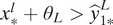 $ {x}_{\ast}^l+{\theta}_L>{\hat{y}}_{1\ast}^L $
. Condition (i) captures the situation that the interests of marginal and median leaders are sufficiently far apart. Together with the binding incentive constraint (6), this condition implies
 $$ {\hat{G}}^L\left({\hat{y}}_{1\ast}^L-{y}_0\right)={\hat{G}}^H\left(2{x}_{\ast}^m+2{\theta}_L-{\hat{y}}_{1\ast}^H-{y}_0\right)\ge {\hat{G}}^H\left(2{x}_{\ast}^l+2{\theta}_H-{\hat{y}}_{1\ast}^H-{y}_0\right). $$
Further, condition (ii) implies that
 $ {\hat{y}}_{1\ast}^L $
is to the left of the ideal policies of the marginal leader. Therefore, according to the definition of
 $ LP\left(\cdot \right) $
in the section on equilibrium analysis, the above inequality is equivalent to
 $ LP\left({x}_{\ast}^l;{\hat{y}}_{1\ast}^L,{\theta}_L\right)\ge LP\left({x}_{\ast}^l;{\hat{y}}_{1\ast}^H,{\theta}_H\right). $
This inequality says that the reform agenda in the high state is radicalized to such an extent that it is too far from the marginal leader’s ideal policy so that her leader’s premium in the high state is smaller than that in the low state. As a result, an increase in
 $ {\pi}_H $
(and a corresponding decrease in
 $ {\pi}_L $
) will reduce her expected leader’s premium. This will cause the marginal leader to drop out of the leadership, further causing
 $ M\left({x}^m\right) $
to increase as the remaining leaders become more radical. The equilibrium response is that
 $ {x}_{\ast}^m $
will rise. Therefore, both
 $ {\hat{y}}_{1\ast}^L $
and
 $ {\hat{y}}_{1\ast}^H $
are nondecreasing in
 $ {\pi}_H $
; the probabilities of success in both states are (weakly) smaller.
We illustrate the case of
 $ {x}_{\ast}^m>{x}^{\dagger } $
in panel (b) and (d) of Figure 6 by choosing a higher value of
 $ {c}^l/{k}^l $
than the one used in panels (a) and (c). In this example, conditions (i) and (ii) specified above are also satisfied. In such an equilibrium, the preference of the leader
 $ {x}_{\ast}^m $
increases in
 $ {\pi}_H $
, and the success probabilities in the two states weakly decreases. Observe also that
 $ {\hat{G}}^H<{\hat{G}}^L $
in this example: when the leader is very radical, the probability of success in the high state is lower than that in the low state.
This set of results also shed some new light on the debate about the role of structural factors in mass movements. The structural-roots hypothesis suggests that the fundamental social, economic, and political structures of society are the key determinants of the likelihood of regime change. In other words, mass political movements are more likely to succeed when society is riper for change. But Geddes (Reference Geddes1990) and Goldstone (Reference Goldstone2001) observe that in many societies that are plagued by structural roots of instability, upheavals with massive attacks do not occur, therefore calling into question the hypothesis.Footnote
27 But our analysis in this section shows that the probability of success may increase or decrease when the external environment is more favorable for revolt or riper for change (i.e.,
 $ {\hat{G}}^H $
can increase or decrease in
 $ {\pi}_H $
). Pooling these cases together without heeding the subtlety of the leadership’s role, an econometrician might conclude that the factors that can trigger political instability are observed more often than actual political upheavals themselves. According to our theory, it may be less puzzling than it appears.
Another line of critique of the structural roots hypothesis is that leaders’ characteristics matter for the outcome of political movements (Goldstone Reference Goldstone2001). Indeed, our work provides an example where leaders’ characteristics (i.e., their preferences for reform) matter. But we further demonstrate that structural factors may help determine who ends up playing the leadership role. Discussion in this section particularly highlights that both the punishment structure (i.e.,
 $ {c}_l/{k}_l $
and
 $ {c}_f/{k}_f $
) and the uncertain environment (i.e.,
 $ {\pi}_H $
) affect the leaders’ characteristics in equilibrium.
Conclusion
It is often said that desperate times call for desperate measures. The flip side to this is that desperate measures are a sign of desperate times. In this paper, we study how political leaders choose radical reform agendas as a signal to inform citizens that society badly needs to change. Our model goes beyond this basic insight, however. Specifically, moderate leaders are less inclined to radical ideals, which makes it easier for them to credibly convey their private information to the public. Radical leaders are known to prefer radical ideals; therefore, their claims and proposals are difficult to make credible even when their solutions are suitable for the situation. That helps explain why sometimes opposition leaders have to pursue very radical agendas even though they are aware that they will lose support. Although the focus of this paper is on radical reform agendas rather than radical tactics in social movements, with suitable modifications a similar logic can be applied to explain the latter as well. Further, to the best of our knowledge, our model is the first attempt to analyze explicitly the signaling role of radicalism and endogenous leadership in the context of collective actions.
Appendix
Proof of Lemma 1. For
 $ {y}_1\in \left[{y}_0,1+\theta \right] $
, define
 $$ \tilde{F}\left({y}_1\right) := FP\left({y}_1-\theta; 1-\left({y}_1-\theta \right),{y}_1\right)={k}_fG\left(1-\left({y}_1-\theta \right)\right)\left({y}_1-{y}_0\right)-{c}_f. $$
Log-concavity of
 $ G $
implies that
 $ \tilde{F} $
is quasiconcave. Since
 $ \tilde{F}\left({y}_0\right)<0 $
, and the assumption that
 $ G(0)>{c}_f/{k}_f $
implies
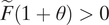 $ \tilde{F}\left(1+\theta \right)>0 $
, the function
 $ \tilde{F} $
must be single-crossing from below. Let
 $ {y}_{\mathrm{min}}\in \left({y}_0,1+\theta \right) $
represent such a crossing point. Because
 $ \tilde{F} $
must be increasing at the crossing point, we have
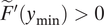 $ \tilde{F}\hbox{'}\left({y}_{\mathrm{min}}\right)>0 $
. Since
 $ \tilde{F} $
is quasiconcave,
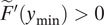 $ \tilde{F}\hbox{'}\left({y}_{\mathrm{min}}\right)>0 $
also implies
 $ \tilde{F}\hbox{'}\left({y}_1\right)>0 $
for all
 $ {y}_1<{y}_{\mathrm{min}} $
.
For
 $ {y}_1\in \left[{y}_0,1+\theta \right] $
and
 $ {x}^f\in \left[0,{y}_1-\theta \right] $
, define
 $$ F\left({x}^f;{y}_1\right) := FP\left({x}^f;1-{x}^f,{y}_1\right)={k}_fG\left(1-{x}^f\right)\left(2{x}^f+2\theta -{y}_1-{y}_0\right)-{c}_f. $$
Log-concavity of
 $ G $
again implies that
 $ F\left(\cdot; {y}_1\right) $
is quasiconcave. Moreover, it is easy to verify that
 $ \tilde{F}\hbox{'}\left({y}_1\right)>0 $
implies
 $ \partial F\left({x}^f;{y}_1\right)/\partial {x}^f>0 $
when evaluated at
 $ {x}^f={y}_1-\theta $
.
(a) Suppose
 $ {y}_1<{y}_{\mathrm{min}} $
. Since
 $ F\left(0;{y}_1\right)<0 $
and
 $ F\left({y}_1-\theta; {y}_1\right)=\tilde{F}\left({y}_1\right)<0 $
, and since
 $ \partial F\left({y}_1-\theta; {y}_1\right)/\partial {x}^f>0 $
, the quasiconcavity of
 $ F\left(\cdot; {y}_1\right) $
implies that
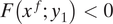 $ F\left({x}^f;{y}_1\right)<0 $
for any
 $ {x}^f\in \left[0,{y}_1-\theta \right] $
. For
 $ {x}^f>{y}_1-\theta $
, we have
 $$ FP\left({x}^f;1-{x}^f,{y}_1\right)={k}_fG\left(1-{x}^f\right)\left({y}_1-{y}_0\right)-{c}_f<\tilde{F}\left({y}_1\right)<0. $$
Because
 $ FP\left({x}^f;1-{x}^f,{y}_1\right)<0 $
for all
 $ {x}^f $
, the only equilibrium is one in which no one attacks.
(b) Suppose
 $ {y}_1\ge {y}_{\mathrm{min}} $
. Then we have
 $ F\left(0;{y}_1\right)<0 $
and
 $ F\left({y}_1-\theta; {y}_1\right)=\tilde{F}\left({y}_1\right)\ge 0 $
. Moreover, since
 $ F\left(\cdot; {y}_1\right) $
is quasiconcave in the relevant domain, it follows that there exists a unique
 $ {x}^f\in \left(0,{y}_1-\theta \right] $
that satisfies the equilibrium condition
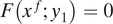 $ F\left({x}^f;{y}_1\right)=0 $
.
For the last part of the proposition, we let
 $ \lambda \left(\cdot \right) := {G}^{\prime}\left(\cdot \right)/G\left(\cdot \right) $
, and prove the following result.
Claim 1. For
 $ {y}_1\ge {y}_{\mathrm{min}}\left(\theta \right) $
,
 $$ {\displaystyle \begin{array}{c}\frac{\partial {x}^f}{\partial {y}_1}=\frac{k_fG\left(1-{x}^f\right)}{2{k}_fG\left(1-{x}^f\right)-\lambda \left(1-{x}^f\right){c}_f}>\frac{1}{2},\frac{\partial {x}^f}{\partial \theta }=-2\frac{\partial {x}^f}{\partial {y}_1}<-1.\end{array}} $$
Proof. Use implicit differentiation of the relation
 $ F\left({x}^f\left({y}_1;\theta \right);{y}_1\right)=0 $
to obtain
 $$ \frac{\partial {x}^f}{\partial {y}_1}=\frac{1}{2-\lambda \left(1-{x}^f\right)\left(2{x}^f+2\theta -{y}_1-{y}_0\right)}. $$
Multiplying both the denominator and the numerator by
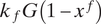 $ {k}_fG\left(1-{x}^f\right) $
and applying the equilibrium condition, we get the expression given in this claim. Note that the denominator has the same sign as
 $ \partial F\left({x}^f\left({y}_1\right);{y}_1\right)/\partial {x}^f $
, which is positive because
 $ F\left(\cdot; {y}_1\right) $
is single-crossing from below for
 $ {x}^f\in \left[0,{y}_1-\theta \right] $
. Moreover, since both
 $ \lambda \left(\cdot \right) $
and
 $ {c}_f $
are strictly positive, we have
 $ \partial {x}^f/\partial {y}_1>1/2 $
. A similar exercise gives
 $ \partial {x}^f/\partial \theta =-2\partial {x}^f/\partial {y}_1<-1 $
. □
Since
 $ A=1-{x}^f\left({y}_1;\theta \right) $
, the comparative statics for
 $ A $
have opposite signs to those for
 $ {x}^f $
. The second part of the proposition then follows immediately from Claim 1. ■
Proof of Proposition 1. Define
 $$ I\left({y}_1;\theta \right) := -\frac{\partial }{\partial {y}_1}\log G\left(1-{x}^f\left({y}_1;\theta \right)\right)=\lambda \left(1-{x}^f\left({y}_1;\theta \right)\right)\frac{\partial {x}^f\left({y}_1;\theta \right)}{\partial {y}_1}. $$
Claim 2. For
 $ {y}_1>{y}_{\mathrm{min}} $
,
 $ I\left({y}_1;\theta \right) $
is increasing in
 $ {y}_1 $
and decreasing in
 $ \theta $
. Moreover,
 $ I\left({y}_{\mathrm{min}};\theta \right)<\lambda \left(1-\left({y}_{\mathrm{min}}-\theta \right)\right) $
.
Proof. From Claim 1, we see that
 $ \partial {x}^f/\partial {y}_1 $
depends on
 $ {y}_1 $
only through
 $ {x}^f $
. Since
 $ \partial {x}^f/\partial {y}_1 $
increases in
 $ {x}^f $
, and
 $ {x}^f $
increases in
 $ {y}_1 $
,
 $ \partial {x}^f/\partial {y}_1 $
is increasing in
 $ {y}_1 $
. Moreover, log-concavity of
 $ G $
implies that
 $ \lambda \left(1-{x}^f\left({y}_1;\theta \right)\right) $
is increasing in
 $ {y}_1 $
. It then follows that
 $ I\left({y}_1;\theta \right) $
increases in
 $ {y}_1 $
. Similarly,
 $ I\left({y}_1;\theta \right) $
depends on
 $ \theta $
only through
 $ {x}^f $
. By Claim 1, we have
 $ \partial I/\partial \theta =-2\partial I/\partial {y}_1<0 $
. For the last part of this claim, it suffices to show that
 $ \partial {x}^f\left({y}_{\mathrm{min}}\left(\theta \right);\theta \right)/\partial {y}_1<1 $
. Recall that, in the proof of Lemma 1,
 $ \tilde{F}\left({y}_{\mathrm{min}}\right)=0 $
means that the marginal attacker corresponding to
 $ {y}_1={y}_{\mathrm{min}} $
is
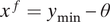 $ {x}^f={y}_{\mathrm{min}}-\theta $
. Using the expression for
 $ \partial {x}^f/\partial {y}_1 $
provided therein, we obtain
 $$ \frac{\partial {x}^f\left({y}_{\mathrm{min}}\left(\theta \right);\theta \right)}{\partial {y}_1}=\frac{1}{2-\lambda \left(1-\left({y}_{\mathrm{min}}-\theta \right)\right)\left({y}_{\mathrm{min}}-{y}_0\right)}. $$
But
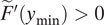 $ \tilde{F}\hbox{'}\left({y}_{\mathrm{min}}\right)>0 $
implies
 $ 1-\lambda \Big(1-\left({y}_{\mathrm{min}}-\theta, )\right)\left({y}_{\mathrm{min}}-{y}_0\right)>0 $
, and the claim follows. □
Since
 $ I\left({y}_1;\theta \right) $
increases in
 $ {y}_1 $
by Claim 2, the maximization problem (3) is quasiconcave for
 $ {y}_1\in \left[{y}_{\mathrm{min}},{x}^m+\theta \right] $
. Furthermore, Claim 2 implies that
 $$ 1-I\left({y}_{\mathrm{min}};\theta \right)\left({y}_{\mathrm{min}}-{y}_0\right)>1-\lambda \left(1-\left({y}_{\mathrm{min}}-\theta \right)\right)\left({y}_{\mathrm{min}}-{y}_0\right)>0. $$
This contradicts the necessary condition for the corner solution
 $ {y}_1={y}_{\mathrm{min}} $
to be optimal. The first-order condition for optimality therefore gives either an interior solution or a corner solution at
 $ {y}_1={x}^m+\theta $
. For the corner solution
 $ {y}_1^{\ast }={x}^m+\theta $
to be optimal, we require
 $$ 1-I\left({x}^m+\theta; \theta \right)\left({x}^m+\theta -{y}_0\right)\ge 0. $$
The left-hand-side of the above is strictly positive at
 $ {x}^m={y}_{\mathrm{min}}-\theta $
, and it is strictly decreasing in
 $ {x}^m $
. There exists a unique
 $ \hat{x}\left(\theta \right)>{y}_{\mathrm{min}}-\theta $
such that the left-hand-side is equal to
 $ 0 $
when
 $ {x}^m=\hat{x}\left(\theta \right) $
. When
 $ {x}^m>\hat{x}\left(\theta \right) $
,
 $ {y}_1^{\ast }=\hat{x}\left(\theta \right)+\theta $
satisfies the first-order condition for an interior solution.
At an interior solution, we have
 $$ 1-I\left(\hat{x}\left(\theta \right)+\theta; \theta \right)\left(\hat{x}\left(\theta \right)+\theta -{y}_0\right)=0. $$
Differentiate the above equation to get
 $ \partial \hat{x}\left(\theta \right)/\partial \theta \in \left(-1,1\right) $
. Since
 $ {y}_1^{\ast }=\min \left\{{x}^m,\hat{x}\left(\theta \right)\right\}+\theta $
, we have
 $ \partial {y}_1^{\ast }/\partial \theta \in \left(0,2\right) $
. Moreover,
 $ \partial {y}_1^{\ast }/\partial \theta <2 $
and Claim 1 together imply that
 $ {x}^f\left({y}_1^{\ast}\left({x}^m;\theta \right);\theta \right) $
decreases in
 $ \theta $
. It follows that
 $ G\left(1-{x}^f\left({y}_1^{\ast}\left({x}^m;\theta \right);\theta \right)\right) $
increases in
 $ \theta $
. ■
Proof of Lemma 2. For
 $ {x}^m\ge {y}_{\mathrm{min}}\left({\theta}_L\right)-{\theta}_L $
, let the difference in payoff between choosing
 $ {y}_1^{H\ast } $
and
 $ {y}_1^{L\ast } $
in state
 $ {\theta}_L $
be represented by
 $$ {\tilde{\Delta}}_L({x}^m) := {G}^{L\ast }(u\left({y}_1^{L\ast },{\theta}_L,{x}^m\right)-u\Big({y}_0,{\theta}_L,{x}^m\Big))-{G}^{H\ast}\left(u\left({y}_1^{H\ast },{\theta}_L,{x}^m\right)-u\Big({y}_0,{\theta}_L,{x}^m\Big)\right), $$
where
 $ {y}_1^{H\ast } $
and
 $ {y}_1^{L\ast } $
depend on
 $ {x}^m $
. We show that
 $ {\tilde{\Delta}}_L\left({x}^m\right) $
decreases in
 $ {x}^m $
. There are four cases to consider:
(a) If
 $ {x}^m\le \min \left\{\hat{x}\left({\theta}_H\right),\hat{x}\left({\theta}_L\right)\right\} $
, then
 $ {y}_1^{H\ast }={x}^m+{\theta}_H $
and
 $ {y}_1^{L\ast }={x}^m+{\theta}_L $
. This gives
 $$ {\tilde{\Delta}}_L\left({x}^m\right)={G}^{L\ast}\left({x}^m+{\theta}_L-{y}_0\right)-{G}^{H\ast}\left(2{x}^m+2{\theta}_L-\left({x}^m+{\theta}_H\right)-{y}_0\right). $$
The derivative with respect to
 $ {x}^m $
is
 $$ \tilde{\Delta}{\hbox{'}}_L\left({x}^m\right)=\left[{G}^{L\ast}\left(1-{I}^{L\ast}\left({x}^m+{\theta}_L-{y}_0\right)\right)-{G}^{H\ast}\left(1-{I}^{H\ast}\left({x}^m+{\theta}_L-{y}_0\right)\right)\right]-{G}^{H\ast }{I}^{H\ast}\left({\theta}_H-{\theta}_L\right), $$
where
 $ {I}^{H\ast} := I\left({y}_1^{H\ast };{\theta}_H\right) $
and
 $ {I}^{L\ast} := I\left({y}_1^{L\ast };{\theta}_L\right) $
. The term in brackets is negative because
 $ {G}^{L\ast }<{G}^{H\ast } $
(Proposition 1) and
 $ {I}^{L\ast }>{I}^{H\ast } $
(which follows from Claim 1 and the fact that
 $ I $
depends on
 $ {y}_1 $
and
 $ \theta $
only through
 $ {x}^f\left({y}_1;\theta \right) $
). We therefore have
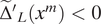 $ \tilde{\Delta}{\hbox{'}}_L\left({x}^m\right)<0 $
.
(b) If
 $ {x}^m\in \left[\min \left\{\hat{x}\left({\theta}_H\right),\hat{x}\left({\theta}_L\right)\right\},\max \left\{\hat{x}\left({\theta}_H\right),\hat{x}\left({\theta}_L\right)\right\}\right] $
, then
 $ {y}_1^{H\ast }=\min \left\{{x}^m,\hat{x}\left({\theta}_H\right)\right\}+{\theta}_H $
and
 $ {y}_1^{L\ast }=\min \left\{{x}^m,\hat{x}\left({\theta}_L\right)\right\}+{\theta}_L $
. This gives
 $$ {\tilde{\Delta}}_L\left({x}^m\right)={G}^{L\ast}\left(\min \Big\{{x}^m,\hat{x}\left({\theta}_L\right)\Big\}+{\theta}_L-{y}_0\right)-{G}^{H\ast}\left(2{x}^m+2{\theta}_L-\left(\min \right\{{x}^m,\hat{x}\left({\theta}_H\right)\left\}+{\theta}_H\right)-{y}_0\right). $$
Therefore,
 $$ {\tilde{\Delta}}_L^{\prime}\left({x}^m\right)=\left\{\begin{array}{cc}{G}^{L\ast}\left(1-{I}^{L\ast}\left({x}^m+{\theta}_L-{y}_0\right)\right)-2{G}^{H\ast} & \mathrm{if} \hat{x}\left({\theta}_H\right)<\hat{x}\left({\theta}_L\right),\\ {}-{G}^{H\ast}\left(1-{I}^{H\ast}\left({x}^m+{\theta}_L-{y}_0\right)+{I}^{H\ast}\left({\theta}_H-{\theta}_L\right)\right)& \mathrm{if} \hat{x}\left({\theta}_H\right)>\hat{x}\left({\theta}_L\right).\end{array}\right. $$
In either case, we have
 $ {\tilde{\Delta}}_L^{\prime}\left({x}^m\right)<0 $
.
(c) If
 $ {x}^m\in \left(\max \left\{\hat{x}\left({\theta}_H\right),\hat{x}\left({\theta}_L\right)\right\},\hat{x}\left({\theta}_H\right)+{\theta}_H-{\theta}_L\right) $
, then
 $ {y}_1^{H\ast }=\hat{x}\left({\theta}_H\right)+{\theta}_H $
and
 $ {y}_1^{L\ast }=\hat{x}\left({\theta}_L\right)+{\theta}_L $
. This gives
 $$ {\tilde{\Delta}}_L\left({x}^m\right)={G}^{L\ast}\left(\hat{x}\left({\theta}_L\right)+{\theta}_L-{y}_0\right)-{G}^{H\ast}\left(2{x}^m+2{\theta}_L-\left(\hat{x}\left({\theta}_H\right)+{\theta}_H\right)-{y}_0\right), $$
with
 $ {\tilde{\Delta}}_L^{\prime}\left({x}^m\right)=-2{G}^{H\ast }<0 $
.
(d) If
 $ {x}^m\ge \hat{x}\left({\theta}_H\right)+{\theta}_H-{\theta}_L $
, then
 $ {y}_1^{H\ast }=\hat{x}\left({\theta}_H\right)+{\theta}_H $
,
 $ {y}_1^{L\ast }=\hat{x}\left({\theta}_L\right)+{\theta}_L $
, and
 $$ {\tilde{\Delta}}_L\left({x}^m\right)={G}^{L\ast}\left(\hat{x}\left({\theta}_L\right)+{\theta}_L-{y}_0\right)-{G}^{H\ast}\left(\hat{x}\left({\theta}_H\right)+{\theta}_H-{y}_0\right)<0. $$
In this case,
 $ {\tilde{\Delta}}_L\left({x}^m\right) $
is constant with respect to
 $ {x}^m $
.
Because
 $ {\tilde{\Delta}}_L\left({x}^m\right) $
is continuous in
 $ {x}^m $
, these four cases show that it is decreasing in
 $ {x}^m $
for all
 $ {x}^m\ge {y}_{\mathrm{min}}\left({\theta}_L\right)-{\theta}_L $
. Moreover,
 $$ {\displaystyle \begin{array}{l}{\tilde{\Delta}}_L\left(\hat{x}\left({\theta}_H\right)\right)={G}^{H\ast}\left({y}_1^{L\ast }-\hat{x}\left({\theta}_H\right)-2{\theta}_L+{\theta}_H\right)+\left({G}^{L\ast }-{G}^{H\ast}\right)\left({y}_1^{L\ast }-{y}_0\right)\\ {}>{G}^{H\ast}\left({y}_1^{L\ast }-\hat{x}\left({\theta}_H\right)-2{\theta}_L+{\theta}_H+\left(\log {G}^{L\ast }-\log {G}^{H\ast}\right)\left({y}_1^{L\ast }-{y}_0\right)\right),\end{array}} $$
where the inequality follows from the fact that
 $ t-1>\log t $
for any positive
 $ t $
. Now,
 $$ {\displaystyle \begin{array}{l}\log {G}^{L\ast }-\log {G}^{H\ast }=\log G\left(1-{x}^f\left({y}_1^{L\ast };{\theta}_L\right)\right)-\log G\left(1-{x}^f\left({y}_1^{H\ast }-2\left({\theta}_H-{\theta}_L\right);{\theta}_L\right)\right)\\ {}=-{\int}_{y_1^{H\ast }-2\left({\theta}_H-{\theta}_L\right)}^{y_1^{L\ast }}I\left({y}_1;{\theta}_L\right) \mathrm{d}{y}_1\\ {}>-{I}^{L\ast}\left({y}_1^{L\ast }-\hat{x}\left({\theta}_H\right)-2{\theta}_L+{\theta}_H\right),\end{array}} $$
where the first equality follows from Claim 1 and the inequality follows from Claim 2. This gives
 $$ {\tilde{\Delta}}_L\left(\hat{x}\left({\theta}_H\right)\right)>{G}^{H\ast}\left({y}_1^{L\ast }-\hat{x}\left({\theta}_H\right)-2{\theta}_L+{\theta}_H\right)\left(1-{I}^{L\ast}\left({y}_1^{L\ast }-{y}_0\right)\right)\ge 0, $$
where the last inequality follows from the first-order condition (4). In part (d) above, we have also shown that
 $ {\tilde{\Delta}}_L\left(\hat{x}\left({\theta}_H\right)+{\theta}_H-{\theta}_L\right)<0 $
. Thus, there exists a unique
 $ {x}^{\dagger}\in \left(\hat{x}\left({\theta}_H\right),\hat{x}\left({\theta}_H\right)+{\theta}_H-{\theta}_L\right) $
such that
 $ {\tilde{\Delta}}_L\left({x}^m\right)\ge 0 $
if
 $ {x}^m\le {x}^{\dagger } $
and
 $ {\tilde{\Delta}}_L\left({x}^m\right)<0 $
if
 $ {x}^m>{x}^{\dagger } $
.
For
 $ {x}^m\le {x}^{\dagger } $
, the leader prefers choosing
 $ {y}_1^{L\ast } $
to choosing
 $ {y}_1^{H\ast } $
in state
 $ {\theta}_L $
because
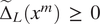 $ {\tilde{\Delta}}_L\left({x}^m\right) \ge 0 $
. In state
 $ {\theta}_H $
, the leader prefers choosing
 $ {y}_1^{H\ast } $
to choosing
 $ {y}_1^{L\ast } $
because the former is closer to the leader’s ideal policy (
 $ {x}^m+{\theta}_H\ge {y}_1^{H\ast }>{y}_1^{L\ast } $
) and because the probability of success is higher (
 $ {G}^{H\ast }>{G}^{L\ast } $
). Given such choices, citizens correctly infer the state based on the agenda chosen by the leader, and therefore the full-information outcome constitutes an equilibrium outcome.
For
 $ {x}^m>{x}^{\dagger } $
, the full-information outcome cannot be supported in equilibrium because
 $ {\tilde{\Delta}}_L\left({x}^m\right)<0 $
implies that the leader would deviate to choosing
 $ {y}_1^{H\ast } $
in state
 $ {\theta}_L $
. ■
Proof of Proposition 2.
Part (i). Suppose
 $ {\hat{y}}_1^L\ne {y}_1^{L\ast } $
. If
 $ {x}^m $
deviates to
 $ {y}_1^{L\ast } $
, the worst inference that citizens can make is that the state is low, which is the same as the equilibrium inference. But by construction,
 $ {y}_1^{L\ast } $
is preferred to
 $ {\hat{y}}_1^L $
, a contradiction.
Part (ii). In any separating equilibrium, the policy
 $ {y}_1^H $
chosen in the high state has to satisfy the incentive constraint for the leader in the low state:
 $$ {\displaystyle \begin{array}{l}{\Delta}_L\left({x}^m;{y}_1^H\right)=G(1-{x}^f({\hat{y}}_1^L;{\theta}_L))(u({\hat{y}}_1^L,{\theta}_L,{x}^m)-u\Big({y}_0,{\theta}_L,{x}^m\Big))\\ {}-G(1-{x}^f({y}_1^H;{\theta}_H))\left(u\left({y}_1^H,{\theta}_L,{x}^m\right)-u\Big({y}_0,{\theta}_L,{x}^m\Big)\right)\ge 0,\end{array}} $$
where
 $ {\hat{y}}_1^L={y}_1^{L\ast } $
depends on
 $ {x}^m $
. For
 $ {x}^m>{x}^{\dagger } $
, Lemma 2 establishes that
 $ {\Delta}_L\left({x}^m;{y}_1^{H\ast}\right)={\tilde{\Delta}}_L\left({x}^m\right)<0 $
. There are three cases.
(a) If
 $ {y}_1^{H\ast }>{x}^m+{\theta}_L $
, then for any
 $ {y}_1^H\in \left({x}^m+{\theta}_L,{y}_1^{H^{\ast }}\right) $
,
 $ {\Delta}_L\left({x}^m;\cdot \right) $
is strictly increasing, implying that
 $ {\Delta}_L\left({x}^m;{y}_1^H\right)<{\Delta}_L\left({x}^m;{y}_1^{H\ast}\right)<0 $
for such
 $ {y}_1^H $
.
(b) For any
 $ {y}_1^H\in \left[{\hat{y}}_1^L,\min \left\{{y}_1^{H\ast },{x}^m+{\theta}_L\right\}\right] $
,
 $ {\Delta}_L\left({x}^m;\cdot \right) $
is strictly decreasing. Therefore,
 $ {\Delta}_L\left({x}^m;{y}_1^H\right)<{\Delta}_L\left({x}^m;{\hat{y}}_1^L\right)<0 $
.
(c) For
 $ {y}_1^H<{\hat{y}}_1^L $
,
 $ {\Delta}_L\left({x}^m;\cdot \right) $
is strictly decreasing. There exists
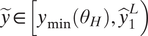 $ \tilde{y}\in \left[{y}_{\mathrm{min}}\left({\theta}_H\right),{\hat{y}}_1^L\right) $
such that
 $ {\Delta}_L\left({x}^m;{y}_1^H\right)<0 $
for all
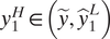 $ {y}_1^H\in \left(\tilde{y},{\hat{y}}_1^L\right) $
. Such
 $ {y}_1^H $
cannot be part of a separating equilibrium because it violates the incentive constraint in the low state. For
 $ {y}_1^H<\tilde{y} $
, we have
 $ {\Delta}_L\left({x}^m;{y}_1^H\right)>0 $
. But because the reward from success weakly increases in the state, this implies
 $$ {\displaystyle \begin{array}{l}{\Delta}_H\left({x}^m;{y}_1^H\right) := G\left(1-{x}^f\left({y}_1^H;{\theta}_H\right)\right)\left(u\left({y}_1^H,{\theta}_H,{x}^m\right)-u\Big({y}_0,{\theta}_H,{x}^m\Big)\right)\\ {}-G(1-{x}^f({\hat{y}}_1^L;{\theta}_L))(u({\hat{y}}_1^L,{\theta}_H,{x}^m)-u\Big({y}_0,{\theta}_H,{x}^m\Big))<0,\end{array}} $$
which violates the incentive constraint in the high state. If
 $ {y}_1^H=\tilde{y} $
, it is possible to have a knife-edge equilibrium in which the leader chooses
 $ {\hat{y}}_1^L $
in the low state and chooses
 $ \tilde{y}<{\hat{y}}_1^L $
in the high state, and the incentive constraints in both states are satisfied with equality. However, such a knife-edge equilibrium does not satisfy the D1 refinement. Consider a deviation to some
 $ {y}^{\prime}\in \left({x}^m+{\theta}_L,{x}^m+{\theta}_H\right] $
. For any given belief, the high type gains more from such deviation than does the low type. According to the D1 criterion, citizens should assign off-equilibrium belief that such deviation comes from the high type. Given such off-equilibrium belief, the high type indeed could profitably deviate from
 $ \tilde{y} $
to
 $ {y}^{\prime } $
, which means that the knife-edge case does not satisfy the D1 equilibrium refinement.
We conclude that any separating equilibrium that satisfies the D1 refinement must satisfy
 $ {\hat{y}}_1^H>{y}_1^{H\ast } $
. Because
 $ {\Delta}_L\left({x}^m;{y}_1^H\right) $
is strictly increasing for
 $ {y}_1^H>{y}_1^{H\ast } $
and is positive when
 $ {y}_1^H $
is sufficiently large, there exists a unique
 $ {\hat{y}}_1^H>{y}_1^{H\ast } $
that satisfies
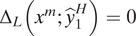 $ {\Delta}_L\left({x}^m;{\hat{y}}_1^H\right)=0 $
. The pair
 $ \left({\hat{y}}_1^L,{\hat{y}}_1^H\right) $
constitute a separating equilibrium because the leader weakly prefers
 $ {\hat{y}}_1^L $
to
 $ {\hat{y}}_1^H $
in the low state. Moreover, because
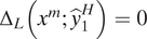 $ {\Delta}_L\left({x}^m;{\hat{y}}_1^H\right)=0 $
implies
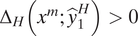 $ {\Delta}_H\left({x}^m;{\hat{y}}_1^H\right)>0 $
, the leader strictly prefers
 $ {\hat{y}}_1^H $
to
 $ {\hat{y}}_1^L $
in the high state. This equilibrium can be supported by off-equilibrium beliefs which assign probability
 $ 1 $
that the state is high when the policy
 $ {y}_1\ge {\hat{y}}_1^H $
and probability
 $ 0 $
otherwise.
To show that these beliefs satisfy the D1 criterion, we need the following result.
Claim 3. For any
 $ {x}^m\ge {x}^{\dagger } $
,
 $ {\hat{y}}_1^H\left({x}^m\right)\in \left({x}^m+{\theta}_L,{x}^m+{\theta}_H\right) $
.
Proof. Let
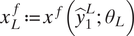 $ {x}_L^f := {x}^f\left({\hat{y}}_1^L;{\theta}_L\right) $
and
 $ {x}_H^f := {x}^f\left({x}^m+{\theta}_H;{\theta}_H\right)={x}^f\left({x}^m+2{\theta}_L-{\theta}_H;{\theta}_L\right) $
. By Claim 1, we see that
 $ {x}_L^f\ge {x}_H^f $
(and
 $ {G}^L\le {G}^H $
) if and only if
 $ {\hat{y}}_1^L\ge {x}^m+2{\theta}_L-{\theta}_H $
. We have
 $$ {\displaystyle \begin{array}{c}{\Delta}_L\left({x}^m;{x}^m+{\theta}_H\right)={G}^H\left({\hat{y}}_1^L-{x}^m-2{\theta}_L+{\theta}_H\right)+\left({G}^L-{G}^H\right)\left({\hat{y}}_1^L-{y}_0\right)>{G}^H\left({\hat{y}}_1^L-{x}^m-2{\theta}_L+{\theta}_H+\left(\log {G}^L-\log {G}^H\right)\left({\hat{y}}_1^L-{y}_0\right)\right)>{G}^H\left({\hat{y}}_1^L-{x}^m-2{\theta}_L+{\theta}_H+{I}^L\left({x}^m+2{\theta}_L-{\theta}_H-{\hat{y}}_1^L\right)\left({\hat{y}}_1^L-{y}_0\right)\right)={G}^H\left({\hat{y}}_1^L-{x}^m-2{\theta}_L+{\theta}_H\right)\left(1-{I}^L\left({\hat{y}}_1^L-{y}_0\right)\right),\end{array}} $$
where
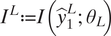 $ {I}^L:= I\left({\hat{y}}_1^L;{\theta}_L\right) $
. If
 $ {x}^m<\hat{x}\left({\theta}_L\right) $
,
 $ {\hat{y}}_1^L-{x}^m-2{\theta}_L+{\theta}_H>0 $
and
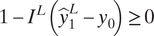 $ 1-{I}^L\left({\hat{y}}_1^L-{y}_0\right)\ge 0 $
. If
 $ {x}^m\ge \hat{x}\left({\theta}_L\right) $
,
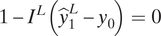 $ 1-{I}^L\left({\hat{y}}_1^L-{y}_0\right)=0 $
. In either case,
 $ {\Delta}_L\left({x}^m;{x}^m+{\theta}_H\right)>0 $
.
Now, we let
 $ {x}_H^f $
,
 $ {G}^H $
, and
 $ {I}^H $
represent the values of the relevant variables at the point
 $ {y}_1^H={x}^m+{\theta}_L $
. We have
 $$ {\displaystyle \begin{array}{c}{\Delta}_L\left({x}^m;{x}^m+{\theta}_L\right)={G}^L\left({\hat{y}}_1^L-{x}^m-{\theta}_L\right)-\left({G}^H-{G}^L\right)\left({x}^m+{\theta}_L-{y}_0\right)<{G}^L\left({\hat{y}}_1^L-{x}^m-{\theta}_L+\left(\log {G}^L-\log {G}^H\right)\left({x}^m+{\theta}_L-{y}_0\right)\right).\end{array}} $$
If
 $ {\hat{y}}_1^L\in \left[{x}^m+{\theta}_L-2\left({\theta}_H-{\theta}_L\right),{x}^m+{\theta}_L\right] $
, then
 $ {G}^L\le {G}^H $
, and therefore the above expression is negative. If
 $ {\hat{y}}_1^L<{x}^m+{\theta}_L-2\left({\theta}_H-{\theta}_L\right) $
, then
 $ {G}^L>{G}^H $
, and we have
 $$ {\displaystyle \begin{array}{l}{\Delta}_L\left({x}^m;{x}^m+{\theta}_L\right)<{G}^L\left({\hat{y}}_1^L-{x}^m-{\theta}_L+{I}^H\left({x}^m+{\theta}_L-2\left({\theta}_H-{\theta}_L\right)-{\hat{y}}_1^L\right)\left({x}^m+{\theta}_L-{y}_0\right)\right)\\ {}<-{G}^H\left({\theta}_H-{\theta}_L\right),\end{array}}, $$
where the second inequality follows because
 $ {x}^m>{x}^{\dagger }>\hat{x}\left({\theta}_H\right) $
implies that
 $ {I}^H\left({x}^m+{\theta}_L-{y}_0\right)<1 $
. We conclude that
 $ {\Delta}_L\left({x}^m;{x}^m+{\theta}_L\right)<0 $
.
Since
 $ {\Delta}_L\left({x}^m;{x}^m+{\theta}_H\right)>0>{\Delta}_L\left({x}^m;{x}^m+{\theta}_L\right) $
, and
 $ {\Delta}_L\left({x}^m;\cdot \right) $
is strictly increasing in the relevant range, the
 $ {\hat{y}}_1^H $
that satisfies the binding incentive constraint
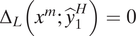 $ {\Delta}_L\left({x}^m;{\hat{y}}_1^H\right)=0 $
is unique and satisfies
 $ {\hat{y}}_1^H\in \left({x}^m+{\theta}_L,{x}^m+{\theta}_H\right) $
. □
Consider an off-equilibrium policy
 $ {y}^{\prime}\in \left[{x}^m+{\theta}_L,{x}^m+{\theta}_H\right] $
. The minimum success probability
 $ {G}^{\prime } $
that would induce the high type to deviate to
 $ {y}^{\prime } $
requires
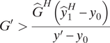 $$ {G}^{\prime }>\frac{{\hat{G}}^H\left({\hat{y}}_1^H-{y}_0\right)}{y^{\prime }-{y}_0} $$
and the minimum
 $ {G}^{\prime } $
needed to induce the low type to deviate requires
 $$ {G}^{\prime }>\frac{{\hat{G}}^L\left({\hat{y}}_1^L-{y}_0\right)}{2{x}^m+2{\theta}_L-{y}^{\prime }-{y}_0}. $$
Using the binding incentive constraint (6), the set of beliefs that would support deviation by the high type strictly contains the set of beliefs that would support deviation by the low type if and only if
 $$ \frac{2{x}^m+2{\theta}_L-{\hat{y}}_1^H-{y}_0}{{\hat{y}}_1^H-{y}_0}>\frac{2{x}^m+2{\theta}_L-{y}^{\prime }-{y}_0}{y^{\prime }-{y}_0}, $$
which is true if and only if
 $ {y}^{\prime }>{\hat{y}}_1^H $
. Thus the D1 criterion requires assigning probability
 $ 1 $
that the state is high if
 $ {y}^{\prime }>{\hat{y}}_1^H $
and probability
 $ 0 $
if
 $ {y}^{\prime }<{\hat{y}}_1^H $
.
For deviations
 $ {y}^{\prime }<{x}^m+{\theta}_L $
, the corresponding comparison requires
 $$ {\hat{G}}^L\left({\hat{y}}_1^L-{y}_0\right)>{\hat{G}}^H\left({\hat{y}}_1^H-{y}_0\right), $$
which contradicts the binding incentive constraint (6). Therefore, citizens assign probability
 $ 0 $
that the state is high upon observing such an agenda. For
 $ {y}^{\prime }>{x}^m+{\theta}_H $
, the comparison requires
 $$ \frac{2{x}^m+2{\theta}_L-{\hat{y}}_1^H-{y}_0}{{\hat{y}}_1^H-{y}_0}>\frac{2{x}^m+2{\theta}_L-{y}^{\prime }-{y}_0}{2{x}^m+2{\theta}_H-{y}^{\prime }-{y}_0}, $$
which is always true. In this case, the off-equilibrium belief that the state is high with probability
 $ 1 $
is again consistent with the D1 criterion.
Part (iii). Use implicit differentiation of
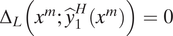 $ {\Delta}_L\left({x}^m;{\hat{y}}_1^H\left({x}^m\right)\right)=0 $
to get
 $$ \frac{\partial {\hat{y}}_1^H}{\partial {x}^m}=\left\{\begin{array}{cc}\frac{2{\hat{G}}^H-{\hat{G}}^L\left(1-{I}^L\left({x}^m+{\theta}_L-{y}_0\right)\right)}{{\hat{G}}^H\left(1+{I}^H\left(2{x}^m+2{\theta}_L-{\hat{y}}_1^H-{y}_0\right)\right)}& \mathrm{if}\;{x}^m<\hat{x}\left({\theta}_L\right),\\ {}\frac{2}{1+{I}^H\left(2{x}^m+2{\theta}_L-{\hat{y}}_1^H-{y}_0\right)} & \mathrm{if}\;{x}^m>\hat{x}\left({\theta}_L\right).\end{array}\right. $$
By Lemma 2,
 $ {x}^m<\hat{x}\left({\theta}_L\right) $
implies
 $ {\hat{G}}^H>{\hat{G}}^L $
. Therefore,
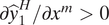 $ \partial {\hat{y}}_1^H/\partial {x}^m>0 $
. For comparative statics with respect to
 $ {\theta}_H $
, we have
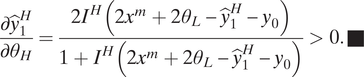 $$ \frac{\partial {\hat{y}}_1^H}{\partial {\theta}_H}=\frac{2{I}^H\left(2{x}^m+2{\theta}_L-{\hat{y}}_1^H-{y}_0\right)}{1+{I}^H\left(2{x}^m+2{\theta}_L-{\hat{y}}_1^H-{y}_0\right)}>0.\blacksquare $$
Proof of Proposition 3. Two conditions are sufficient for this proposition:
 $ {y}_{\mathrm{min}}\left({\theta}_L\right)-{\theta}_L<1/2 $
and
 $ \min \left\{\hat{L}P\left(1/2;1/2\right),\hat{L}P\left(1;1\right)\right\}>0 $
. We first establish the following result.
Claim 4.
 $ \min \left\{\hat{L}P\left(1/2;1/2\right),\hat{L}P\left(1;1\right)\right\}>0 $
implies
 $ \hat{L}P\left({x}^m;{x}^m\right)>0 $
for all
 $ {x}^m\in \left[1/2,1\right] $
.
Proof. Consider the leader’s premium in the low state. We have
 $$ \frac{\mathrm{d}}{\mathrm{d}{x}^m} LP\left({x}^m;{\hat{y}}_1^L\left({x}^m\right),{\theta}_L\right)=\left\{\begin{array}{cc}{k}_l{\hat{G}}^L\left(1-{I}^L\left({x}^m+{\theta}_L-{y}_0\right)\right)& \mathrm{if}\;{x}^m<\hat{x}\left({\theta}_L\right),\\ {}0& \mathrm{if}\;{x}^m>\hat{x}\left({\theta}_L\right).\end{array}\right. $$
This shows that
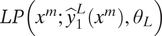 $ LP\left({x}^m;{\hat{y}}_1^L\left({x}^m\right),{\theta}_L\right) $
is increasing for
 $ {x}^m<\hat{x}\left({\theta}_L\right) $
and is constant for
 $ {x}^m>\hat{x}\left({\theta}_L\right) $
. In the high state,
 $$ \frac{\mathrm{d}}{\mathrm{d}{x}^m} LP\left({x}^m;{\hat{y}}_1^H\left({x}^m\right),{\theta}_H\right)={k}_l{\hat{G}}^H\left(1-{I}^H\left({\hat{y}}_1^H-{y}_0\right)\right)\frac{\partial {\hat{y}}_1^H}{\partial {x}^m}. $$
If
 $ {x}^m>{x}^{\dagger } $
,
 $ {I}^H\left({\hat{y}}_1^H-{y}_0\right)>{I}^H\left({y}_1^{H\ast }-{y}_0\right)>1 $
. Therefore,
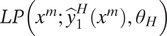 $ LP\left({x}^m;{\hat{y}}_1^H\left({x}^m\right),{\theta}_H\right) $
is increasing for
 $ {x}^m<\hat{x}\left({\theta}_H\right) $
, constant for
 $ {x}^m\in \left(\hat{x}\left({\theta}_H\right),{x}^{\dagger}\right) $
, and decreasing for
 $ {x}^m>{x}^{\dagger } $
. Because
 $ \hat{L}P\left({x}^m;{x}^m\right) $
is a weighted average of the leader’s premium in the two states, its minimum on the interval
 $ \left[1/2,1\right] $
must be at either corner of the interval. □
Claim 4 implies that the mapping
 $ M $
is well-defined on
 $ \left[1/2,1\right] $
. It is continuous because
 $ {x}^m\ge 1/2 $
implies that
 $ {x}^m\ge 1/2>{y}_{\mathrm{min}}\left({\theta}_L\right)-{\theta}_L $
. Moreover,
 $ {x}^l\left(1/2\right)>0 $
implies
 $ M\left(1/2\right)>1/2 $
and
 $ {x}^l(1)<1 $
implies
 $ M(1)<1 $
. Thus a fixed point of the the mapping
 $ M $
exists.
We next show that
 $ {M}^{\prime}\left({x}^m\right)>0 $
. Note that Claim 2 implies that
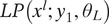 $ LP\left({x}^l;{y}_1,{\theta}_L\right) $
is quasiconcave in
 $ {y}_1 $
, and it is strictly decreasing in
 $ {y}_1 $
for all
 $ {y}_1>{y}_1^{\ast}\left({x}^l;{\theta}_L\right) $
. Therefore,
 $ {\hat{y}}_1^L={y}_1^{\ast}\left({x}^m;{\theta}_L\right)\ge {y}_1^{\ast}\left({x}^l;{\theta}_L\right) $
implies that
 $$ \frac{\partial {LP}^L}{\partial {x}^m}=\frac{\partial LP\left({x}^l;{\hat{y}}_1^L,{\theta}_H\right)}{\partial {y}_1}\frac{\partial {\hat{y}}_1^L\left({x}^m\right)}{\partial {x}^m}\le 0, $$
with equality if only if
 $ {x}^m>\hat{x}\left({\theta}_L\right) $
. Similarly,
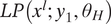 $ LP\left({x}^l;{y}_1,{\theta}_H\right) $
is strictly decreasing in
 $ {y}_1 $
for all
 $ {y}_1>{y}_1^{\ast}\left({x}^l;{\theta}_H\right) $
. Therefore,
 $ {\hat{y}}_1^H\ge {y}_1^{\ast}\left({x}^m;{\theta}_H\right)\ge {y}_1^{\ast}\left({x}^l;{\theta}_H\right) $
implies that
 $ \partial {LP}^H/\partial {x}^m\le 0 $
, with equality if and only if
 $ {x}^m\in \left(\hat{x}\left({\theta}_H\right),{x}^{\dagger}\right) $
. Since both
 $ {LP}^L $
and
 $ {LP}^H $
decrease in
 $ {x}^m $
, a higher
 $ {x}^m $
lowers the expected leader’s premium
 $ \hat{L}P\left({x}_i;{x}^m\right) $
for every citizen
 $ i $
, and therefore raises
 $ {x}^l\left({x}^m\right) $
. This implies that
 $ M\left({x}^m\right) $
also becomes higher.
Claim 5. If
 $ {\theta}_H-{\theta}_L<1/3 $
, then
 $ {M}^{\prime}\left({x}_{\ast}^m\right)<1 $
.
Proof. For
 $ j\in \left\{H,L\right\} $
, let
 $ {LP}^j= LP\left({x}^l;{\hat{y}}_1^j\left({x}^m\right),{\theta}_j\right) $
. We have
 $$ \frac{\partial {LP}^L}{\partial {x}^m}+2\frac{\partial {LP}^L}{\partial {x}^l}=\left\{\begin{array}{ll}{k}_l{\hat{G}}^L\left[3-{I}^L\left(2{x}^l+2{\theta}_L-\left({x}^m+{\theta}_L\right)-{y}_0\right)\right]& \mathrm{if} {x}^m<\hat{x}\left({\theta}_L\right),\\ {}2{k}_l{\hat{G}}^L& \mathrm{if} {x}^m>\hat{x}\left({\theta}_L\right)>{x}^l,\\ {}0& \mathrm{if} {x}^l>\hat{x}\left({\theta}_L\right).\end{array}\right. $$
Because
 $ {x}^l<{x}^m $
, the bracketed term for the first case is greater than
 $ 3-{I}^L\left({x}^m+{\theta}_L-{y}_0\right) $
, which is positive by the first-order condition (4).
Furthermore, we have
 $$ \frac{\partial {LP}^H}{\partial {x}^m}+2\frac{\partial {LP}^H}{\partial {x}^l}={k}_l{\hat{G}}^H\left[4-\left(1+{I}^H\left(2{x}^l+2{\theta}_H-{\hat{y}}_1^H-{y}_0\right)\right)\frac{\partial {\hat{y}}_1^H}{\partial {x}^m}\right]. $$
From the proof of Proposition 2 (i.e., part [iii]), we see that the bracketed term is greater than or equal to
 $$ 4-2\frac{1+{I}^H\left(2{x}^l+2{\theta}_H - {\hat{y}}_1^H-{y}_0\right)}{1+{I}^H\left(2{x}^m+2{\theta}_L - {\hat{y}}_1^H-{y}_0\right)}. $$
A sufficient condition for the above expression to be positive when evaluated at the fixed points
 $ {x}^m={x}_{\ast}^m $
and
 $ {x}^l={x}^l\left({x}_{\ast}^m\right)=2{x}_{\ast}^m-1 $
is that
 $$ \frac{2{x}^l\left({x}_{\ast}^m\right)+2{\theta}_H-{\hat{y}}_{1\ast}^H-{y}_0}{2{x}_{\ast}^m+2{\theta}_L-{\hat{y}}_{1\ast}^H-{y}_0}\le 2. $$
The above inequality is true if and only if
 $$ \left[1-3\left({\theta}_H-{\theta}_L\right)\right]+\left({x}_{\ast}^m+{\theta}_H-{\hat{y}}_{1\ast}^H\right)+\left({x}_{\ast}^m-{x}^l\left({x}_{\ast}^m\right)\right)+\left({\theta}_L-{y}_0\right)\ge 0. $$
By Claim 3, the second bracketed term is positive. Therefore,
 $ {\theta}_H-{\theta}_L\le 1/3 $
implies that the inequality is true.
We have shown that for
 $ j\in \left\{H,L\right\} $
,
 $$ \sum \limits_{j=H,L}{\pi}_j\left(\frac{\partial {LP}^j}{\partial {x}^m}+2\frac{\partial {LP}^j}{\partial {x}^l}\right)>0 $$
when evaluated at
 $ \left({x}^m,{x}^l\right)=\left({x}_{\ast}^m,{x}_{\ast}^l\right) $
. By the implicit function theorem, this implies that
 $ \partial {x}^l\left({x}_{\ast}^m\right)/\partial {x}^m<2 $
, and hence
 $ {M}^{\prime}\left({x}_{\ast}^m\right)<1 $
. □
Claim 5 implies that
 $ M\left({x}^m\right)-{x}^m $
is single-crossing from above when
 $ {\theta}_H-{\theta}_L\le 1/3 $
. This shows that the fixed point
 $ {x}_{\ast}^m $
is unique. ■



















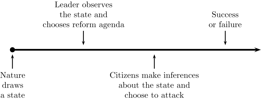
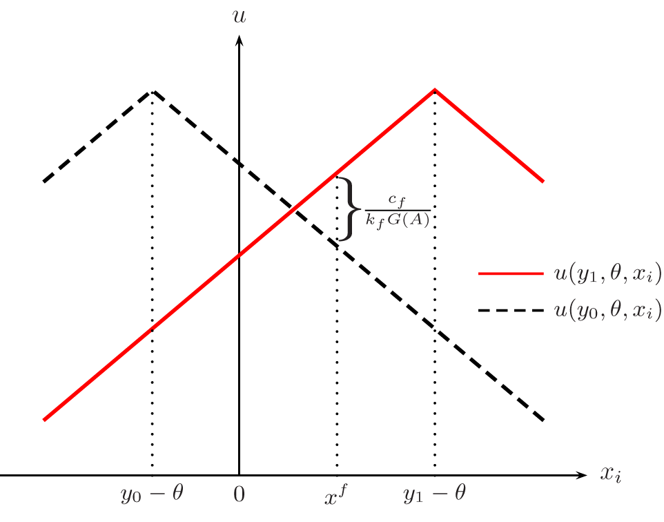


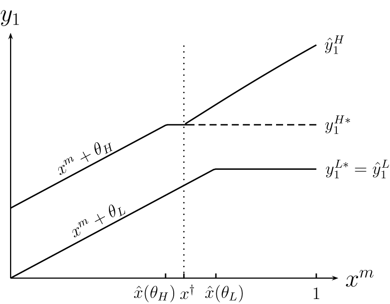


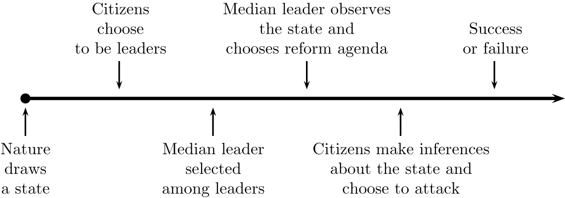
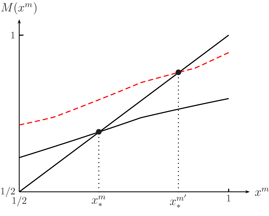


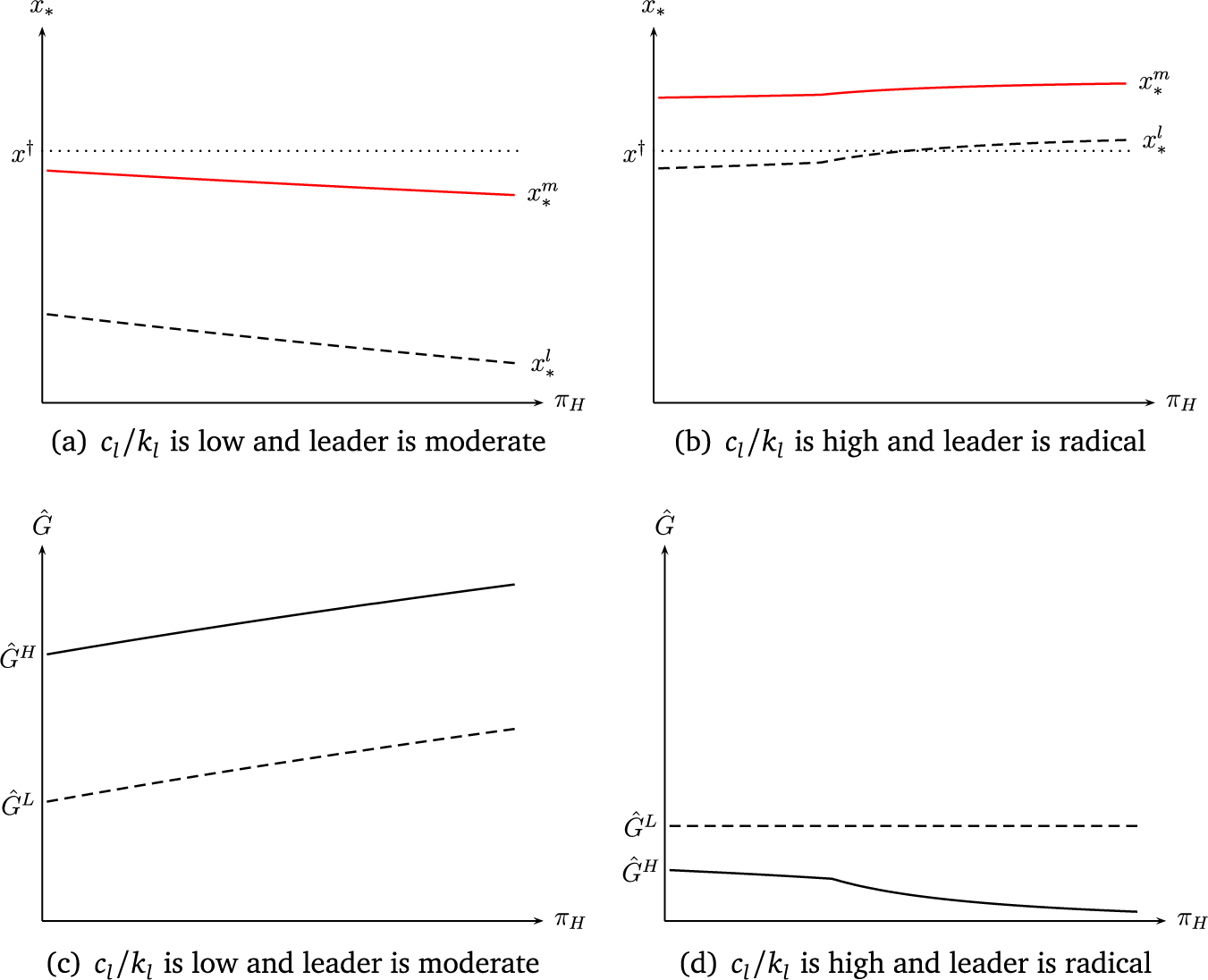




Comments
No Comments have been published for this article.