





Introduction
An earlier version of this paper was presented at EuMW 2025 and was published in its Proceedings [Reference Neuder, Schwarzbeck, Späth and Jiménez-Sáez1].
In the context of future communication standards, such as 6G and beyond, reconfigurable intelligent surfaces (RISs) have emerged as a solution for enabling reliable signal transmission with low latency and high data rates [Reference Liu, Liu, Xidong, Hou, Jiaqi, Di Renzo and Al-Dhahir2, Reference Björnson, Wymeersch, Matthiesen, Popovski, Sanguinetti and de Carvalho3]. These tunable surfaces promise to overcome challenges at millimeter-wave (mm-Wave) and terahertz (THz) frequencies, addressing the issue of limited signal coverage due to high path loss, increased absorption, and reduced scattering.
RIS can be envisioned as tunable reflectarrays, but without a defined feed. They consist of an array of radiating elements arranged in a grid, along with a tuning mechanism that enables dynamic control of wave propagation. In the far field, RIS can redirect electromagnetic waves toward desired directions, while in the near field, they can also focus waves on focal points. Figure 1 shows an outdoor scenario. Large-scale RIS, consisting of hundreds, thousands, or even millions of elements, are envisioned for future applications [Reference Björnson, Özdogan and Larsson4, Reference Zhang, Boya, Zhu Han and Song5]. Most commonly, semiconductor-based tuning mechanisms, such as PIN [Reference Dai, Wang, Wang, Yang, Tan, Shuangkaisheng, Shenheng, Yang, Chen, Di Renzo, Chae and Hanzo6] and varactor diodes [Reference Pei, Yin, Tan, Cao, Zhanpeng, Wang, Zhang and Björnson7], are used. While these technologies are readily available up to mm-Wave frequencies, they come with drawbacks, particularly in terms of power consumption and cost: Given that at least one diode is required per radiating element, semiconductor-based RIS quickly become prohibitively expensive as the array size increases [Reference Jiménez-Sáez, Asadi, Neuder, Delbari and Jamali8]. Micro-Electro-Mechanical Systems (MEMS) offer an alternative approach, enabling low power consumption and monolithic integration with antenna structures, providing few discrete phase states [Reference Bayraktar, Civi and Akin9]. However, MEMS-based solutions face challenges in reliability, response time, and require complex fabrication processes that limit scalability and cost-efficiency for large-area RIS [Reference Bayraktar, Civi and Akin9, Reference Jiménez Sáez, Asadi, Neuder, Wang and Jakoby10].
Exemplary outdoor scenario for a RIS [Reference Neuder, Schwarzbeck, Späth and Jiménez-Sáez1]. The different colors in the RIS qualitatively indicate different reflected phases at the radiating elements. LoS: Line of sight. RIS: Reconfigurable intelligent surface.

Figure 1 Long description
Reconfigurable intelligent surface setup with signal paths between a base station, RIS and users. At the top, a legend shows three signal paths: direct path in green, line of sight from base station to RIS in blue and line of sight from RIS to user in red. On the left, a detailed RIS setup is depicted, consisting of a control unit connected to a phase shifting layer and a radiating layer. On the right, a building is shown with the RIS attached to its side, redirecting signals from the base station to users. The base station is positioned on the left, with a blocked line of sight indicated by a dashed arrow pointing towards a user behind a wall. The RIS redirects signals over the wall to reach users, demonstrating its ability to overcome obstacles in signal transmission.
A promising alternative tuning mechanism is nematic liquid crystal (LC) [Reference Jiménez-Sáez, Späth, Neuder and Jakoby11]. Although it presents challenges such as moderate insertion losses, relatively slow response times, and temperature dependence, it also offers significant advantages. These include continuous tunability, transparency, low power consumption, and, most notably, large-scale scalability, making it a promising candidate for RIS applications. In [Reference Neuder, Späth, Schüßler and Jiménez-Sáez12], the delay line architecture (DLA) was proposed for LC-RIS. In contrast to conventional architectures relying on the detuning of a resonant element, called resonant architecture (RA), the DLA couples the incoming electromagnetic wave to a tunable LC-based phase shifter before retransmitting it into free space. The DLA allows LC-RIS to be optimized for low loss, fast response time, and wide bandwidth simultaneously. In [Reference Neuder, Späth, Schüßler and Jiménez-Sáez12], a DLA-based LC-RIS operating around 60 GHz is presented. The proposed LC-RIS is composed of 120 (12 $\times$10) tunable unit cell elements.
To demonstrate the scalability of the LC-RIS toward larger apertures, we extend our previously published 120-element design [Reference Neuder, Späth, Schüßler and Jiménez-Sáez12] to an array with 750 (25 $\times$30) elements, based on the same unit cell. In addition, this extended version of the conference paper [Reference Neuder, Schwarzbeck, Späth and Jiménez-Sáez1] addresses the following aspects: A novel measurement methodology enables a detailed characterization of the aperture efficiency. Furthermore, we perform fabrication tolerance modeling, systematically analyzing LC thickness variations and their impact on performance. Finally, an extensive comparative analysis is presented, offering a detailed comparison with state-of-the-art LC-RIS implementations (Table 1).
Comparison of LC-RIS realizations

Table 1 Long description
Comparison of multiple LC-RIS realizations by architecture and year, listing LC thickness, center frequency, bandwidth, element count, aperture efficiency, scan range, and maximum phase shift. Earlier RA entries from 2023 to 2025 span roughly 19.5 to 415 gigahertz, with bandwidth typically about 3.5 to 11 percent and scan ranges commonly about 30 to 120 degrees. Maximum phase shift for RA is usually around 200 to 320 degrees, with a few entries exceeding 360 degrees. Two DLA entries labeled as this work use about 4.6 micrometers LC thickness at about 59 gigahertz and report the largest bandwidth, about 24 percent, with scan ranges about 110 and 120 degrees and phase shift beyond 360 degrees. Aperture efficiency varies widely across designs, from low single digits up to the low 30 percent range, and several entries do not report efficiency. Some values are approximate or estimated, and several results are simulation-based, so cross-row comparisons should be treated as indicative rather than exact.
a Estimated from graphs.
b Might be larger. No more values provided.
c Dual polarized. Always minimum values shown regarding both polarizations.
d Combines resonant patches with resonant slots. Dual-band.
e Bandwidth and center frequency stated with regard to the definition in this work (-3 dB) at  $\theta_\mathrm{r} = 40^{\circ}$.
f Simulated.
The paper is structured as follows: First, the design of the proposed LC-RIS and its simulation results are presented. Subsequently, measurement results of the manufactured LC-RIS prototypes are evaluated. Thereby, the steering capabilities, the power consumption, and the response time are analyzed. Further, a measurement procedure for the aperture efficiency is proposed, and the impact of fabrication tolerances is modeled. Finally, the prototypes are compared to recent LC-RIS realizations to contextualize the potential of the DLA in comparison to the conventional RA.
Design and simulation results
The operating principle of the proposed LC-RIS is illustrated in Fig. 2(a). The setup consists of three main materials: the LC mixture, a glass substrate, and a conductor. An electromagnetic wave propagating in free space impinges on the aperture-coupled patch antenna, which couples the wave to an LC-based phase shifter through the slot. The wave propagates through the phase shifter to its open end, where the wave is reflected and subsequently re-radiated by the patch antenna. The unit cell elements are arranged in a triangular grid to facilitate sufficient space for the phase shifters. An element spacing 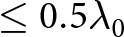 $\le 0.5\lambda_0$ is targeted to fully avoid the appearance of grating lobes, with
 $\lambda_0$ being the free-space wavelength.
Design and simulation results of the proposed LC-RIS [Reference Neuder, Schwarzbeck, Späth and Jiménez-Sáez1]. (a) Operation principle of the delay line architecture, the unit cell layout, and the side view of the LC-RIS. (b) Performance of the phase shifter in terms of losses (FoM) and compactness. The red dotted line indicates a compactness of 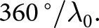 $360\,^{\circ}/\lambda_0.$ (c) Simulated co-polar aperture efficiency
 ${\eta_{Co}}$ in a 768 (
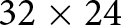 $\mathrm{32 \times 24}$) element RIS for a positive (pos.), and negative (neg.) steering angle
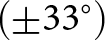 $(\pm 33^{\circ})$. LC: Liquid crystal. RIS: Reconfigurable intelligent surface. FoM: Figure of Merit.
 $\theta_\mathrm{r}$: reflected angle.

Figure 2 Long description
Three panels covering the LC-RIS delay line design, phase shifter metrics and beam steering simulation results. The first panel is a hardware architecture schematic labeled RIS dash Delay Line Architecture. It shows a unit cell in perspective view and side view. The layered structure includes a radiating layer, a phase shifting layer and an alignment layer. Materials identified in the legend are conductor, liquid crystal and glass. The side view labels the liquid crystal thickness as t subscript LC and a voltage label V subscript Sat is visible. The second panel is a dual-axis line chart labeled Phase shifter performance. The x-axis is labeled Frequency in gigahertz, ranging from 50 to 70 gigahertz. The left y-axis is labeled FoM in degree per decibel, where FoM stands for Figure of Merit and represents the phase shift achievable per unit of insertion loss. The left y-axis ranges from 0 to 100. The right y-axis is labeled Compactness in units of degree per lambda subscript 0, where lambda subscript 0 denotes free-space wavelength and this axis ranges from 0 to 480. Two curves are plotted. The FoM curve, read against the left axis, remains relatively flat across the frequency range, staying between approximately 75 and 100. The compactness curve, read against the right axis and shown as a solid orange line, increases as frequency increases, starting near 360 at 50 gigahertz and rising toward approximately 480 at 70 gigahertz. The third panel is labeled LC-RIS steering and contains two heatmaps and one line plot. The two heatmaps share the same axis structure. The x-axis of each heatmap is labeled theta subscript r in degrees, representing the reflected angle, ranging from negative 80 to positive 80 degrees. The y-axis is labeled Frequency in gigahertz, ranging from approximately 53 to 67 gigahertz. The colorbar on each heatmap is labeled eta subscript co in percent, where eta subscript co denotes co-polar aperture efficiency, ranging from 0 to 20 percent. In each heatmap, narrow vertical high-response bands appear at specific steering angles, with peak values near 15 to 20 percent. The left heatmap corresponds to negative steering and the right to positive steering, showing symmetric band positions at mirrored angles. The line plot to the right of the heatmaps shares the x-axis label theta subscript r in degrees from negative 80 to positive 80. The y-axis is labeled eta subscript co in percent, ranging from 0 to approximately 20 percent. Two curves are shown: one labeled Neg. for negative steering angle and one labeled Pos. for positive steering angle. Both curves show narrow peaks. The negative steering curve peaks at approximately negative 33 degrees and the positive steering curve peaks at approximately positive 33 degrees, each reaching near 18 percent efficiency. The two peaks are nearly symmetric about zero degrees.
The ellipsoidal shape of LC molecules allows continuous permittivity tuning via bias voltages, which control the orientation of the molecule director  $\vec{n}$ relative to the radio frequency (RF) electric field
 $\vec{E}_{RF}$ [Reference Jiménez-Sáez, Späth, Neuder and Jakoby11]. With the applied LC-mixture GT7-29001 from Merck Electronics KGaA, Darmstadt, Germany, the permittivity can be tuned between
 ${\varepsilon_{r,LC,\perp}}=2.46$ with
 ${tan\delta_{LC,\perp}}=0.0116$ and
 ${\varepsilon_{r,LC,\parallel}}=3.53$ with
 ${tan\delta_{LC,\parallel}}=0.0064$ at 19 GHz [Reference Fritzsch, Snow, Sargent, Klass, Kaur and Parri13]. For the glass substrate, AF32 from Schott is used (
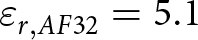 ${\varepsilon_{r,AF32}}=5.1$ and
 ${tan\delta_{AF32}}=0.009$ at 24 GHz [14]) and gold is employed as the conductor.
To maximize the phase shift per length and minimize the insertion losses, a defected ground structure inverted microstrip line (DGS-IMSL) topology is employed. The topology is well-suited for RIS applications [Reference Neuder, Wang, Schüßler, Jakoby and Jiménez-Sáez15] which require low insertion loss, fast response time, high compactness, and wide bandwidth. The simulated characteristics of the LC phase shifter are presented in Fig. 2(b). The (FoM) and the compactness are defined as:
 \begin{equation}
\begin{alignedat}{4}
\mathrm{FoM} &{}= \frac{\Delta \phi_\mathrm{max}}{\mathrm{IL_{max}}}
\qquad
\mathrm{Compactness} &{}= \frac{\Delta\phi_\mathrm{max}\, \lambda_0}{l_\mathrm{phys}}
\end{alignedat}
\end{equation}
where  ${\Delta \phi_\mathrm{max}}$,
 $\mathrm{IL_\mathrm{max}}$ and
 $l_\mathrm{phys}$ represent the phase shifter’s max. differential phase shift, max. insertion loss and physical length, respectively. An FoM of
 ${80}^{\circ}/\mathrm{dB}$ corresponds to 4.5 dB loss for
 ${360}^{\circ}$ phase shift and a compactness of
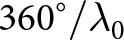 ${360}^{\circ}/\lambda_0$ corresponds to a phase shift of
 ${360}^{\circ}$ differential phase shift per
 ${0.5}\,{\lambda_0}$, as the wave travels back and forth through the phase shifter. The maximum tuning range is
 $470^{\circ}$ at 60 GHz, which satisfies the requirements for the desired steering capabilities. The temperature-dependent behavior of LC is not studied in this work; however, the used LC mixture was characterized in [Reference Tesmer, Razzouk, Polat, Wang, Jakoby and Maune16] and [Reference Späth, Neuder, Sode, Schüßler, Jakoby and Jiménez-Sáez17], which revealed a slight degradation of the achievable differential phase shift with increasing temperature.
The thickness of the LC layer,  $\mathrm{t_\mathrm{LC}}$, and the glass substrate are
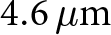 ${4.6}\,{\mu \mathrm{m}}$ and
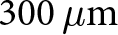 ${300}\,{\mu \mathrm{m}}$, respectively. A thin LC layer is essential, as the response times
 ${\tau_{on}}$ (transition from
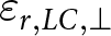 ${\varepsilon_{r,LC,\perp}}$ to
 ${\varepsilon_{r,LC,\parallel}}$) and
 ${\tau_{off}}$ (transition from
 ${\varepsilon_{r,LC,\parallel}}$ to
 ${\varepsilon_{r,LC,\perp}}$) increase with
 ${t_\mathrm{LC}^2}$ [Reference Jakoby, Gaebler and Weickhmann18]. To facilitate a faster transition of the molecule orientation back to its initial state after the bias is removed, a grooved alignment layer is applied to the surfaces. Furthermore, an electrically thick glass substrate is required to achieve a large relative bandwidth. The gold layers have a thickness of
 ${2}\,{\mu \mathrm{m}}$. The element spacing for the proposed LC-RIS is
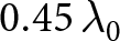 ${0.45}\,{\lambda_0}$ within the triangular grid. All relevant unit cell dimensions can be found in Fig. 1 of the supplementary material.
The simulated beam-steering capabilities of the proposed LC-RIS are demonstrated in Fig. 2(c). The RIS is simulated comprising 768Footnote 1 (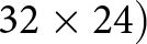 $\mathrm{32 \times 24})$ unit cell elements. The structure is excited by a plane wave impinging from broadside. The simulation setup is described in more detail in [Reference Neuder, Díaz-Rubio, Liu, Dzieia, Wang and Jiménez-Sáez19]. The displayed results show the beam-steering in the H-plane, targeting angles around
 $\pm{33^{\circ}}$. The aperture efficiency
 ${\eta_{Co}}$ is evaluated relative to a perfectly conducting metal plate at the same distance, and peaks at 21.5%. The primary sources of loss originate from the lossy materials, contributing 28.6% (gold), 21.4% (LC), and 18.2% (AF32) at 60.75 GHz. Outside its operating frequency, the LC-RIS behaves similarly to a metal plate, leading to a strong reflection at
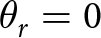 ${\theta_r=0}$. Figure 2 of the supplementary material provides simulation results showing the magnitude and phase response of the unit cell.
Measurement results
Two LC-RIS are fabricated based on the unit cell above using standard lithographic processes [Reference Neuder, Späth, Schüßler and Jiménez-Sáez12]. SU-8 photoresist has been applied for the spacers between the two glass substrates constituting the LC layer thickness,  $t_\mathrm{LC}$. The smaller prototype with 120 (
 $\mathrm{10 \times 12}$) elements has already been analyzed in [Reference Neuder, Späth, Schüßler and Jiménez-Sáez12]. In addition, a larger prototype with 750 (
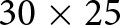 $\mathrm{30 \times 25}$) elements is manufactured. Figure 3(a) displays both prototypes and the measurement setup. See [Reference Neuder, Späth, Schüßler and Jiménez-Sáez12] for a detailed description of the setup. Reference measurements are taken and subtracted to isolate the RIS from the cluttered environment. In the following, the measured characteristics of the LC-RIS prototypes are analyzed.
Measurement of the proposed LC-RIS [Reference Neuder, Schwarzbeck, Späth and Jiménez-Sáez1]. (a) Front and back view of the LC-RIS with 120 and 750 elements and the measurement setup. (b) Normalized measurement of the beam-steering capabilities of the 120-element RIS. (c) Normalized measurement of the beam-steering capabilities of the 750-element RIS. The dashed line in the right heat map indicates the impact of beam-squinting. RIS: Reconfigurable intelligent surface. LC: Liquid crystal. Tx: Transmitting antenna. Rx: Receiving antenna.  $\theta_\mathrm{r}$: Reflected angle. VNA: Vector network analyzer.

Figure 3 Long description
Three top-row sections. Left section labeled Front view shows two rectangular boards labeled 120 element RIS and 750 element RIS, each with a dense grid of small square elements. Middle section labeled Back view shows two rectangular boards labeled 120 element RIS and 750 element RIS, with a large rectangular area and a connector area on the bottom side of the larger board. A small inset labeled Unit cell shows a close-up with several vertical and horizontal lines and arrows. Right section shows a measurement setup with labels Meas. setup, Voltage supply, VNA, Tx, Rx, Turntable and RIS. The image B showing a row labeled 120 element RIS at 61 GHz with three plots. Left plot is a line graph with y-axis label Magnitude (decibel) and x-axis label theta r (degree). The x-axis ranges from minus 60 to 60. The y-axis ranges from minus 15 to 0. A legend lists minus 60 degree, minus 50 degree, minus 40 degree, minus 30 degree, minus 20 degree, 20 degree, 30 degree, 40 degree, 50 degree and 60 degree. Multiple narrow peaks appear at different theta r positions across the range, with peak magnitudes reaching near 0 to -5 decibel and minima near minus 15 decibel. Middle plot is a heat map titled Steering to: minus 40 degree. The y-axis label is Frequency (gigahertz) ranging from 53 to 67. The x-axis label is theta r (degree) ranging from minus 60 to 60. The color scale at the right is labeled Magnitude (decibel) with tick labels 0, minus 5, minus 10 and minus 15. Bright regions form a main lobe centered near theta r around minus 40 degree across a band of frequencies, with additional weaker streaks at other angles. Right plot is a heat map titled Steering to: plus 40 degree with the same axes and scale: Frequency (gigahertz) 53 to 67, theta r (degree) minus 60 to 60 and Magnitude (decibel) ticks 0, minus 5, minus 10, minus 15. Bright regions form a main lobe centered near theta r around plus 40 degree across a band of frequencies. The image C showing a row labeled 750 element RIS at 60 GHz with three plots. Left plot is a line graph with y-axis label Magnitude (decibel) and x-axis label theta r (degree). The x-axis ranges from minus 60 to 60. The y-axis ranges from minus 15 to 0. The legend lists minus 60 degree, minus 50 degree, minus 40 degree, minus 30 degree, minus 20 degree, 20 degree, 30 degree, 40 degree, 50 degree and 60 degree. Multiple narrow peaks appear at different theta r positions, with several peaks reaching near 0 to -5 decibel and troughs near minus 15 decibel. Middle plot is a heat map titled Steering to: minus 40 degree. The y-axis label is Frequency (gigahertz) ranging from 54 to 66. The x-axis label is theta r (degree) ranging from minus 60 to 60. The color scale is labeled Magnitude (decibel) with tick labels 0, minus 5, minus 10 and minus 15. A bright main lobe is centered near theta r around minus 40 degree across a band of frequencies, with additional weaker streaks at other angles. Right plot is a heat map titled Steering to: plus 40 degree with the same axes and scale: Frequency (gigahertz) 54 to 66, theta r (degree) minus 60 to 60 and Magnitude (decibel) ticks 0, minus 5, minus 10, minus 15. A bright main lobe is centered near theta r around plus 40 degree across a band of frequencies.
Steering capabilities and bandwidth
The fabricated LC-RIS supports beam-steering in only one plane, due to a limitation to column-wise biasing. Note that this limitation is purely technological, as element-wise biasing is already implemented in LC-displays [Reference Neuder, Späth, Schüßler and Jiménez-Sáez12, Reference Rose, Chen, Cranton and Fihn20, Reference Widmaier, Hanghang, Dettling, Baur, Fruehauf, Mohamed, Keusgen, Otto and Jost21]. Beam-steering is achieved by applying 1 kHz square-wave bias voltages between 0 and  $\mathrm{20\,V_{pp}}$. The bias lines are located on the lower glass substrate next to the microstrip lines of the phase shifters, they are visible in the microscope photo of the unit cell in Fig. 3(a). The triangular RF chokes are
 $\lambda$/4-stubs, which decouple the biasing from the RF signal. All column bias lines are routed out on both sides of the RIS, and the slightly different sizes of the glass substrates allow for contacting the bias line pads. On one side, cables have been soldered on for connection with the DAC providing the bias voltages.
In Fig. 3(b) and (c), the measured steering capabilities of the 120- and 750-element LC-RIS can be found. The beam-steering of the large RIS is comparable to the simulation results in Fig. 2(c), but lacks the reflection to 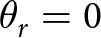 ${\theta_r=0}$, as the latter is subtracted by the reference measurements. Both prototypes exhibit beam-steering capabilities between
 $-60^{\circ}$ and
 $+60^{\circ}$ and a -3 dB bandwidth between 9% (small prototype) and 9.5% (large prototype), proving the scalability of the design. The bandwidth is evaluated corresponding to the reflected power at an exemplary angle
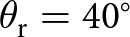 $\theta_\mathrm{r}=40^{\circ}$, corrected for beam-squinting to prevent underestimation in narrow beams.
Power consumption and response time
Although not optimized for low power consumption, one LC-RIS element consumes only 21.5 nW on average, measured using an E4980A Precision LCR Meter. Hence, for a RIS with  $\mathrm{10^6}$ elements (2.5 m x 2.5 m aperture with
 ${\lambda_0/2}$ spacing at 60 GHz), the total power consumption would be 21.5 mW. The response times of an LC phase shifter with
 $t_\mathrm{LC}={4.6}\,{\mu \mathrm{m}}$ is measured to
 $\tau_\mathrm{on} = {15}\,{ms}$ and
 $\tau_\mathrm{off} = {72}\,{ms}$ [Reference Neuder, Wang, Schüßler, Jakoby and Jiménez-Sáez15]. The measured total response time of the larger LC-RIS prototype is
 $\tau_{\mathrm{RIS}}\approx{250}\,{ms}$, which is higher than expected. The undesired increase most probably arises from a non-ideal structuring of the alignment layer [Reference Neuder, Späth, Schüßler and Jiménez-Sáez12]. By solving these technological imperfections, response times of only a few tens of milliseconds may be attained [Reference Jakoby, Gaebler and Weickhmann18].
Aperture efficiency
The aperture efficiency  $\eta_\mathrm{Co}$ represents how effectively the physical aperture of the RIS contributes to the desired backscattered wave, both in terms of steering direction and polarization purity. Losses occur as portions of the incident power are dissipated as heat within the device materials (glass, gold, and LC) or excite scattering modes that lead to differing polarizations or radiation into undesired directions. The aperture efficiency can be defined relative to the ideal reflection from a perfectly conducting metal plate of the same aperture size, for which the radar cross section (RCS) can be determined analytically:
 \begin{equation}
{\sigma_{\text{MP}} = \frac{\text{4}\pi {\text{A}}^2_{\text{MP}}\text{cos}(\theta_{\text{Tx}}){\text{cos}}(\theta_{\text{Rx}}){\text{cos}}(\phi_{\text{Tx}}){\text{cos}}(\phi_{Rx})}{\lambda_0^2}} ,
\end{equation}
where  $\mathrm{A_{MP}}$ corresponds to the aperture size of the metal plate and
 ${\theta_{\text{Rx/Tx}}}$ and
 ${\phi_{\text{Rx/Tx}}}$ correspond to the angles of incoming and reflected waves with respect to the metal plate. Based on the measurement of the received powers for the RIS and the metal plate, i.e., the scattering parameters
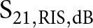 $\mathrm{S_{21,RIS,dB}}$ and
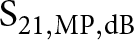 $\mathrm{S_{21,MP,dB}}$, and the analytically calculated RCS of the metal plate, the RIS RCS
 ${\sigma_{RIS}}$ is calculated according to
 \begin{equation}
{\sigma_{\text{RIS}} = \sigma_{\text{MP}} + {\text{S}}_{\text{21,RIS,dB}} - {\text{S}}_{\text{21,MP,dB}}}.
\end{equation}
With this result, the aperture efficiency of the RIS is given by
 \begin{equation}
{\eta_{\text{Co,meas}} = \frac{\lambda_0^2 \sigma_{\text{RIS}}}{4\pi {\text{A}}_{\text{RIS}}^2{\text{cos}}(\theta_{\text{Tx}}){\text{cos}}(\theta_{\text{Rx}}){\text{cos}}(\phi_{\text{Tx}}){\text{cos}}(\phi_{\text{Rx}})}},
\end{equation}
where  ${\theta_{\text{Rx}}}$,
 ${\theta_{\text{Tx}}}$,
 ${\phi_{\text{Rx}}}$ and
 ${\phi_{\text{Tx}}}$ are the incoming and reflected angles in azimuth and elevation with respect to the RIS.
 $\mathrm{A_{RIS}}$ is the aperture size of the RIS, calculated as
 \begin{equation}
\mathrm{A_{RIS} = d_x \, d_y \, M \, N},
\end{equation}
with  $\mathrm{d_x}$ and
 $\mathrm{d_y}$ being the element spacings and M and N the number of rows and columns. Theoretically, a metal plate with an arbitrary aperture size can be taken for evaluation since the aperture of the surface is included in Eq. 2. However, using a metal plate with dimensions matching those of the RIS is preferable, as it helps minimize the effects caused by variations in the illuminated areas of the horn antennas’ beam widths, i.e., the same illumination efficiency. Just like the RIS measurements, the metal plates are evaluated with subtraction of a reference measurement to isolate their response from the environment. The measurement setup for the aperture efficiency can be seen in Fig. 3 of the supplementary material.
The aperture efficiency of the small RIS prototype is illustrated in Fig. 4. It features a maximum simulated aperture efficiency of 17.2 %. This value is lower than the 21.5 % found by the simulation results in the previous section, arising from the additional consideration of the RF choke compared to the ideal model used before. The effect of beam-squinting on the reflection angle  ${\theta_r}$ is almost negligible due to the small aperture size as well as the rather small steering angle, which is confirmed by simulations. The measured aperture efficiency (blue) with a peak of 9.2 % is considerably lower than the simulation results. Additionally, the measured bandwidth shows a reduction with respect to the simulations. The missing specular reflection in measurements also becomes evident, which is a side-effect of the reference measurement subtraction as explained in [Reference Neuder, Späth, Schüßler and Jiménez-Sáez12].
Aperture efficiency results of the RIS prototype with 120 elements.

Figure 4 Long description
Image A showing a top view of a square device with a grid of small square features inside a square border. Image B showing a line graph with four curves and a legend. The x-axis is labeled Frequency (GHz), ranging from 53 to 67 with labeled ticks at 54, 57, 60, 63 and 66. The y-axis is labeled eta Co (percent), ranging from 0 to 25 with labeled ticks at 0, 5, 10, 15, 20 and 25. The legend lists Sim asterisk, Sim #, Sim #+ and Meas#. The Sim asterisk curve rises from near 0 at 53 GHz to about 10 at 57, about 15 at 60, about 17 at 61, then decreases to about 8 at 63, about 4 at 66 and near 0 at 67. The Sim # curve rises from near 0 at 53 to about 8 at 57, about 15 at 60, then decreases to about 14 at 62, about 8 at 64 and near 0 at 66. The Sim#+ curve rises from near 0 at 54 to about 2 at 56, about 2 at 58, about 9 at 60, then decreases to about 8 at 62, about 3 at 64 and near 1 at 66. The Meas# curve rises from near 0 at 54 to about 1 at 56, about 4 at 58, about 8 at 60, then decreases to about 5 at 63, about 3 at 64 and near 0 at 67. Asterisk: Considers beam-squint, Plus: Considers fabrication tolerances, #: Does not consider beam-squint. Image C showing a heatmap labeled Sim. The x-axis is labeled theta r (degree), ranging from minus 40 to 60 with labeled ticks at minus 40, minus 20, 0, 20, 40 and 60. The y-axis is labeled Frequency (GHz), ranging from 55 to 65 with labeled ticks at 56, 58, 60, 62 and 64. A vertical color scale at the right is labeled eta Co (percent), ranging from 0 to 20 with labeled ticks at 0, 5, 10, 15 and 20. The heatmap shows two narrow high-intensity vertical bands centered near theta r about 0 to 10 degrees and around 40 degrees across much of the frequency range, with the strongest region around frequencies near 60 to 62. Image D showing a heatmap labeled Meas. The x-axis is labeled theta r (degree), ranging from minus 40 to 60 with labeled ticks at minus 40, minus 20, 0, 20, 40 and 60. The y-axis is labeled Frequency (GHz), ranging from 55 to 65 with labeled ticks at 56, 58, 60, 62 and 64. A vertical color scale at the right is labeled eta Co (percent), ranging from 0 to 20 with labeled ticks at 0, 5, 10, 15 and 20. The heatmap shows a narrow high-intensity region near theta r around 40 degrees, concentrated mainly around frequencies near 60 to 62, with weaker intensity away from that region.
The outcome for the prototype with 750 elements is illustrated in Fig. 5. The results reveal a much lower measured aperture efficiency with a maximum of approximately 2.6 %. The maximum aperture efficiency obtained in simulation is 15.7 %. Due to the larger aperture size, the results show a comparatively more pronounced effect of beam-squinting, both in simulation and measurement.
Aperture efficiency results of the RIS prototype with 750 elements.

Figure 5 Long description
750 element prototype Top-left: A rectangular device view with a dense grid of small square elements inside a frame. A scale bar below reads 10 mm for scale reference. Bottom-left: Line graph with three curves. The x-axis label is Frequency (GHz), with ticks at 54, 57, 60, 63 and 66. The y-axis label is eta subscript CO (percent), ranging from 0 to 25 with ticks at 0, 5, 10, 15, 20 and 25. A legend lists Sim asterisk, Sim # and Meas#. Sim asterisk is a dashed curve that rises from about 2 at 54, reaches about 15 near 60, then drops to about 2 by 64. Sim # is a dotted curve that rises from about 0 at 54, peaks near 16 around 61, then decreases to about 1 by 66. Meas # is a solid curve that stays near 0 to about 1 from 54 to 58, rises to about 3 near 60, then decreases toward about 0 by 66. Top-right: Heatmap labeled Sim. The x-axis label is theta r (degree), ranging from minus 40 to 60 with ticks at minus 40, minus 20, 0, 20, 40 and 60. The y-axis label is Frequency (GHz), ranging from 55 to 65 with ticks at 56, 58, 60, 62 and 64. A vertical color scale at the right is labeled eta subscript Co (percent), ranging from 0 to 20 with ticks at 0, 5, 10, 15 and 20. Two narrow high-intensity vertical bands appear near theta r about 0 and about 30 across much of the frequency range. Bottom-right: Heatmap labeled Meas. The x-axis label is theta r (degree), ranging from minus 40 to 60 with ticks at minus 40, minus 20, 0, 20, 40 and 60. The y-axis label is Frequency (GHz), ranging from 55 to 65 with ticks at 56, 58, 60, 62 and 64. A vertical color scale at the right is labeled eta subscript Co (percent), ranging from 0 to 20 with ticks at 0, 5, 10, 15 and 20. One narrow high-intensity vertical band appears near theta r about 30 across much of the frequency range.
Impact of fabrication tolerances
Regarding the considerable reduction of the aperture efficiency and the smaller bandwidths, two possible causes may be considered: i) increased material loss and ii) fabrication tolerances. The impact of i) is presumably rather small, since the same materials showed a good agreement between simulation and measurement (in [Reference Neuder, Späth, Schüßler and Jiménez-Sáez12] and [Reference Neuder, Wang, Schüßler, Jakoby and Jiménez-Sáez15]). Hence, ii) fabrication tolerances are assumed to have a major impact on the measured performance. Particularly, an uneven LC thickness (see Fig. 2(a)) and misalignments between the metallization layers are supposed to affect the measured outcome.
To verify this assumption, first, the distribution of the back-scattered power in azimuth and elevation is examined for both prototypes in Fig. 6. The aim is to analyze whether the LC-RIS produce a focused beam (as desired) or whether they scatter the incoming energy to various directions. Within this context, an initial bias voltage set, which considers a uniform  $t_\mathrm{LC} = {4.6}\,{\mu \mathrm{m}}$ layer, is compared to a bias voltage set that is optimized toward maximum received power [Reference Neuder, Späth, Schüßler and Jiménez-Sáez12]. Through an optimization of the bias voltages for the desired steering angle, fabrication tolerances, such as an uneven
 $t_\mathrm{LC}$ across the surface, can be compensated to a certain extent, improving the focusing capabilities of the RIS.
Measured distribution of back-scattered power of the RIS prototypes over azimuth and elevation for an initial voltage distribution and an optimized voltage distribution. Each graph is normalized to its respective maximum.

Figure 6 Long description
Four heatmap plots display the distribution of back-scattered power for two different prototypes, each with initial and optimized voltage settings. The top row represents the 120 element prototype, while the bottom row shows the 750 element prototype. Each plot has the azimuth angle labeled theta subscript r in degrees on the x-axis, ranging from -40 to 60 degrees and the elevation angle labeled phi subscript r in degrees on the y-axis, ranging from -60 to 60 degrees. The color scale on the right indicates magnitude in decibels, ranging from -15 to 0. The initial voltage distribution plots show a more dispersed scattering pattern, while the optimized voltage distribution plots exhibit a more focused beam pattern. The optimized settings result in a concentrated area of higher magnitude, indicating improved focusing capabilities.
Considering the smaller prototype, the reflected beam seems to be well focused for the reflection for the set of initial bias voltages (upper left subplot). However, angular offsets are present, as the device was intended to steer toward 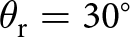 $\theta_\mathrm{r} = 30^{\circ}$ (azimuth), but shows its maximum at
 $\approx42^{\circ}$. Furthermore, since the elevation plane does not offer steering capabilities, the beam would ideally steer toward
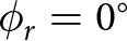 $\phi_r = 0^{\circ}$, but is found at
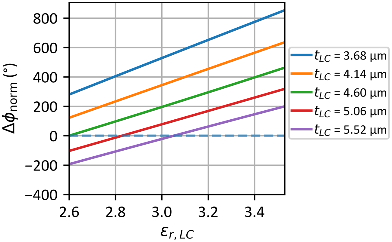
 $28^{\circ}$. Since the offsets are consistent for all steering angles, they are expected to arise from the impact of a non-uniform, tilted LC thickness that increases toward one corner of the surface. The simulated effect of varying
 $t_\mathrm{LC}$ on the resulting phase of a unit cell is shown in Fig. 7. In essence, the plot shows that, given a fixed LC permittivity, the differential phase shift is significantly affected by even small variations in LC thickness. The impact of this is studied in the supplementary material in more detail, where a model shows that the tilted LC surface reduces the maximum magnitude by
 $\approx {3}\,{dB}$. Hence, the uneven LC thickness is assumed to be the major reason for the overall decreased aperture efficiency. For the small prototype, the voltage optimization barely increases the maximum received magnitude by
 $\approx {0.3}\,{dB}$.
Influence of varying  $t_\mathrm{LC}$ (see Fig. 2) on the inter-element phase shift
 $\Delta \phi$. The phase shifts are presented with regard to the unbiased case (
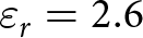 ${\varepsilon_r}=2.6$) with thickness
 $t_\mathrm{LC}={4.6}\,{\mu \mathrm{m}}$.

Similar to the lower aperture efficiency, the decreased bandwidth of the small prototype is most likely due to fabrication imperfections, especially due to a slightly misaligned upper and lower glass substrate. Simulations show that a misalignment ( $\le30\,\mu m$) between the metallization (ground plane, phase shifter and antennas) does not have a decisive influence on the maximum aperture efficiency, but rather on the bandwidth. Together with the tilted LC layer thickness, this effect is considered in the orange curve in Fig. 4, which agrees well with the measurement results. It should be noted that the model, which has been adjusted to align with the measurement results, is intended to illustrate the potential impact of fabrication tolerances rather than provide an accurate representation of the fabricated prototype.
The lower left subplot of Fig. 6 shows the initial back-scattered power of the larger 750-element prototype with the bias voltages set to steer toward 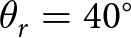 $\theta_r=40^{\circ}$. No distinct main beam is present, but the wave is scattered to various directions without a clear focus. The behavior is assumed to also result from a non-uniform
 $t_\mathrm{LC}$, which appears to vary randomly across the surface (see the supplementary material). Nonetheless, through the optimization process, the beam could be directed to the desired direction, such that the main lobe intensity is increased by more than
 $6\,\mathrm{dB}$ in comparison to the initial voltage set. Note, however, that the voltages can only be optimized in one plane for the given prototype, such that the result is still well below the optimum. Hence, it can be stated that the beam is not ideally focused toward the desired direction, which is also the main reason for the comparably low aperture efficiency
 $\eta_\mathrm{Co}$ shown in Fig. 5.
For a more detailed assessment of the impact of LC thickness on the measurement results, extended simulations are provided in the supplementary material. The results reveal that a variation of the LC layer thickness has a considerable impact on the beamforming performance of a RIS. In particular, a high fluctuation across the surface poses a significant challenge. Excess glue, non-uniform SU-8 photoresist spacers, and dust particles are the main causes of the thickness variations. A bias voltage optimization can help to mitigate the negative effects in laboratory environments, but it may not be practical for real-world RIS deployments with thousands or millions of elements because the required optimization time becomes excessive. However, the achievement of uniform  $t_\mathrm{LC}$ for large-scale RIS is merely a technological challenge and has already been solved for LC display applications.
Comparison
To contextualize the results from this paper, the presented prototypes are compared to several recent reflect-type LC-RIS implementations from the literature in Table 1. Note, however, that one or several specifications are often not directly provided in the literature, which is why they must be interpreted from graphs. When comparing the LC-RIS realizations, several observations can be made regarding the following key aspects.
Type: The RA remains the most popular architecture for the design of LC-RIS, with only one prototype in the literature also employing a DLA approach.
LC layer thickness: To achieve a few percent of bandwidth, RA-based prototypes generally require thicker LC layers [Reference Neuder, Späth, Schüßler and Jiménez-Sáez12] than those utilizing the DLA, leading to significantly slower response times. Nevertheless, the results in the table indicate that operating at higher frequencies enables the RA-based prototypes to use thinner LC layers, thanks to the shorter wavelengths. In contrast, the DLA approaches feature thinner  $\mathrm{t_\mathrm{LC}}$ also at lower frequencies, as the layer thickness has a much smaller impact on its performance when employing an appropriate phase shifter topology [Reference Neuder, Späth, Schüßler and Jiménez-Sáez12]. An exception is prototype number 9, which is based on the RA, but features
 $\mathrm{t_\mathrm{LC}}={10}\,{\mu \mathrm{m}}$ at 28 GHz. This is accomplished by using patches placed on top of resonant cross-slot structures, enabling the thin
 $t_\mathrm{LC}$ while maintaining good functionality.
Bandwidth: Before comparing the bandwidths, it must be noted that the latter is not stated directly in any of the literature sources. Hence, due to the lack of data, it could not be estimated as the -3 dB bandwidth as defined in this paper. The only metric for which the bandwidth could be compared is the variation of the differential RIS induced phase shift over frequency. For this purpose, the bandwidth is defined as the frequency range in which the differential phase shift,  $\Delta \phi_\mathrm{max}$, does not differ more than 25% from the value at its center frequency, which was defined in [Reference Neuder, Díaz-Rubio, Liu, Dzieia, Wang and Jiménez-Sáez19]. However, it must be noted that this definition neglects the impact caused by the frequency-dependent amplitude of the reflection, for example due to the limited bandwidth of the radiating element.
According to the utilized metric, the bandwidth of the prototypes introduced in this work is significantly higher than that of the prototypes found in the literature. This is primarily due to the choice of architecture. Specifically, the RA-based prototypes feature limited bandwidths because of the frequency dependence of their phase profile, which is characteristic of their resonant nature. In this context, prototype 6 is also expected to demonstrate a wide bandwidth, although the paper does not provide enough data to confirm this.
Loss: Compared to the efficiencies of the RA, the measured aperture efficiencies of the prototypes presented in this work are considerably lower. Yet, two aspects must be noted: First, with one exception, all realizations of the RA type, for which the aperture efficiency can be determined, employ substantially thicker LC layers. With micrometer-thin LC layers, their efficiency would drastically degrade. Second, all the competing realizations use glass substrates with substantially lower loss (e.g., quartz glass, which is not suitable for RIS with large apertures) and most use copper, which poses a significant difference to the materials used in this work, which are gold and comparably high-loss glass (tan $\delta = 0.011$ versus tan
 $\delta = 0.0009-0.002$).
The only RA approach with comparable LC thickness (prototype 9) compared to the prototypes presented in this paper, though still more than twice as thick, likewise demonstrates a lower aperture efficiency than the small prototype. On top of that, the architecture and unit cell proposed in this work demonstrate the potential for high-efficiency LC-RIS, with simulations showing that efficiencies above 40 % are achievable when low-loss materials are utilized, and significant fabrication tolerances are excluded.
Scan and phase range: Most of the RA implementations have limited phase ranges of less than  $360^{\circ}$, which could reduce the beamforming capabilities of the LC-RIS. In contrast, the DLA approaches can achieve a phase range exceeding
 $360^{\circ}$. The scan ranges are primarily determined by the radiating elements. While most of the competing implementations do not demonstrate beam steering at larger angles (
 $ \gt 40^{\circ}$), they are expected to be capable of steering toward these angles as well.
To conclude, while the conventional RA-based prototypes do not allow for simultaneous optimization of loss, bandwidth, and response time, prototype 9 emerges as the strongest RA-based competitor. By increasing the complexity of its design by introducing resonant slots in its ground plane, it features a thin LC layer and combines it with dual-band and dual-polarization functionality. Still, the comparison highlights the superior potential of DLA approaches, which promises micrometer-thin LC layers, broad bandwidth, and the possibility of low-loss performance, in addition to exceptional versatility thanks to their wide phase range. The prototypes developed in this work reinforce these findings.
Conclusion
This paper presents the realization of two 60 GHz LC-RIS prototypes with 120 and 750 elements that are based on planar LC phase shifters, i.e., the delay line architecture. The RISs incorporate a thin 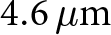 ${4.6}\,{\mu \mathrm{m}}$ LC-layer, demonstrating beam-steering capabilities of
 ${\pm60^{\circ}}$, -3 dB bandwidths exceeding 9% and a measured aperture efficiency of more than 9%. While fabrication constraints impact the performance, this work confirms
I) The scalability of the LC-RIS, as such challenges have already been effectively addressed in large-scale LC-display manufacturing.
II) The superior potential of designing LC-RIS based on the delay line architecture in contrast to the conventional resonant architecture, particularly regarding the trade-off between bandwidth, efficiency, and response time.
Supplementary material
The supplementary material for this article can be found at https://doi.org/10.1017/S1759078726103602.
Acknowledgements
We thank Merck Electronics KGaA, Darmstadt, Germany, for providing the liquid crystal mixture.
Funding statement
This work was funded by the Deutsche Forschungsgemeinschaft (DFG, German Research Foundation) - Project-ID 287022738 - TRR 196 MARIE within project C09.
Competing interests
The authors declare none.

Julia Schwarzbeck received the B.Sc. degree in electrical engineering and information technology from TU Darmstadt, Germany, in 2024, with a focus on microwave engineering and communication technology. She is currently pursuing her M.Sc. degree in electrical engineering and information technology at the Technical University of Munich. Her current research interests include antennas, reconfigurable intelligent surfaces and microwave measurements.

Robin Neuder received the B.S. and M.S. degree in electrical engineering and information technology from TU Darmstadt, Germany in 2019 and 2021, respectively. Since 2021, he has been a Research Assistant with the Institute of Microwave Engineering and Photonics at TU Darmstadt. His research interests include compact liquid-crystal based tunable planar devices and their integration into Reconfigurable Intelligent Surfaces.

Marc Späth received the B.Sc. and M.Sc. degrees in 2020 and 2022, respectively, in electrical engineering and information theory from Technical University Darmstadt, Darmstadt, Germany, where he is currently working towards the Ph.D. degree with the Microwave Engineering Group. His current research interests include tunable microwave filters and phase shifters based on liquid crystal technology and material characterization.

Alejandro Jiménez-Sáez (S’15, M’22) received the master’s degrees (Hons.) in telecommunications engineering from the Polytechnic University of Valencia, Spain, and in electrical engineering from the Technical University of Darmstadt, Germany, in 2017. In 2021, he received the Dr.-Ing. degree (with distinction) in electrical engineering from the TU Darmstadt and the Freunde der TU Darmstadt prize for the best dissertation in electrical engineering. He obtained the Athene Young Investigator award at TU Darmstadt and leads the Smart RF Systems based on Artificial and Functional Materials independent research group. His current research interests include chipless RFID, electromagnetic bandgap structures, liquid crystal, and reconfigurable intelligent surfaces.




 Open access

