Implications
This paper describes an up-to-date stochastic reproduction model of Holstein dairy cows. This model is sensitive to both milk production and body reserves and takes into account the recent evolutions of reproductive performance in dairy cows. This model is able to well simulate the overall reproductive performance observed in commercial farms. Therefore, it can be used in dynamic individual-based herd simulation models to anticipate the consequences of management strategies (in terms of reproduction or feeding) on dairy herd demography and global performance.
Introduction
Individual-based herd models, which individually describe each single animal, are a valuable and widely used solution for anticipating milk production responses to management practices. The lactation stage is a key driver of individual milk production in dairy cows, and the demography of the herd is a key driver of the herd milk production. However, in most of the current dairy herd production models, the representation of the reproductive process is usually either oversimplistic, using fixed calving to ovulation intervals or fixed cycle length of 21 days (Allore et al., Reference Allore, Schruben, Erb and Oltenacu1998; Blanc et al., Reference Blanc, Martin and Bocquier2001; Blanc and Agabriel, Reference Blanc and Agabriel2008), or well out of date relative to modern dairy genotypes (Oltenacu et al., Reference Oltenacu, Milligan, Rounsaville and Foote1980; Dijkhuizen et al., Reference Dijkhuizen, Stelwagen and Renkema1986; Plaizier et al., Reference Plaizier, King, Dekkers and Lissemore1998), where 15% to 30% of the cycles are affected by prolonged luteal phase (PLP) (Grimard and Disenhaus, Reference Grimard and Disenhaus2005), duration of normal cycles has increased (Sartori et al., Reference Sartori, Haughian, Shaver, Rosa and Wiltbank2004) and oestrus expression (Kerbrat and Disenhaus, Reference Kerbrat and Disenhaus2004; Roelofs et al., Reference Roelofs, Lopez-Gatius, Hunter, van Eerdenburg and Hanzen2010) and conception rate (Lucy, Reference Lucy2001; Grimard et al., Reference Grimard, Fréret, Chevallier, Pinto, Ponsart and Humblot2006) have strongly decreased. More recently, a dynamic simulation model was developed by Inchaisri et al. (Reference Inchaisri, Jorritsma, Vos, van der Weijden and Hogeveen2010a) to investigate the economic consequences of reproductive performance. The model has only a weekly time step but takes into account some of the recent changes in dairy cows reproduction. For example, some inter-ovulatory intervals are randomly prolonged, and the oestrus expression and the conception rate are decreased by increased milk yield (MY).
At the animal level, management strategies, such as feeding strategy or milking frequency, have an effect on MY and body reserves. Both of these factors are known to affect reproduction (Roche et al., Reference Roche, Friggens, Kay, Fisher, Stafford and Berry2009; Friggens et al., Reference Friggens, Disenhaus and Petit2010), a proportion of these effects being directly attributable to genetic selection (Boichard et al., Reference Boichard, Barbat and Briend2002; Berry et al., Reference Berry, Buckley, Dillon, Evans, Rath and Veerkamp2003). More precisely, each step of the reproductive process appears to be affected either by MY level and dynamics or by the level of energy balance and body reserves or both (Friggens et al., Reference Friggens, Disenhaus and Petit2010; Cutullic et al., Reference Cutullic, Delaby, Gallard and Disenhaus2011). Recently, these effects were quantified for each step of the reproductive process (Cutullic et al., Reference Cutullic, Delaby, Gallard and Disenhaus2012) but not for the overall process. To include a reproduction model in a herd production model, our purpose was to build an individual animal reproduction model sensitive to both MY and body reserves. Our approach strongly relies on the assumptions that high MY and low energy balance are the two main risk factors for impaired reproduction and that these two risk factors can have an impact on reproduction independently of each other. Furthermore, our model was built to describe with a daily time step the biological reproduction process, thus allowing for more interference with management decisions.
Material and methods
Description of the model
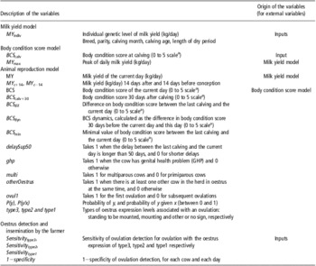
The developed animal reproduction model is a dynamic and stochastic simulation model, built as a succession of stochastic stages. As it is sensitive to MY and body condition score (BCS), this part describes the MY and BCS curves and then the reproduction model itself. Reproduction equations are detailed in a chronological manner, from resumption of ovarian activity after calving to the possible establishment of pregnancy and subsequent calving. All the variables used in the model are grouped in Table 1.
Variables used in the model

a0 is very thin; 5 is very fat.
Description of the MY and BCS curves
MY and BCS (on a 0 to 5 scale) variations were modelled with two curves, according to lactation stage. The MY curve was modelled using the French genetic test-day model, which mainly represents the effects of breed, parity, calving month, calving age, length of dry period, lactation stage and pregnancy stage on MY, using cubic spline curves (Leclerc et al., Reference Leclerc, Duclos, Barbat, Druet and Ducrocq2008). Thus, in our model, MY was calculated from the sum of the different effects of this genetic model, which generates the shape of the curve, plus an individual constant MY level, MY indiv, which depends on the production level of cow. The genetic model represents the lactation curve until 305 days in milk. This model was then linearly extrapolated to simulate longer lactations.
In accordance with the programmed energy mobilization in early lactation (Faverdin et al., Reference Faverdin, Delaby and Delagarde2007) that is genetically driven (Friggens et al., Reference Friggens, Brun-Lafleur, Faverdin, Sauvant and Martin2013), the equations that simulate BCS variations (INRA, 2010) were established using the database obtained by Delaby et al. (Reference Delaby, Faverdin, Michel, Disenhaus and Peyraud2009) on the same herd:
 $${BCS\: = \:BC{{S}_{{\rm{calv}}}}\:\times \:\left[ {a\: + \:b\:\times \:\exp \left( {{\rm{ - }}c\:\times \:W} \right) \: + \:d\:\times \:W} \right] $$
where BCS calv is BCS at calving, W is week of lactation, and for primiparous cows:
 $$ a\: = \:{\rm{1}}{\rm{.3}}\:{\rm{ - }}\:{\rm{0}}{\rm{.025}}\:\times \:M{{Y}_{\max }} $$
 $$ b\: = \:{\rm{ - 0}}{\rm{.3}}\: + \:{\rm{0}}{\rm{.025}}\:\times \:M{{Y}_{\max }} $$
 $$ c\: = \:{\rm{0}}{\rm{.24}} $$
 $$ d\: = \:{\rm{ - 0}}{\rm{.0062}}\: + \:{\rm{0}}{\rm{.00050}}\:\times \:M{{Y}_{\max }} $$
and for multiparous cows:
 $$ a\:= \:{\rm{1}}{\rm{.3}}\:{\rm{ - }}\:{\rm{0}}{\rm{.020}}\:\times \:M{{Y}_{\max }} $$
 $$ b\: = \:{\rm{ - 0}}{\rm{.3}}\: + \:{\rm{0}}{\rm{.020}}\:\times \:M{{Y}_{\max }} $$
 $$ c\: = \:{\rm{0}}{\rm{.24}} $$
 $$ d\: = \:{\rm{ - 0}}{\rm{.0045}}\: + \:{\rm{0}}{\rm{.00035}}\:\times \:M{{Y}_{\max }} $$
where MY max is the peak of daily MY. For primiparous cows, the equation was built (thanks to 1510 data), from 120 lactations, with MY max = 35.5 ± 3.14 kg and BCS calv = 3.5± 0.5 points, and had a residual standard error of 0.020. For multiparous cows, the equation was built (thanks to 1842 data), from 151 lactations, with MY max = 44.8 ± 4.04 kg and BCS calv = 2.85 ± 0.5 points, and had a residual standard error of 0.013.
Origin of the equations for the reproduction model
We chose to build the reproduction model from a unique source of data as far as possible. The data set used was from the study by Cutullic et al. (Reference Cutullic, Delaby, Gallard and Disenhaus2011). In short, their experiment was designed to produce strong variability in MY and BCS between cows fed at two contrasting feeding levels. The originality of this database lies in partial uncoupling between MY and BCS, which are highly negatively correlated in dairy cows similarly fed. This made it possible to differentiate MY effects from BCS effects on the different reproductive steps and to establish relationships between reproductive outcome and these two factors (Cutullic et al., Reference Cutullic, Delaby, Gallard and Disenhaus2012).
For reproductive steps where equations from these papers were unavailable or not directly usable in the model, we preferentially built equations based on the same database. Finally, if these sources were not usable, equations were added from other sources. Most of the time, our decision about which variable had to be included in the equations of our model for each process came from the statistical analysis of Cutullic et al. (Reference Cutullic, Delaby, Gallard and Disenhaus2012). For each rebuilt equation, the significance of the included variables was checked (no major change was found): the P-values of each included variable are provided in the text. For multinomial logistic regressions, the P-value of the decrease in the residual deviance, which is a measure of goodness of fit, is also given.
Genital health problems (GHP) at or following calving
The occurrence of GHP, that is, metritis, placental retention or vaginal infection, at or following calving was included in the model for its impact on the calving-to-first ovulation (CFO) interval. Although a decrease in BCS increases the risk of GHP (Friggens et al., Reference Friggens, Disenhaus and Petit2010), we applied a unique and fixed probability of GHP occurrence to every cow, equal to 0.28 for each calving. This value was the observed frequency of GHP in the original database (n = 98 lactations).
CFO interval
The CFO was estimated from calving to the commencement of luteal activity. It is longer for primiparous than for multiparous cows (Disenhaus et al., Reference Disenhaus, Cutullic, Blanc and Agabriel2009). GHP occurrence and low BCS in early lactation affect CFO (Opsomer et al., Reference Opsomer, Grohn, Hertl, Coryn, Deluyker and de Kruif2000; Roche et al., Reference Roche, Friggens, Kay, Fisher, Stafford and Berry2009). The choice was made to randomly draw CFO in a normal distribution around a mean value adjusted for the above factors instead of calculating it deterministically, in order to better represent the strong variability of CFO between cows. Cutullic et al. (Reference Cutullic, Delaby, Gallard and Disenhaus2012) showed that BCS 30 days after calving was the best predictive variable of commencement of luteal activity (C-LA), which occurs 4 days after ovulation, on average. In our model, in practice, CFO was determined thanks to C-LA and log-transformed to obtain a homoscedastic distribution per parity. The distribution of the mean of the natural logarithm of CFO plus 4 days (loge(CFO+4)) was fitted to the data with a linear regression (residual standard error: 0.46), including the effect of the parity ( $$$ P\: = \:{\rm{1}}{\rm{.31}}\:\times \:{\rm{1}}{{{\rm{0}}}^{{\rm{ - 3}}}} $$$
), GHP (
 $$$ P\: = \:{\rm{7}}{\rm{.48}}\:\times \:{\rm{1}}{{{\rm{0}}}^{{\rm{ - 3}}}} $$$
) and linear and quadratic effects of BCS 30 days after calving (
 $$$ P\: = \:{\rm{6}}{\rm{.18}}\:\times \:{\rm{1}}{{{\rm{0}}}^{{\rm{ - 5}}}} $$$
and
 $$$ P\: = \:{\rm{4}}{\rm{.57}}\:\times \:{\rm{1}}{{{\rm{0}}}^{{\rm{ - 4}}}} $$$
, respectively). The mean (μ) and s.d. (σ) of loge(CFO + 4) were described by the following equations:
 $$ no{ \mu \: = \:{\rm{4}}{\rm{.834}}\:{\rm{ - }}\:{\rm{0}}{\rm{.222}}\:\times \:multi\: + \:{\rm{0}}{\rm{.221}}\:\times \:ghp\:{\rm{ - }}\:{\rm{0}}{\rm{.939}}\:\cr \times \:BC{{S}_{{\rm{calv}}\:{\rm{ + }}\:{\rm{30}}}}\: + \:{\rm{0}}{\rm{.152}}\:\times \:BC{{S}_{{\rm{calv}}\:{\rm{ + }}\:{\rm{30}}}}^{{\rm{2}}} $$
 $$ \sigma \: = \:{\rm{0}}{\rm{.600}}\:{\rm{ - }}\:{\rm{0}}{\rm{.182}}\:\times \:multi $$
Oestrus expression
Oestrus detection is a crucial element of reproductive performance, which depends on both oestrus expression by the animal and its detection by the farmer. Both aspects were included in the model separately.
The level of oestrus expression is usually defined by its intensity, estimated by the nature and frequency of associated behavioural signs and by its duration (Kerbrat and Disenhaus, Reference Kerbrat and Disenhaus2004). For simplicity purposes, we chose to use only three levels of oestrus expression, on the basis of oestrus intensity: type 3 = ovulation associated with standing behaviour; type 2 = ovulation associated with mounting behaviour without standing; and type 1 = ovulation with only discreet oestrus expression (sniffing, licking, chin-resting, restless and clear mucous discharge) or without any behavioural signs. Equations were determined to calculate the probability of each of these three oestrus expression levels associated with an ovulation. The oestrus expression level is strongly increased by the concomitant presence of at least one other cow in oestrus (Kerbrat and Disenhaus, Reference Kerbrat and Disenhaus2004; Roelofs et al., Reference Roelofs, Lopez-Gatius, Hunter, van Eerdenburg and Hanzen2010). Expression is lower for first ovulation than subsequent ovulations. For subsequent ovulations, the oestrus expression is increased mainly by decreased MY around ovulation, and to a lesser extent by increased BCS (Lopez et al., Reference Lopez, Satter and Wiltbank2004; Cutullic et al., Reference Cutullic, Delaby, Gallard and Disenhaus2012). BCS, reflecting energy balance, could be the main risk factor at first ovulation (Berghorn et al., Reference Berghorn, Allrich and Noller1988) but this effect was yet insufficiently documented to be correctly modelled. Owing to the moderate importance of first ovulation (often too early to lead to an insemination), we assumed this simplification.
The oestrus detection method used in a study by Cutullic et al. (Reference Cutullic, Delaby, Gallard and Disenhaus2011) was strongly standardized. In line with previous works (Van Eerdenburg et al., Reference Van Eerdenburg, Loeffler and vanVliet1996; Kerbrat and Disenhaus, Reference Kerbrat and Disenhaus2004), we assumed that oestrus expression and detection were highly correlated in our database. Therefore, we adjusted oestrus detection data to estimate oestrus expression. Looking at the quality of the detection, we considered that 5% of type 3- and 5% of type 2-expressed ovulations were undetected. Remaining undetected ovulations were considered type 1 (L. Delaby and C. Disenhaus, personal communication). The probabilities of the three oestrus expression levels are given by the following equations for the first ovulation:
 $$ P\left( {type{\rm{3}}} \right)\: = \:{\rm{0}}{\rm{.027}}\: + \:{\rm{0}}{\rm{.211}}\:\times \:otherOestrus\: + \:{\rm{0}}{\rm{.05}} $$
 $$ P\left( {type{\rm{2}}} \right)\: = \:{\rm{0}}{\rm{.041}}\: + \:{\rm{0}}{\rm{.102}}\:\times \:otherOestrus\: + \:{\rm{0}}{\rm{.05}} $$
 $$ P(type{\rm{1}})\: = \:{\rm{1}}\:{\rm{ - }}\:P(type{\rm{2}})\:{\rm{ - }}\:P(type{\rm{3}}) $$
They are given by the following equations for subsequent ovulations:
 $$ P\left( {type{\rm{3}}} \right)\: = \:\frac{{\rm{1}}}{{{\rm{1}}\: + \:{{U}_{\rm{1}}}\: + \:{{U}_{\rm{2}}}}}\: + \:{\rm{0}}{\rm{.05}} $$
 $$ P\left( {type{\rm{2}}} \right)\: = \:\frac{{{{U}_{\rm{1}}}}}{{{\rm{1}}\: + \:{{U}_{\rm{1}}}\: + \:{{U}_{\rm{2}}}}}\: + \:{\rm{0}}{\rm{.05}} $$
 $$ P\left( {type{\rm{1}}} \right)\: = \:\frac{{{{U}_{\rm{2}}}}}{{{\rm{1}}\: + \:{{U}_{\rm{1}}}\: + \:{{U}_{\rm{2}}}}}\:{\rm{ - }}\:{\rm{0}}{\rm{.10}} $$
where
 $$ \displaylines{ {{U}_{\rm{1}}}\: = & \:\exp ({\rm{ - 2}}{\rm{.866}}\:{\rm{ - }}\:{\rm{0}}{\rm{.264}}\:\times \:otherOestrus\: + \:{\rm{0}}{\rm{.0422}}\: \cr & \times \:MY\: + \:{\rm{0}}{\rm{.338}}\:\times \:BCS) $$
and
 $$ \displaylines{ {{U}_{\rm{2}}}\: = & \:\exp ({\rm{ - 1}}{\rm{.097}}\:{\rm{ - }}\:{\rm{1}}{\rm{.081}}\:\times \:otherOestrus\: + \:{\rm{0}}{\rm{.0832}}\: \cr & \times \:MY\:{\rm{ - }}\:{\rm{0}}{\rm{.557}}\:\times \:BCS) $$
The parameters of these equations were readjusted on the original database. For the first ovulations (n = 95), these equations were directly built from the observed frequency of the three types of oestrus. For the subsequent ovulations (n = 219), the parameters of the equations were adjusted with a multinomial logistic regression (decrease in the residual deviance:  $$$ P\: = \:{\rm{3}}{\rm{.56}}\:\times \:{\rm{1}}{{{\rm{0}}}^{{\rm{ - 6}}}} $$$
), including the effect of having another cow in ovulation on the same day v. not (otherOestrus,
 $$$ P\: = \:{\rm{2}}{\rm{.51}}\:\times \:{\rm{1}}{{{\rm{0}}}^{{\rm{ - 3}}}} $$$
), MY (
 $$$ P\: = \:{\rm{2}}{\rm{.50}}\:\times \:{\rm{1}}{{{\rm{0}}}^{{\rm{ - 4}}}} $$$
) and BCS (
 $$$ P\: = \:{\rm{1}}{\rm{.58}}\:\times \:{\rm{1}}{{{\rm{0}}}^{{\rm{ - 2}}}} $$$
) on the day of the ovulation.
Oestrus detection and insemination
Oestrus detection and insemination were not a part of the animal reproduction model stricto sensu, as it represented the management by the farmer. However, inseminations had to be modelled. We considered that each oestrus that could be detected would conduct to systematic mating. Oestrus detection depends on the oestrus expression by the cow and on the detection performance of the farmer. It is modelled by a set of four probabilities: three probabilities of ovulation detection, one for each of type 1-, type 2- and type 3-expressed ovulations (representing the sensitivity of oestrus detection), and one probability of concluding that a cow is in oestrus, whereas it has not ovulated (=1 minus the specificity of oestrus detection).
Cycle length
Cycle length was mainly determined by cycle type: normal, short or with a PLP. Cutullic et al. (Reference Cutullic, Delaby, Gallard and Disenhaus2012) showed that the probability of occurrence of these different types depends on BCS variations. Indeed, the probability of having a PLP is high when ovulation occurs while BCS is strongly decreasing. Conversely, the probability of having a short cycle is high when BCS is not decreasing anymore or even increasing, all the more when BCS has previously deeply decreased from calving to ovulation. Cutullic et al. (Reference Cutullic, Delaby, Gallard and Disenhaus2012) used the body condition slope from −30 to +30 d relative to the day of ovulation in their model. This variable cannot be directly included in our model because the cycle type must be determined on the day of the ovulation to plan the next one and the value of BCS at 30 days later is still unknown. Instead, we used BCS dyn, calculated as the difference in BCS between 30 days before the ovulation and the day of this ovulation. As the first cycle differs strongly from subsequent cycles (high probability of short cycles), predictive equations for cycle type include the effect of first v. subsequent cycles. Finally, the equations included in our model to predict the probabilities of the different cycle types are equations 20 to 24:
 $$ P(normalCycle)\: = \:\frac{{\rm{1}}}{{{\rm{1}}\: + \:{{V}_{\rm{1}}}\: + \:{{V}_{\rm{2}}}}} $$
 $$ P\left( {shortCycle} \right)\: = \:\frac{{{{V}_{\rm{1}}}}}{{{\rm{1}}\: + \:{{V}_{\rm{1}}}\: + \:{{V}_{\rm{2}}}}} $$
 $$ P\left( {PLP} \right)\: = \:\frac{{{{V}_{\rm{2}}}}}{{{\rm{1}}\: + \:{{V}_{\rm{1}}}\: + \:{{V}_{\rm{2}}}}} $$
where
 $$ \displaylines{ {{V}_{\rm{1}}}\: = & \:\exp ({\rm{ - 5}}{\rm{.298}}\: + \:{\rm{4}}{\rm{.763}}\:\times \:ovul{\rm{1}}\: + \:{\rm{2}}{\rm{.669}} \cr & \:\times \:BC{{S}_{{\rm{dyn}}}}\:{\rm{ - }}\:{\rm{1}}{\rm{.863}}\:\times \:BC{{S}_{{\rm{dif}}}}) $$
and
 $$ \displaylines{ {{V}_{\rm{2}}}\: = & \:\exp ({\rm{ - 2}}{\rm{.461}}\: + \:{\rm{0}}{\rm{.474}}\:\times \:ovul{\rm{1}}\:{\rm{ - }}\:{\rm{1}}{\rm{.422}}\:\times \:BC{{S}_{{\rm{dyn}}}}\: \cr & + \:{\rm{0}}{\rm{.306}}\:\times \:BC{{S}_{{\rm{dif}}}}) $$
These equations were readjusted on the original database (n = 189 short cycles, normal cycles or PLP) with a multinomial logistic regression (decrease in the residual deviance:  $$$ P\: = \:{\rm{5}}{\rm{.76}}\:\times \:{\rm{1}}{{{\rm{0}}}^{{\rm{ - 3}}}} $$$
), including the effect of first v. subsequent cycles (
 $$$ P\: = \:{\rm{1}}{\rm{.40}}\:\times \:{\rm{1}}{{{\rm{0}}}^{{\rm{ - 11}}}} $$$
), BCS dyn (
 $$$ P\: = \:{\rm{1}}{\rm{.25}}\:\times \:{\rm{1}}{{{\rm{0}}}^{{\rm{ - 5}}}} $$$
) and BCS difference between the calving and this ovulation (BCS dif,
 $$$ P\: = \:{\rm{1}}{\rm{.66}}\:\times \:{\rm{1}}{{{\rm{0}}}^{{\rm{ - 3}}}} $$$
).
The cycle length distribution law for each cycle type was also derived from the original database. For short and normal cycles, the cycle length follows normal distributions, with mean of 22.75 and 10.70 days, respectively, and s.d. of 3.17 and 1.66 days, respectively. These parameters were estimated from the database (estimated s.e.m.: 0.31 days for short cycles (n = 27) and 0.27 days for normal cycles (n = 142)). For PLP, the ovulation–ovulation interval follows an exponential distribution of parameter 0.0307. This distribution was adjusted to the data (n = 26; estimated standard error of the rate: 0.00695).
Conception
The definitions of all the events following insemination are adapted from the studies by Humblot (Reference Humblot2001) and Santos et al. (Reference Santos, Thatcher, Chebel, Cerri and Galvão2004), and these events are determined from progesterone profiles and ultrasonography as described by Cutullic et al. (Reference Cutullic, Delaby, Gallard and Disenhaus2011). As non-fertilization and early embryo mortality (EEM) remain undistinguishable (Humblot, Reference Humblot2001), the model integrated them together as non-conception.
The probability of conception at a given insemination is influenced by the level of body reserves (Roche et al., Reference Roche, Friggens, Kay, Fisher, Stafford and Berry2009). Cutullic et al. (Reference Cutullic, Delaby, Gallard and Disenhaus2012) showed that the level of BCS at nadir affected this probability. To estimate the probability of conception, our model can only use present or past values of BCS, and hence we chose to use the minimal value of BCS between calving and insemination (BCS min). Consistently with uterine involution delay (Inchaisri et al., Reference Inchaisri, Hogeveen, Vos, van der Weijden and Jorritsma2010b), the model included the impact of insemination before or after 50 days post calving. In our model, the probability of conception for each insemination is given by the following equations:
 $$ P\left( {conception} \right)\: = \:\frac{U}{{{\rm{1}}\: + \:U}}\:\times \:{{k}_{\rm{1}}} $$
where
 $$ no{ U\: = & \:\exp ({\rm{ - 2}}{\rm{.06}}{{{\rm{4}}}^{\rm{f}}} \: + \:{\rm{0}}{\rm{.696}}\:\times \:BC{{S}_{\min }}\: + \:{\rm{1}}{\rm{.386}}\: \cr & \times \:delaySup{\rm{50}}) \ \ \ \ \ \ \ \ \ \ \ \ \ \ \ \ \ \ \ \ \ \ \ \ \ \ \ \ \ \ \ \ \ \ \ \ (26) $$
and
 $${{k}_{\rm{1}}}\: = \:{\rm{1}}\:{\rm{ - }}\:{\rm{0}}{\rm{.02}}\:\times \:\left( {MY_{\rm indiv}\:{\rm{ - }}\:{\rm{30}}} \right)$$
These equations were first adjusted on the original database with a binomial logistic regression (n = 128 inseminations; decrease in the residual deviance:  $$$ P\: = \:{\rm{9}}{\rm{.89}}\:\times \:{\rm{1}}{{{\rm{0}}}^{{\rm{ - 3}}}} $$$
), including the effect of BCS min (
 $$$ P\: = \:{\rm{2}}{\rm{.36}}\:\times \:{\rm{1}}{{{\rm{0}}}^{{\rm{ - 2}}}} $$$
) and the delay between calving and insemination (<50 v. ≥50;
 $$$ P\: = \:{\rm{1}}{\rm{.43}}\:\times \:{\rm{1}}{{{\rm{0}}}^{{\rm{ - 2}}}} $$$
). Then, as we also know that this probability of conception is influenced by the genetically driven MY potential of the cow, an effect of MY indiv was estimated from the study by Grimard et al. (Reference Grimard, Fréret, Chevallier, Pinto, Ponsart and Humblot2006) and included in the model.
Embryo survival
After conception, pregnancy can be ended by late embryo mortality (LEM, inducing a fall in progesterone within 50 days post insemination) or later by foetal mortality or abortion (grouped together under the term ‘abortion’). Frequency of LEM increases with peak MY, and the shape of the lactation curve is thought to affect embryo survival, with sharp curves having negative effects (Grimard et al., Reference Grimard, Fréret, Chevallier, Pinto, Ponsart and Humblot2006). As suggested by Cutullic et al. (Reference Cutullic, Delaby, Gallard and Disenhaus2012), an effect of MY slope around conception accounts for this effect in the model, with the probability of LEM being described by the following equations:
 $$ P\left( {LEM\:/\:conception} \right)\: = \:\frac{V}{{{\rm{1}}\: + \:V}} $$
where
 $$ V\: = \:\exp\! \left( {{\rm{ - 1}}{\rm{.343}}{{{\rm{8}}}^{\rm{g}}} \:{\rm{ - }}\:{\rm{5}}{\rm{.7696}}\:\times \:\frac{{M{{Y}_{c\: + \:{\rm{14}}}}\:{\rm{ - }}\:M{{Y}_{c\:{\rm{ - }}\:{\rm{14}}}}}}{{{\rm{28}}}}} \right) $$
The parameters of this model were adjusted on the original database (n = 78 conceptions) with a binomial logistic regression ( $$$ P\: = \:{\rm{2}}{\rm{.41}}\:\times \:{\rm{1}}{{{\rm{0}}}^{{\rm{ - 3}}}} $$$
).
None of the BCS variables (levels, slopes and changes at various stages of lactation) had any effect on the frequency of LEM (Cutullic et al., Reference Cutullic, Delaby, Gallard and Disenhaus2012). Conversely, many variables concerning MY around the lactation peak affected this frequency (Cutullic et al., Reference Cutullic, Delaby, Gallard and Disenhaus2012). The probability of abortion when embryo is not affected by LEM (and therefore it survives at least until 50 days) was set to 0.03.
After LEM, the ovulation–ovulation interval was drawn in a uniform distribution between 25 and 50 days, and after an abortion it is drawn in a uniform distribution between 50 and 250 days.
Implementation of the reproduction model
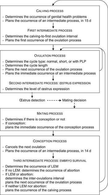
The computer model is dynamic and daily time stepped. The reproduction process is viewed as a succession of discrete processes. Figure 1 illustrates the model processes and their main actions. All the processes are registered in an agenda and the time progresses from one process to the other, following in chronological order. Nothing happens between two successive processes. The principle of the model is that each reproductive step is represented by a unique discrete process that plans the following one in the agenda (e.g. the calving plans the first ovulation; each ovulation plans the following one…). The progression of a cow from one reproductive state to another one is mainly represented by a few descriptors attached to each cow. The ‘fertilizable’ descriptor is switched from 0 to 1 by the ovulation process and switched back to 0 one day after. The ‘pregnant’ descriptor is switched from 0 to 1 by the conception process and switched back to 0 in case of calving or pregnancy interruption (LEM or abortion). The level of oestrus expression is also recorded. These descriptors are completed by the recording of the last date and number of the calving and ovulation processes.
Representation of the cow reproduction computer model with the main actions of the six successive discrete processes. Solid arrows represent the planning of the occurrence of a discrete process, whereas dashed arrows represent farmer interventions. PLP = prolonged luteal phase; LEM = late embryonic mortality.

For practical reasons, calving, ovulation and conception processes are represented by more than one process (Figure 1). In these cases, the model includes intermediate processes. The first and third intermediate processes were inserted because the calving and conception processes needed values of MY or BCS that were not already known to plan the following processes. The second intermediate process was inserted to take into account an interaction between cows for oestrus expression.
In more detail, the calving process needed BCS at 30 days after calving (BCS calv+30) to calculate the CFO and then plan the first ovulation in the agenda. Therefore, the calving process was split into two successive steps: the calving process stricto sensu and the first intermediate process, 15 days after calving, whose function is only to calculate the CFO and plan the first ovulation. This intermediate process could not be planned at 30 days post calving, because many first ovulations occurred before this delay (56%, n = 98). Consequently, we chose to estimate BCS calv+30 by linear extrapolation of BCS variation between calving and 15 days after. This modelling option implies that no simulated CFO will be shorter than 15 days, which appears an acceptable approximation.
The conception process needed MY at 14 days post conception to calculate the probability of LEM, and then plan the process following conception (calving or ovulation) in the agenda. Hence, the conception process was split into two successive steps: the conception process stricto sensu and the third intermediate process, 14 days after conception, whose function is to calculate the probabilities of LEM and abortion, and to plan the process following conception in the agenda.
Finally, the second intermediate process was inserted after the ovulation process but in the same time step to determine the degree of oestrus expression. Indeed, the oestrus expression of one cow is dependent on whether at least one other cow is in oestrus at the same time, which the model assumes as equating to the fact that at least one other cow is ovulating at the same time. Therefore, before the oestrus expression can be determined for one cow, a process has to already know whether the other cows ovulated. This prompted us to split the ovulation process into two successive steps, the first step being ovulation stricto sensu, and the second step being the determination of the level of the oestrus expression.
Many steps of the reproduction model are stochastic. Indeed, several processes can lead to different possible outcomes. In this case, in practice, when a reproductive step can lead to N possible different outcomes, the process proceeds in two stages: first, it calculates the occurrence probability Pk of each outcome k ( $$$ \sum _{{k\: = \:{\rm{1}}}}^{N} {{P}_k}\: = \:{\rm{1}} $$$
); second, it draws x in a uniform distribution between 0 and 1, and finally concludes that the outcome is the first one if x < P 1 and outcome i, with i > 1, if
 $$$ \mathop{\sum}\nolimits_{k\: = \:{\rm{1}}}^{i\:{\rm{ - }}\:{\rm{1}}} {{{P}_k}} \:\leq \:x\: \less \:\mathop{\sum}\nolimits_{k\: = \:{\rm{1}}}^i {{{P}_k}} $$$
.
Description of the simulations
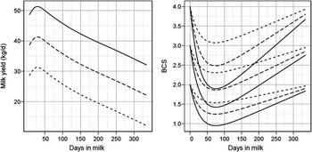
To test the sensitivity of the model to MY and BCS, we used a complete factorial sampling design with three levels of individual genetic MY, MY indiv and three levels of BCS at calving, BCS calv. MY indiv varied in the set {25; 35; 45} (Figure 2). This range of variation corresponded to a cow that produced about 6700 kg to 12 900 kg of milk in 305 days. BCS calv varied in the set {2; 3; 4}.
Milk yield (left) and body condition score (BCS, 0-5 scale, right) curves used to test the sensitivity of the reproduction model to individual milk yield level (MY indiv, kg) and BCS at calving. These curves correspond to three values of MY indiv, that is, 25 kg (dashed), 35 kg (long-dash) and 45 kg (solid), and three values of BCS at calving: 2, 3 and 4. The decreasing effect of pregnancy on milk yield is not charted in this figure.

All the simulations were run with identical cows, that is, Holsteins calving in November for their third calving at 50 months old after being dried off 60 days before calving. Each set of parameters was tested via 20 simulations. Each simulation was run on a group of 50 cows. Using the groups of cows enabled to take into account the interaction between the cows, which increases oestrus expression in real groups of cows compared with the oestrus expression for separated cows. The first day of the simulations was the calving date of the cows.
To test the individual animal reproduction model, we chose to limit the restraints linked to management decisions. Therefore, reproduction management was favourable to successful reproduction, with relatively high levels of oestrus detection sensitivity and specificity and a long reproduction period. In fact, each day each ovulating cow was given a probability of being inseminated of 0.20 for the expression of type 1, 0.80 for the expression of type 2 and 0.90 for the expression of type 3, whereas each cow that did not ovulate had a probability of being inseminated of 0.0002. Moreover, the simulations were run over 600 days, which enabled us to evaluate all the reproductive stages during a complete calving-to-calving interval. Cows could be mated from 50 days post calving to the end of the simulation. In order not to interfere with the test of the reproduction model, we did not include any culling decision during these simulations.
Studied outputs and statistical analysis
We first chose to study overall recalving rate (%) and calving interval (CI, days), as they are aggregated variables representing overall success of reproduction in a herd in terms of rate of success and reproduction delays (there was no culling in the simulations). However, without any limit on the reproduction period, almost all of the cows would end up recalving, thus increasing recalving rate to almost 100%, while also increasing CI. Therefore, we also studied these two outputs for a limited reproduction period of 90 days for each cow (from 50 to 140 days after calving) and the cumulative proportion of pregnant cows according to the days after calving. These simulation results were analysed with the following model:
 $$ \displaylines{ {{Y}_{\rm{i}}}\: = & \:\mu \: + \:{{k}_{\rm{M}}}\:\times \:M{{Y}_{{\rm{indiv}}}}\: + \:{{k}_{\rm{B}}}\:\times \:BC{{S}_{{\rm{calv}}}}\: + \:{{k}_{{\rm{MB}}}}\: \cr & \times \:M{{Y}_{{\rm{indiv}}}}\:\times \:BC{{S}_{{\rm{calv}}}}\: + \:{{e}_i} $$
where Yi is the studied model output for simulation i, μ is the mean, k M, k B and k MB are the effects of MY indiv, BCS calv and their interaction and ei is the error associated with each Yi. When these effects were not significant (P > 0.05), the model was simplified with only additive effects, or even with only the MY indiv effect or the BCS calv effect.
Results
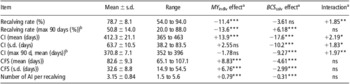
The reproduction model, composed of an aggregation of equations coming from the successive reproductive steps, succeeded in simulating consistent overall reproductive performance (Table 2).
Results of the sensitivity analysis to MY indiv and BCS calv (equation (30)): effect of a MY indiv (expressed per 10 kg of milk) and BCS calv (expressed per point, 0 to 5 scale) on the main reproduction outputs of the model, plus mean, s.d. and range of these outputs. Mean, s.d. and range were calculated from the average values per simulation (n = 160)

CI = calving interval; CFS = calving-to-first service interval; AI = artificial inseminations.
a***, **, * = significant effect with P < 0.001, P < 0.01 and P < 0.05; ns = non-significant effect (P ⩾ 0.05).
bmax 90 d = if the reproduction period length were limited to 90 days for each cow.
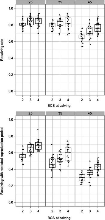
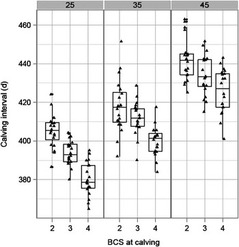
The reproduction results, including recalving rate and CI as the most aggregated variables, were sensitive to both MY indiv and BCS calv (Table 2, Figures 3–5). Overall, the results indicate that an increase in MY indiv or a decrease in BCS calv penalized reproduction, decreasing the recalving rate for the short reproduction period by about 14 points per 10 kg of milk and six points per BCS point (Figure 3), and increasing the CIs by about 20 days/10 kg of milk and 10 days/BCS point (Figures 4 and 5).
Average recalving rate (top) and average recalving rate for cows whose reproduction period is capped at 90 days (bottom) according to MY indiv (kg, column facets) and to body condition score (BCS) at calving (x-axis). Each point represents the average value for one simulation. Boxes represent the median and quartiles of the distribution of these points for each parameter set.

Average calving interval according to MY indiv (kg, column facets) and to body condition score (BCS) at calving (0 to 5 scale, x-axis). Each point represents the average value for one simulation. Boxes represent the median and quartiles of the distribution of these points for each parameter set.

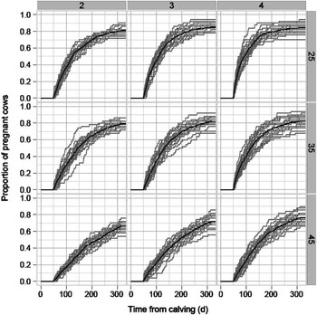
Cumulative proportion of pregnant cows according to individual milk yield level (MY indiv, kg, rows) and body condition score (BCS) at calving (columns). Grey lines correspond to individual simulations and black lines correspond to the average curve per treatment.

The observed interactions between MY indiv and BCS calv on recalving rate for the long reproduction period and on CI for the short reproduction period resulted from a saturation phenomenon: for the long reproduction period, an improved reproductive performance mainly led to a shortening of CI as recalving rate got nearer the ceiling of 1, and for the short reproduction period, the decline in reproductive performance mainly resulted in a decrease in recalving rate because the CI was capped.
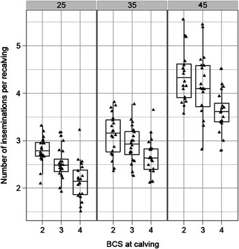
Focusing on less-aggregated reproduction variables, an increased MY indiv or a decreased BCS calv increased the reproduction delays. It increased the average calving-to-first service interval (CFS, days) by about 9 days/10 extra kg of milk and 4 days/BCS point less (Figure 6), by decreasing the oestrus expression for MY indiv and increasing CFO for BCS calv. Moreover, it also decreased conception rate and consequently increased calving to conception interval. By penalizing insemination success, the number of inseminations per recalving (total number of inseminations divided by total number of calvings in the cow group) also increased by about 0.5 AI for 6.3 extra kg of milk or for 1.6 point of BCS at calving less (Figure 7).
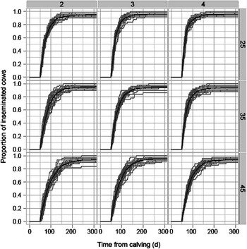
Cumulative proportion of inseminated cows according to individual milk yield level (MY indiv, kg, rows) and body condition score at calving (columns). Grey lines correspond to individual simulations and black lines correspond to the average curve per treatment.

Number of inseminations in the group of cows per obtained recalving obtained over the entire reproduction period, according to MY indiv (column facets) and body condition score (BCS) at calving (x-axis). Each point represents the average value for one simulation. The boxes represent the median and quartiles of the distribution of these points for each parameter set.

Sensitivity analysis also showed high between-simulations variability in reproductive performance (Figures 5 and 6). Indeed, for the same parameter set, between the worst and the best simulation, recalving rate for the short reproduction period ranged from 16 to 40 points according to the parameter set, and CI for the long reproduction period ranged from 24 to 60 days. There was also a broad variability between identical cows. Moreover, this variability increased with increasing MY and decreased with increasing BCS at calving, as shown by analysis of the s.d. on CI and CFS in Table 2.
Discussion
Choice of the equations of the model
We are aware that the individual energy balance of cows may have been a more accurate risk factor than BCS change variables for some reproductive stages; however, this information was not available in the experiment of Cutullic et al. (Reference Cutullic, Delaby, Gallard and Disenhaus2011). BCS also has the advantage of being more directly measurable than energy balance, and to be interpretable as both level and change. For these reasons, the present model only relies on BCS.
We chose to use a unique database, as it made possible to build equations for almost all reproductive stages for the same cows in the same conditions, thus guaranteeing the coherence of the model. This option raises the question of the genericity of the model to represent cows from other herds; however, as previously said, the experimental design generated a large variability in both MY and BCS. Obtaining equations from different sources would not solve this problem, if each reproductive stage equation was built from one source. Meta-analysis was considered, but with the exception of calving to commencement of luteal activity, few literature sources were available with the level of details we needed and homogeneous definitions for reproductive parameters, as well as for MY and BCS variables. Moreover, using BCS data in a meta-analysis is very difficult, owing to the use of different non-proportional scales (Roche et al., Reference Roche, Dillon, Stockdale, Baumgard and VanBaale2004) and to the frequent need to finally simplify it as a two to three categories variable (Lopez-Gatius et al., Reference Lopez-Gatius, Yaniz and Madriles-Helm2003). In the database, there were two experimental groups (high v. low feeding level), which can also be a limit of the model, in a statistical point of view.
The partial uncoupling between MY and BCS in our database, owing to the use of two contrasting feeding strategies, was very useful to distinguish the proper effects of MY from the effects of BCS. In common herds, MY and BCS changes are strongly correlated, so that both effects may act together, and the estimated effects of either MY or BCS would be exaggerated. Conversely, our model should be able to simulate plausible reproduction results in a wide range of situations: globally, a low-MY/high-BCS case will lead to a better reproductive performance than in a low-MY/low-BCS or high-MY/high-BCS case, in turn better than in a high-MY/low-BCS case.
Concerning oestrus expression, the between-cows interaction in terms of oestrus expression may be overestimated in our simulations because all cows calve on the same day at the beginning of the simulation, and thus are more synchronized than in most of the real herd. However, the variability of CFO interval and cycle length rapidly decreases this synchronization bias all the more, as cows could not be mated before 50 days after calving.
Comparison of simulation outputs against data from the original database
Our model was built as a succession of numerous reproductive steps. Therefore, it appeared important to first compare the aggregated simulated reproductive performance, recalving rate and CI, with the actual performances observed in the data of from the study by Cutullic et al. (Reference Cutullic, Delaby, Gallard and Disenhaus2011 and Reference Cutullic, Delaby, Gallard and Disenhaus2012). Indeed, the equations of each reproductive step had their own errors. Even if these errors were small, they could create non-negligible errors at the scale of a calving-to-calving reproductive cycle through error accumulation. As this database corresponded to cows managed under a 13-week reproduction period, we considered the recalving rate simulated for the short reproduction period and compared it with the observed rate for multiparous Holstein cows fed at a high feeding level (n = 30). CI is not a meaningful indicator for such a management and therefore was not considered. The cows of the database had a BCS calv of 2.86 (s.d. 0.46), a maximum MY of 45.0 kg (s.d. 5.4 kg), and a total MY produced in 305 days of about 9000 kg (s.d. 1100 kg). Thus, they were compared with the closest simulations in terms of MY and BCS, that is, simulations from the analysis of sensitivity to MY and BCS with a MY indiv of 35 kg and a BCS calv of 3.0. The database recalving rate was 50%, whereas the corresponding simulated recalving rate averaged 53% (s.d. 7.1), ranging from 38% to 64%, depending on the simulation. For the cows in the database, abortion rate, given successful conception and no LEM was 7% v. 3% in the simulations. This difference could result in a one- to two-point drop in recalving rate. In conclusion, the model was able to satisfactorily represent the recalving rate observed in the database.
Comparison of simulation outputs against reproductive performance in working farms
In commercial Holstein farms in France, CI averaged 408 days in 2006 and is increasing by about 1 day/year (Barbat et al., Reference Barbat, Druet, Bonaiti, Guillaume, Colleau and Boichard2005 and Reference Barbat, Le Mezec, Ducrocq, Mattalia, Fritz, Boichard, Ponsart and Humblot2010). The simulated CI in the analysis of sensitivity to MY and BCS averaged 412 days when all simulations were pooled and 410 days for the simulations involving medium-producing cows. The simulation results were therefore consistent with results recorded in working commercial farms. On one hand, our simulations may be optimistic, as they were realized with a high level of oestrus detection (our aim was to test the reproduction model aside from management effects). This is confirmed by the consistency between the simulated CFS, that averaged 83 days, and the average CFS of 88 days observed in Holstein cows in France (Barbat et al., Reference Barbat, Le Mezec, Ducrocq, Mattalia, Fritz, Boichard, Ponsart and Humblot2010). On the other hand, we allowed for a quite unrealistic CI of up to 600 days in simulations. Capping CI to a maximum of 550 days, for example, would result in a shorter CI average: 404 days for all simulations pooled and 402 days for the medium-producing cows. The modelled sensitivity of CI to MY level (about 20 days/10 kg of milk) is also comparable with the trend observed in French herds. Indeed, each year, CI increases by about 1 day and genetic potential by about 0.5 kg of peak MY (Pflimlin et al., Reference Pflimlin, Faverdin and Béranger2009).
The simulated CIs of our model are also globally consistent with the literature data on average but also in terms of sensitivity to MY level. Indeed, Petersson et al. (Reference Petersson, Strandberg, Gustafsson and Berglund2006) showed an increase in the calving-to-first oestrous interval of 0.89 days and in the first-to-last insemination of 0.63 days for an increase in MY of 1 kg during the first 60 days of lactation. This corresponds to an increase of about 15 days of CI per 10 kg of milk. Their results are close to those of the results observed by McGowan et al. (Reference McGowan, Veerkamp and Anderson1996) that obtained an increase in the calving-to-last insemination of about 16 days/10 kg of milk. These two results showed a lower effect of MY on the CI than our simulations (about 20 days of CI per 10 kg of milk), but the differences in MY were observed during the first 60 days of lactation for Petersson et al. (Reference Petersson, Strandberg, Gustafsson and Berglund2006) and the first 182 days of lactation for McGowan et al. (Reference McGowan, Veerkamp and Anderson1996), whereas the differences studied in our simulations concerned the whole 305 days lactation. Mackey et al. (Reference Mackey, Gordon, McCoy, Verner and Mayne2007) showed a higher effect of MY on the CI, with a difference in CI of 7.8 days/1000 kg increase in 305 days lactation, which correspond to an increase of about 24 days/10 kg of MY.
The simulated proportion of pregnant cows according to the lactation stage is also consistent with bibliography data for other European herds. Indeed, for cows with MY and BCS profiles similar to the simulations with a MY indiv of 35 kg and a BCS calv of 3, Suriyasathaporn et al. (Reference Suriyasathaporn, Nielen, Dieleman, Brand, Noordhuizen-Stassen and Schukken1998) obtained 50% of pregnant cows at 125 days post calving (n = 1404 lactations), whereas Mackey et al. (Reference Mackey, Gordon, McCoy, Verner and Mayne2007) obtained 45% at 118 days post calving (n = 2500 lactations), which is close to our simulated figures (Figure 5) of 44.5% of pregnant cows at 120 days post calving and 50% at 132 days post calving. However, the cumulative proportion of inseminated cows simulated by our model increased more rapidly than in the observation by Suriyasathaporn et al. (Reference Suriyasathaporn, Nielen, Dieleman, Brand, Noordhuizen-Stassen and Schukken1998), who reached a 50% rate of inseminated cows at 95 days post calving, whereas in our simulations the insemination rate reached 50% already by 73 days post calving and 73% by 95 days. This could be because of the particularly efficient oestrus detection in our simulations and to the fact that the model was built from the data on cows managed for a short reproduction period.
This model would merit further validation through a comparison of the simulated and observed reproductive performance. It would especially require other experimental data with detailed reproductive performance, and complete MY and BCS measurements. Forthcoming data from the same experimental herd should help in the future to improve the precision of the present model (e.g. health status) and maybe to add new equations to let aside stages (e.g. first ovulations, distinction between non-fertilization and early embryonic death). Although much more complicated and requiring much more cows, attention should also be paid in the future to the distinction between the genetic and the environment parts of the MY and BCS effects (e.g. genetic drive of cyclicity, of embryonic death). A first approach would be to adapt this model to other breeds such as the Normande or Montbéliarde. This first evaluation showed that our model was able to well simulate the overall reproductive performance observed in commercial Holstein farms in terms of both success rate and reproduction delays.
This model could be used to predict the demography of the herd (i.e. the parity composition and the lactation stages) in response to management strategies. As lactation stage represents a main factor of the MY dynamic and level, in turn the model could be used in a herd model to predict the forthcoming herd milk production and its uncertainty.
Conclusions
Despite being an aggregation of equations representing the successive steps of the reproductive process, the reproduction model succeeded in predicting consistent overall animal reproductive performance. It is sensitive to MY and body reserves, represented by BCS, and can thus be used to simulate demography in response to management decisions in a herd model.
Acknowledgements
The authors thank all the staff of the INRA Borculo farm at Le Pin-au-Haras for their cooperation in the management of the 5-year experiment and for carrying out the associated measurements. They also acknowledge Auvergne Traduction Technique (Clermont-Ferrand, France) for the revision of the English language.