2. Grid of photoionization models

Photoionization models require an ionizing spectrum as input radiation field. For this, we use stellar population synthesis models from pyStarburst99 (Hawcroft et al. Reference Hawcroft2025). The Starburst99 (Leitherer et al. Reference Leitherer1999) stellar population synthesis package was recently updated to pyStarburst99, incorporating the capability of generating models with stellar rotation, VMS and population III stars, among many other improvements. We consider the GENEC suite of stellar evolutionary tracks for metallicities $Z= 0, 0.0004, 0.002, 0.006, 0.014\ [Z_\odot]$ (Murphy et al. Reference Murphy2021; Groh et al. Reference Groh2019; Georgy et al. Reference Georgy2013; Eggenberger et al. Reference Eggenberger2021; Ekström et al. Reference Ekström2012). We make use of the stellar tracks with and without stellar rotation. Tracks with rotation assume an initial velocity of 40% of the equatorial break-up velocity. Models with $Z=10^{-5}$ (Ziegler et al. Reference Ziegler, Freese, Lozano and Montefalcone2025) and 0.020 (Yusof et al. Reference Yusof2022) will also be calculated and included for the final release of the grid. The stellar initial mass function of Kroupa (Reference Kroupa2001) with an upper limit (M $_\mathrm{up}$ ) of 120 $M_\odot$ is considered. Models with VMS were also calculated for $Z=0, 0.006$ and 0.014, where tracks with M $_\mathrm{up}=300~M_\odot$ are available. pyStarburst99 considers populations of single stars. These models were calculated with timesteps of 0.1 Myr up to 10 Myr. This upper age was selected as close binary interactions are expected to have significant effects on the ionizing radiation of a population at later times (Lecroq et al. Reference Lecroq2024).

We calculated the photoionization models with Cloudy version C23.02 (Ferland et al. Reference Ferland, Korista, Verner, Ferguson, Kingdon and Verner1998; Gunasekera et al. Reference Gunasekera, van Hoof, Chatzikos and Ferland2023). We consider two limiting cases for the hydrogen density, volume filling factor, geometry and dust content. The mean ionization parameter takes values of $\log(U) =-4, -3,-2$ . In order to be consistent with the population synthesis models, the ISM abundances are linearly scaled from the solar abundances of Asplund et al. (Reference Asplund, Grevesse, Sauval and Scott2009). N and C abundances are known to follow non-linear relations with respect to metallicity, as they present secondary nucleosynthetic production at high metallicities. We scale N/O and C/O according to the relations derived by Byler et al. (Reference Byler, Dalcanton, Conroy, Johnson, Levesque and Berg2018), also considering models that deviate from these by a factor of $\pm0.5$ dex. In total, we calculated 760 320 photoionization models. This number will increase once the $Z=10^{-5}$ and 0.020 models are included.

3. Comparison with observations and models of the literature

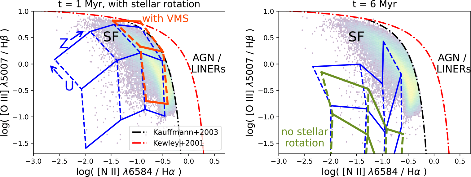
The BPT diagnostic diagram, described in Baldwin et al. (Reference Baldwin, Phillips and Terlevich1981), has been traditionally used to classify the principal source of ionizing photons in unresolved galaxies. The theoretical and empirical lines of Kewley et al. (Reference Kewley, Dopita, Sutherland, Heisler and Trevena2001) and Kauffmann et al. (Reference Kauffmann2003), respectively, delimit the region of galaxies dominated by ionization from star-forming regions (SF) instead of the narrow line regions of an active galactic nucleus (AGN). Figure 1 depicts the Kewley et al. (Reference Kewley, Dopita, Sutherland, Heisler and Trevena2001) and Kauffmann et al. (Reference Kauffmann2003) lines on the BPT diagram, as well as the sample of SF-dominated galaxies of SDSS-DR8 (Aihara et al. Reference Aihara2011). In the right panel, in blue we plot the metallicity (Z) versus ionization parameter (U) grid of models with the following parameters: age of 1 Myr with stellar rotation, $Z\gt0$ , M $_\mathrm{up}=120~M_\odot$ , gas density of $\log(n_{\mathrm{H}}$ [cm $^{-3}])=1$ , ionization-bounded, spherical geometry, unitary volume filling factor, standard N/O and C/O and lineal scaling of metal depletion. As expected, this set of models is located in the SF-dominated region of the diagram. Additionally, it mostly covers the distribution of the SDSS sample of galaxies. Including VMS in the $Z=0.006$ and 0.014 models (dark orange grid in the left panel of Figure 1) produces a harder ionization field, thus we observe an increase of $\sim0.2$ dex in the [O iii] $\lambda 5007$ /H $\beta$ ratio.

Figure 1.

Left: BPT diagram (Baldwin et al. Reference Baldwin, Phillips and Terlevich1981). Grids of models with (dark orange) and without (blue) VMS are shown. All other parameters are fixed (see main text). SDSS-DR8 sample of star-forming galaxies in the background. Right: Grids of models at 6 Myr with (blue) and without (green) stellar rotation.

The effect of stellar rotation in emission line ratios can be observed in the right panel of Figure 1. Models without rotation do not overlap with the distribution of SDSS galaxies as the most massive stars have already evolved and died. The shift in position is less noticeable at lower metallicities, as their lower mass-loss rates from stellar winds result in a longer duration of the main sequence. Models with stellar rotation do not show as large a shift with the SDSS galaxy distribution due to their ionizing fluxes remaining relatively high in comparison. This comes as a result of the flow of unprocessed H to their cores and the increase in effective temperature and luminosity found in models with rotation.

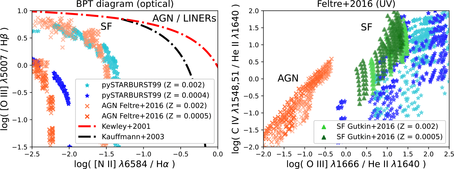
In the left panel of Figure 2, we plot our $Z=0.0004$ and 0.002 models with the corresponding AGN models of Feltre et al. (Reference Feltre, Charlot and Gutkin2016). It is clear that not only are the AGN models located in the traditional SF-dominated region of the BPT diagram, but they are also overlapping the distribution of SF models. Feltre et al. (Reference Feltre, Charlot and Gutkin2016) found that optical diagnostics are not useful in the low metallicity regime ( $Z\leq 0.008$ ). As alternatives, they proposed diagrams that use UV emission lines instead. In the right panel of Figure 2, the same models are shown in the C iv $\lambda\lambda$ 1548,51/He ii $\lambda$ 1640 versus O iii] $\lambda$ 1666/He ii $\lambda$ 1640 diagram. There are no diagnostic lines for this diagram, thus we also plot the corresponding SF models of Gutkin et al. (Reference Gutkin, Charlot and Bruzual2016). The models in this UV diagram are separated in well-defined areas dominated by SF and AGN.

Figure 2.

Left: BPT diagram showing our $Z=0.0004$ and $Z=0.002$ models of star-forming regions (SF) and AGN models from Feltre et al. (Reference Feltre, Charlot and Gutkin2016). Right: UV diagnostic diagram proposed by Feltre et al. (Reference Feltre, Charlot and Gutkin2016). SF models of Gutkin et al. (Reference Gutkin, Charlot and Bruzual2016) are also displayed.

4. WM-Basic, Fastwind and the He ii recombination lines

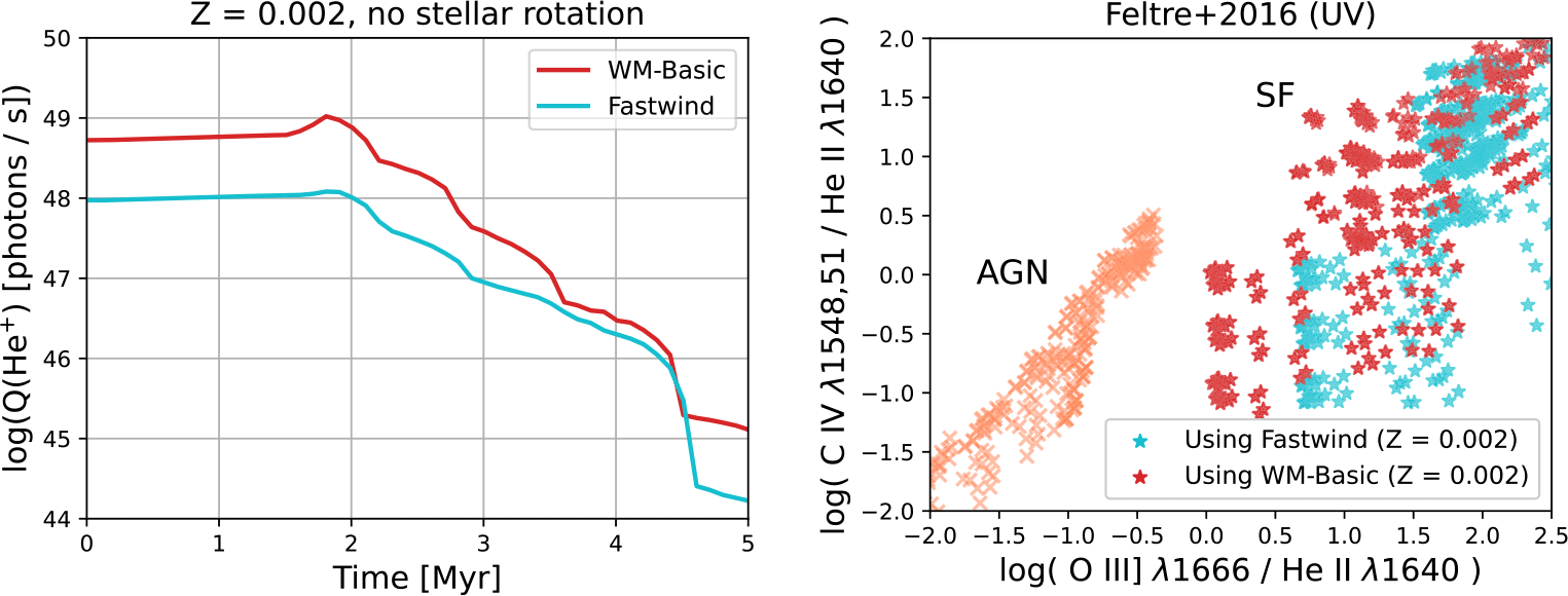
The 2014 release of Starburst99 uses WM-Basic (Pauldrach et al. Reference Pauldrach, Hoffmann and Lennon2001) stellar atmosphere models for main-sequence O-stars. Unfortunately, the closed-source code WM-Basic can not be modified in order to calculate spectra of VMS, nor population III stars. Instead, pyStarburst99 includes a completely new set of atmosphere models created using Fastwind (Puls et al. Reference Puls, Urbaneja, Venero, Repolust, Springmann, Jokuthy and Mokiem2005). In general, the emission line ratios predicted by using the Fastwind library are similar to those of WM-Basic for low and intermediate ionization ions. In the left panel of Figure 3 we compare the evolution of the predicted He ii ionizing flux of $Z=0.002$ models using Fastwind (red) and WM-Basic (blue). The WM-Basic models present a $\sim0.75$ dex higher flux than the Fastwind models. On the other hand, we do not notice as large a difference in the total H i ionizing flux between both sets of models (not shown here).

Figure 3.

Left: Evolution of He ii ionizing flux. Right: Comparison of $Z=0.002$ models using Fastwind (cyan) and WM-Basic (red) in the UV diagnostic diagram. Orange crosses same as in Figure 2.

The harder ionizing spectrum of WM-Basic models translates to a larger flux for highly ionized species (e.g., O iii, C iv, He ii). This is observed on the right panel of Figure 3. The models using WM-Basic show a shift to the left with respect of the Fastwind models as the He ii $\lambda 1640$ flux increases more relative to that of O iii] $\lambda 1666$ . The displacement in the ordinate is smaller as the ionization potential to produce He ii (54 eV) is closer to that of C iv (48 eV) than the one for O iii (35 eV).

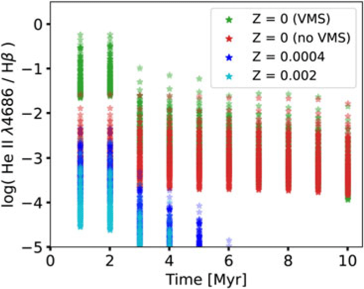
It is necessary to keep these changes in mind when He ii recombination lines are considered. This becomes relevant in the case of future studies of high-z galaxies potentially ionized by population III stars. In these environments, we expect to observe spectra dominated by H and He recombination lines. In Figure 4, the evolution of the He ii $\lambda$ 4686/H $\beta$ ratio is shown for low metallicity ( $Z\leq 0.002$ ) models without VMS. The ratio in models with population III stars remains high compared to the other metallicities. These stars remain in the main sequence longer than others as their only mass-loss mechanism is via critical rotation. For $Z=0$ , the presence of VMS in the first 3 Myr is noticeable with an increase of up to $\sim1$ dex in this ratio due to their harder ionizing spectrum.

Figure 4.

Evolution of the He ii $\lambda 4686$ / H $\beta$ ratio of models with $Z\leq 0.002$ .

5. Future work and access to the models

Version C25.00 of Cloudy was released recently (Gunasekera et al. Reference Gunasekera2025). Although further tests are required to completely assess the changes of this code for our purposes, the final grid will be calculated using this new version. Also, as previously stated, models with $Z=10^{-5}$ and 0.020 will be available for the full release of our grid.

Important outputs of the models will be available through the Mexican Million Models Database, 3MdB (Morisset et al. Reference Morisset, Delgado-Inglada and Flores-Fajardo2015). These include fluxes of over 300 nebular emission lines; ionic fractions and temperatures of all elements up to Zn; and physical characteristics of every model in our grid. The full potential of these photoionization models can only be exploited at its fullest with the help of the astronomical community.