INTRODUCTION
Monitoring trends in species abundance is an important part of conservation and management (Gray & Bewers, Reference Gray and Bewers1996); it attempts to identify and prevent undesirable outcomes of population management prior to their realization (Jennings et al., Reference Jennings, Kaiser and Reynolds2001). Monitoring is particularly important for populations of large mammals, where severe population crashes are relatively common (Young, Reference Young1994) and the causes not always known (e.g. Pitcher, Reference Pitcher1990; Thompson et al., Reference Thompson, Van Parijs and Kovacs2001; Gulland & Hall, Reference Gulland and Hall2007; Lonergan et al., Reference Lonergan, Duck, Thompson, Mackey, Cunningham and Boyd2007).
There has been considerable interest in the status of harbour seals (Phoca vitulina, Linnaeus 1758) in Europe due to fluctuations in population size. Historically, European harbour seal populations have been affected by hunting (Bonner et al., Reference Bonner, Vaughan and Johnston1973), pollution (Reijnders, Reference Reijnders1986) and disease (e.g. Dietz et al., Reference Dietz, Heide-Jørgensen and Härkönen1989; Härkönen & Heide-Jørgensen, Reference Härkönen and Heide-Jørgensen1990; Harwood & Grenfell, Reference Harwood and Grenfell1990; Heide-Jørgensen et al., Reference Heide-Jørgensen, Härkönen, Dietz and Thompson1992; Reijnders et al., Reference Reijnders, Ries, Tougaard, Nøgaard, Heidemann, Schwarz, Vareschi and Traut1997; Harding et al., Reference Harding, Härkönen and Caswell2002; Jensen et al., Reference Jensen, van de Bildt, Dietz, Andersen, Hammer, Kuiken and Osterhaus2002; Thompson et al., Reference Thompson, Lonergan and Duck2005). Elsewhere substantial declines in the number of harbour seals have been attributed to predation by sharks (Lucas & Stobo, Reference Lucas and Stobo2000), disturbance effects and competition with grey seals (Bowen et al., Reference Bowen, Ellis, Iverson and Boness2003). A number of other factors also drive the dynamics of seal populations, including immigration and dispersal (Bowen et al., Reference Bowen, Ellis, Iverson and Boness2003) and environmental variability, which influences individual reproductive success and survival (e.g. Trillmich & Ono, Reference Trillmich and Ono1991; Lunn et al., Reference Lunn, Boyd and Croxall1994). The relative importance of these factors for population size is not always clear. Moreover, although detecting changes in populations is often a requirement of conservation legislation, it can present considerable challenges.
Harbour seals spend much of their lives at sea and so are easiest to count when hauled out ashore (Summers & Mountford, Reference Summers and Mountford1975; Jemison et al., Reference Jemison, Pendleton, Wilson and Small2006). Longer haul-outs occur during the harbour seal pupping and moulting seasons, the timing of which has been consistent in the UK since surveys began in the 1980s (pupping: late May to early July, moulting: late July to early September). However, at no point in the annual cycle are all the animals in a population hauled out. Thus monitoring surveys do not provide an absolute abundance estimate, as some animals will always be missed. Instead an index of abundance, the minimum population estimate, is determined from the number of seals observed on land. In order to detect trends in abundance it is essential that the mean number of seals counted provides a consistent index of the number of animals in the survey area (Thompson et al., Reference Thompson, Tollit, Wood, Corpe, Hammond and MacKay1997).
Aerial surveys are considered to provide repeatable, consistent and accurate counts of seals in a short period of time (Pitcher & McAllister, Reference Pitcher and McAllister1981; Stewart & Yochem, Reference Stewart and Yochem1983; Yochem et al., Reference Yochem, Stewart, DeLong and DeMaster1987; Cunningham, Reference Cunningham2007). In the UK (e.g. SCOS, 2008) surveys take place during a three-week survey window (31 July to 23 August) within the annual moult when, in most areas, the greatest numbers of seals are hauled ashore (Thompson & Harwood, Reference Thompson and Harwood1990; Boveng et al., Reference Boveng, Bengtson, Withrow, Cesarone, Simpkins, Frost and Burns2003; Harris et al., Reference Harris, Lelli and Gupta2003). The survey window is further restricted to within two hours of low tide when the greatest numbers of harbour seals are thought to be ashore (Allen et al., Reference Allen, Ainley, Page and Ribic1984; Yochem et al., Reference Yochem, Stewart, DeLong and DeMaster1987; Thompson et al., Reference Thompson, Fedak, McConnell and Nicholas1989; Watts, Reference Watts1996; Simpkins et al., Reference Simpkins, Withrow, Cesarone and Boveng2003). Poor weather can reduce the number of seals hauled out on a given day (e.g. Godsell, Reference Godsell1988; Kovacs et al., Reference Kovacs, Jonas and Welke1990; Grellier et al., Reference Grellier, Thompson and Corpe1996), especially during the moult when animals probably haul out to increase their skin temperature (Boily, Reference Boily1995). Therefore in the UK aerial surveys only take place in dry weather.
It is assumed that, by carefully selecting the environmental condition and the timing of aerial surveys, many of the factors that could cause variation in counts will be eliminated. However, different demographic components of the population differ in the timing of the moult and it is likely that the timing and duration of the moult plateau will alter if there are changes in the demographic structure of a population (Härkönen et al., Reference Härkönen, Harding and Lunneryd1999; Daniel et al., Reference Daniel, Jemison, Pendleton and Crowley2003). It is therefore important to include an estimation of the variance in the number of seals hauled out during the survey period.
This study modelled land-based counts from a single haul-out site on the Isle of Skye, north-west Scotland, obtained between May and September 2004 and 2005, in order to: (i) gain a better understanding of how temporal, tidal and environmental covariates affect the numbers of seals hauled out in Scotland; (ii) determine whether numbers of animals remain stable during the moult; and (iii) assess whether this period coincides with the aerial survey window. In addition, five repeat aerial surveys of haul-out sites around the Isle of Skye, were conducted in August 2004 and these were used to calculate a coefficient of variation (CV) and determine a minimum abundance estimate (i.e. seals counted at haul-out sites) that could be used as a baseline in the management of this harbour seal population.
MATERIALS AND METHODS
Land-based counts
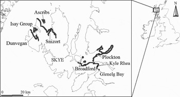
Land-based counts were carried out at Kyle Rhea, which is a seawater channel located between the Isle of Skye and the north-west coast of mainland Scotland (57°14′N 5°39′W; Figure 1). The number of harbour seals hauled out was observed between May and September in 2004 and 2005. All observations took place at distances no greater than 1 km from the seals and were made using 7 × 50 binoculars. Environmental variables (wind strength and direction, cloud cover (%), precipitation, water flow direction and speed), chosen for their potential influence on seal numbers and their measurability, were approximated by sight as detailed below. Data on the predicted time and height of the tides were taken from POLTIPS using Glenelg Bay as the reference port.
Location map of the tidal port, Glenelg Bay, and the Kyle Rhea haul-out site on the Isle of Skye, north-west Scotland. The seals hauled out were counted from both sides of the channel. Repeat aerial survey tracks around the Isle of Skye are shown. Northern sub-areas: Dunvegan, Isay Group, Ascribs and Snizort; southern: Plockton and Broadford.

To investigate the effects of temporal, tidal and environmental covariates on harbour seal behaviour it was assumed (based on personal observation around the Isle of Skye) that the haul-out patterns shown in Kyle Rhea were representative of the broader region included in the aerial surveys. The data collected during 2004 were used to fit the model (calibration data set), and data collected in 2005 constituted an independent validation data set. Environmental variables were compared between the model fitting and validation data sets using Mann–Whitney tests to ensure that general environmental conditions were comparable between years. All variables were also examined for co-linearity using Pearson product–moment correlation tests.
Generalized additive model
To account for any over-dispersion resulting from count data, a quasi-Poisson distribution was used with a generalized additive model (GAM) to attempt to describe the factors that may affect the number of seals hauled out, and thus available to be counted, during aerial surveys. The following explanatory variables, and their interactions, defined the upper limit of the multivariate regression model: time of day, time since low tide, time of nearest low tide (all in decimal hours), tide height, height of nearest low tide (in metres) and Julian date were modelled as smooth non-metric functions; tide state (high, ebbing, low, flooding or slack), precipitation (absent, mist, drizzle, light rain, heavy rain, hail, sleet or snow), cloud cover (to nearest 25%), wind strength (calm, gentle breeze, light wind, strong wind and gale force winds), wind direction and water flow speed (slow, medium or fast) were modelled as categorical factors. The direction of water flow was highly correlated with the state of the tide (Pearson's product r = –0.781, P < 0.001) and so was not included in the full model. A circular smooth was used to account for the circularity of the tidal state, but was not needed for ‘time of day’ as no counting took place at night. Because individual seals could have been hauled out during consecutive counts (Cunningham et al., Reference Cunningham, Baxter, Boyd, Duck, Lonergan, Moss and McConnell2009) the residuals were checked visually for non-randomness in the data. Some positive correlation with the previous count, rather than the mean number of seals hauled-out, was apparent. Consequently, to eliminate the complications associated with serial correlation in the data and so that each count could be considered independently, only alternate records were used for the model.
A combination of backward and forward stepwise selection was used to determine the best-fitting model. Starting with a model containing all the covariates, the effect of deleting variables was evaluated at each step, with those variables not contributing significantly to the fit of the model being placed into a pool of candidate variables from where they could be reselected. Candidate models were specified in R using function gam(mgcv) (Wood, Reference Wood2001). The predicted number of harbour seals hauled out was obtained using the best-fitting model and function predict.gam(mgcv) in R. The daily mean number of harbour seals predicted to be hauled-out was calculated at five-minute intervals within a four-hour tidal window because the probability of surveying was considered to be equal within this four-hour period.
Cross-validation between calibration and validation data sets (Burnham & Anderson, Reference Burnham and Anderson2002; Olden et al., Reference Olden, Jackson and Peres-Neto2002) was used to assess whether the best-fitting model captured a persisting biological relationship between temporal, tidal and environmental variables and the observed numbers of harbour seals hauled-out. The effect of increasing the number of knots from three to seven was observed to ensure that the best-fitting GAM was robust.
Aerial surveys
Harbour seals on the south-east and north-west coasts of the Isle of Skye (Figure 1) were counted on five consecutive days during the annual moult (2–6 August 2004) using a thermal imaging camera mounted in a helicopter. Aerial counts were only carried out during the early afternoon, within two hours of low tide and only in dry weather in order to reduce the potential effects that date, time of day, tide and weather might have on the counts. One survey (3 August) was conducted in light to moderate drizzle when aerial counts would not usually have taken place.
The camera had a dual telescope with ×2.5 and ×9 magnifications and was mounted alongside a Hi8 camcorder, recording onto VHS and Hi8 tapes respectively. Flying at around 180 m height, the coast was scanned at low magnification; groups of seals were counted in real time using high magnification when they were detected. Species identity was determined using the thermal profile of the seals, the real image from the camcorder, or using binoculars. The size and location of each group were recorded onto 1:50,000 Ordnance Survey maps and later transcribed into a database.
The aerial survey route was divided into sub-areas (Dunvegan, Isay Group, Ascribs and Snizort in the north, Plockton and Broadford in the south; Figure 1) to allow trends in abundance of similarly sized groups of harbour seals to be compared. Although care was taken to divide the overall survey area in places where few seals were found, the sub-areas do not represent distinct populations. The mean abundance estimate for each sub-area was calculated from the replicate counts and a CV was determined for each sub-area and for the survey area as a whole. A Wilcoxon signed-ranks test was used to determine which days showed significant change in abundance. All analyses were compared between ‘all surveys’ (which included the wet-weather count when counts would not usually occur) and ‘dry surveys’ (which discounted data from 3 August).
RESULTS
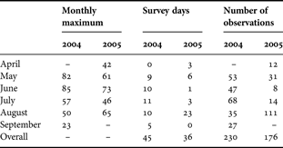
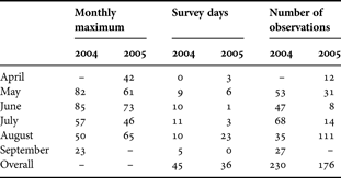
Data for harbour seals hauled out in Kyle Rhea were collected over 45 days in 2004 and 36 days in 2005, producing a total of 406 observations. The maximum number of seals, excluding pups, observed each month varied from 23 in September (9) to 85 in June (11) (Table 1).
Data collected from land-based counts of harbour seals hauled out in Kyle Rhea, north-west Scotland. Hourly observations were conducted to capture tidal, temporal and environmental variation in the number of harbour seals counted on each survey day.
Environmental variables were compared between the model calibration and validation data sets to ensure that general environmental conditions were comparable between years. Only wind strength had a slightly higher median value in 2005 compared to 2004 (Mann–Whitney U: z = −3.334, P = 0.001). A number of variables were significantly correlated but these correlations were weak (all r < 0.3, except precipitation and cloud cover where r = 0.42) and were probably a result of the categorization of the variables.
With a log link function and a quasi-Poisson distribution the final GAM took the form:

where log(E(PV)) is the log link function of the independent response variable (numbers of harbour seals hauled out), β 0 is the intercept and β 1 and β 2 are the estimated coefficients of the respective variables (jdate = Julian date; time_since = time since low tide) and s is a circular smooth function of covariates β 1 and β 2. No interactions improved the model fit. Visual inspection of the deviance residuals gave no reason to suspect non-randomness in the data for either the calibration or the validation data. The fit of the model using the calibration data set (collected in 2004, N = 115) explained 62.5% of the variance (R-squared = 0.56), compared with 38% of the variance (R-squared = 0.31) for the validation data set (collected in 2005, N = 88). The variances of errors in the prediction models were 8.27 for the calibration data set and 7.52 for the validation data set.
The prediction model, determined as the best-fitting model from the calibration data set, was not the best-fitting model for the validation data set when using the same model selection procedure. However, the ΔGCV between the best-fitting model for the validation data and the prediction model was small (−1.410). Thus the difference between the candidate model proposed by the validation data set and the prediction was deemed sufficiently small (Brown & Mate, Reference Brown and Mate1983), and the more parsimonious prediction model (above) was selected. Increasing the number of knots had little effect on the predicted relationship between numbers hauled out and time of year and time since low tide. Using more knots in the model resulted in a prediction of a slightly higher count of harbour seals during the pupping season (July, though this was still lower than May/June and August peaks), and a more sudden increase in harbour seals during the ebbing tide.
Temporal and tidal variation
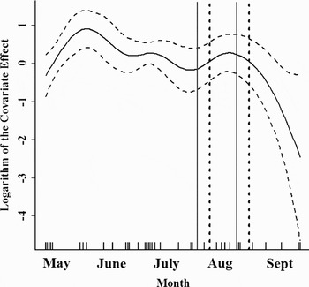
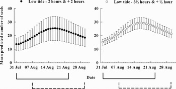
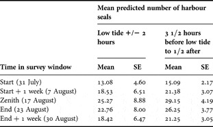
Between May and September highest counts of seals were predicted during the pupping season (86 seals on 27 May, compared to a maximum of 85 observed on 11 June). The longest period of high seal counts occurred during the moult and coincided with the aerial survey window (Figure 2). However, predicted numbers of seals (from two hours before until two hours after low tide) were lower at the peak's zenith on 17 August than at either the start or end of the normal window (Table 2); due to the nature of a GAM, and a relatively small land-based count data set, seal numbers appeared to peak rather than plateau within the survey window (Figure 3).
The effect of date, a smooth term component of the generalized additive model, for land-based counts of harbour seals in south-east Skye. Upper and lower curves represent two standard errors above and below the estimate (approximate 95% confidence intervals). Vertical solid lines represent the start and finish of the normal survey window and horizontal dashed lines show the start and finish of a survey window delayed by one week. The y-axis is the logarithm of the covariate effect. The rug plots at the foot of the graphs show when counts were actually made.

Daily mean number of harbour seals (with standard error) predicted to be hauled out in Kyle Rhea, north-west Scotland, from two hours before until two hours after low tide (•) and from 3 1/2 hours before until half and hour after low tide (○). Solid lines represent the start and finish of the normal survey window, from 31 July until 23 August, and dashed lines show a three-week survey period starting one week later (7–30 August).

Mean predicted number of harbour seals hauled ashore calculated from five-minute intervals during two four-hour tidal periods. The predicted number of seals is shown for the start, zenith, end and end + 1 week of the normal three-week aerial survey window in dry weather.

Only a few counts were carried out in early May and in September, and so the predicted effect of early and late season on seal counts is imprecise. Nevertheless, although the aerial survey window coincided with the predicted peak in numbers of harbour seals during the moult, delaying surveys by a period of one week would reduce the variability between counts of seals hauled out in Kyle Rhea during the survey window (Table 2; Figure 3).
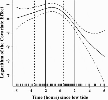
Seal numbers increased during the ebbing tide, with highest numbers observed from about 3 1/2 hours before low tide until half an hour after (Figure 4). Numbers of harbour seals ashore decreased rapidly during the flooding tide, with approximately six times fewer animals hauled out two hours after low tide, compared with the peak at around one hour before low tide.
The effect of time since low tide, on numbers of seals hauled out. A peak in numbers of harbour seals was predicted at one hour before low tide (mean predicted number of seals = 29.58, SE = 6.02). Vertical solid lines represent the start and finish of the normal survey window, from two hours before until two hours after low tide, and horizontal dashed lines show 3 1/2 hours before to 1/2 hour after low tide (21.4 seals, SE = 6.02; 18.88 seals, SE = 3.84 predicted respectively).

Surveying harbour seals 1 1/2 hours earlier in the tide, from 3 1/2 hours before to 1/2 hour after low tide, increased the mean daily predicted number of seals and reduced the variance by about half (Table 2; Figure 3).
Repeat aerial surveys
As predicted by the GAM, seal counts did not remain constant during the repeat aerial surveys conducted over five consecutive days at the beginning of the survey window, but increased between the start and finish of the study period (2 to 6 August, Wilcoxon signed-ranks: Z = –1.99, P = 0.046; the increase between 3–4 and 4–5 August was significant at the 0.05 level: Z = –1.99, P = 0.046 and Z = –2.20, P = 0.028 respectively).
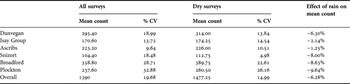
In most cases the CV (defined as the standard error of the mean expressed as a proportion of the mean) around the mean of the counts, obtained using a thermal imager from a helicopter was reduced when calculated without the wet survey. The mean of the individual CVs, and the CV of the total counts was 15% (Table 3). Counts of harbour seals were lower on the wet day (3 August) than the dry days; the effect varied considerably from a 1.3% decline in the Ascribs, to an over 9.5% decline in the Plockton area (Table 3). The overall mean harbour seal count decreased by 6.3% when the count obtained during the wet weather survey was included.
Mean counts and coefficient of variations (CV) of harbour seals in different sub-areas around the Isle of Skye calculated from repeat dry-weather aerial surveys (‘dry surveys’) and from all aerial surveys including one wet-weather count (‘all surveys’). The effect of including data from wet-weather surveys is determined by the percentage change in the mean count from ‘dry surveys’ to ‘all surveys’.

DISCUSSION
Harbour seal abundance surveys are designed to reduce the effect of variation in the numbers of seals hauled out by reducing the number of environmental variables that are likely to affect the counts and by attempting to carry out surveys at the same time within the tidal and life-cycle. However some factors, such as prey availability, habitat type and disturbance (e.g. Brown & Mate, Reference Brown and Mate1983; Allen et al., Reference Allen, Ainley, Page and Ribic1984; Thompson et al., Reference Thompson, Tollit, Wood, Corpe, Hammond and MacKay1997) that may affect haul-out behaviour cannot be controlled for and even control of some of the focal environmental variables can be imperfect. Some studies have also shown that there are site-specific variations in harbour seal behaviour patterns depending on factors such as habitat type (Thompson et al., Reference Thompson, Tollit, Wood, Corpe, Hammond and MacKay1997). In this study, on rocky habitat in north-west Scotland, two covariates, ‘time since low tide’ and ‘date of survey’, comprised the best-fitting GAM, the predictions of which were robust to changing the number of knots in the model. Interestingly, ‘time of day’ was not important in the final model, thus the current practice of restricting surveys to the afternoon does not appear to be important in this region.
There has been some debate over the effect of precipitation on the number of harbour seals seen hauled out. Godsell (Reference Godsell1988) found a significant correlation, Grellier et al. (Reference Grellier, Thompson and Corpe1996) a weak correlation, and Kovacs et al. (Reference Kovacs, Jonas and Welke1990) no relationship at all. However, rain probably decreases the ability to detect seals with the thermal imager so that including data from the wet day decreased the mean harbour seal aerial count in this study by 6.3%. However, there was considerable spatial variation in the observed effect of precipitation on numbers of seals, which could be due to differences in the strength, duration and direction of inclement weather as well as the availability of alternative, more sheltered, haul-out sites. The covariate precipitation was not deemed sufficiently important to remain in the predictive model, probably as a result of spatial variation in effect. Due to these observed spatial differences it is not advisable to use a correction factor to adjust wet-weather aerial surveys to estimate the number of animals hauled out under ‘ideal conditions’ (e.g. Boveng et al., Reference Boveng, Bengtson, Withrow, Cesarone, Simpkins, Frost and Burns2003; Simpkins et al., Reference Simpkins, Withrow, Cesarone and Boveng2003) for such a large survey area.
Peaks in numbers of harbour seals hauled out around low tide have been observed both in areas where haul-out sites are only available at low tide (e.g. Thompson et al., Reference Thompson, Lonergan and Duck2005), and elsewhere (e.g. Schneider & Payne, Reference Schneider and Payne1983; Allen et al., Reference Allen, Ainley, Page and Ribic1984; Frost et al., Reference Frost, Lowry and Ver Hoef1999; Boveng et al., Reference Boveng, Bengtson, Withrow, Cesarone, Simpkins, Frost and Burns2003). The GAM in this study predicted highest numbers of harbour seals hauled out one hour before low tide, with a gradual build up in seal numbers during the ebbing tide and a more rapid decline during the flooding tide. The narrow channel at Kyle Rhea causes rapid tidal flooding, and this may have had some effect on the time when the maximum number of harbour seals was ashore. Thus the results of this study are not necessarily valid at all other harbour seal haul-out sites in the UK. Nevertheless, this study indicates that surveys of seals hauled out in Kyle Rhea conducted 1 1/2 hours earlier than the normal survey time will result in higher and less variable counts. It is likely that survey windows may therefore be site-or region-specific.
In the past the approach adopted for surveying harbour seals was to survey when numbers were highest and most consistent. This can occur either during the pupping (e.g. Brown & Mate, Reference Brown and Mate1983; Thompson et al., Reference Thompson, Tollit, Wood, Corpe, Hammond and MacKay1997; Huber et al., Reference Huber, Jeffries, Brown, DeLong and Van Blaricom2001) or moulting (e.g. Thompson et al., Reference Thompson, Fedak, McConnell and Nicholas1989; Boveng et al., Reference Boveng, Bengtson, Withrow, Cesarone, Simpkins, Frost and Burns2003; Harris et al., Reference Harris, Lelli and Gupta2003) period. The highest number of adult harbour seals observed hauled out in this study occurred during the pupping season (late May to early July) although numbers of seals declined rapidly after this peak. In contrast, although fewer animals were counted during the moult period (August), the numbers were less variable. Numbers of harbour seals in this study were therefore highest during the pupping season but most consistent during the moult, possibly reflecting the age and sex composition of the haul-out site.
The raised temperature of moulting seals increases their visibility, and therefore detectability, on the thermal imager (Sharples, Reference Sharples2005), which is currently the favoured device for counting seals on rocky shores in Scotland. Not only are counts made during the moulting period more consistent than those made during the pupping season, but the error associated with these moult counts may also be less than during the pupping season. Furthermore, during the pupping season a higher proportion of breeding seals may be ashore compared to non-breeders and consequently haul-out behaviour would not be recorded from a random sample of seals as it should (Southwell, Reference Southwell2005). This could affect population estimates unless correction factors, used to convert counts into population estimates, were equally biased. However, counts during the pupping season are more sensitive to short-term changes in reproductive success than those obtained during the moult. Surveys conducted during the pupping season, rather than during the moult, may therefore be more appropriate for assessing the conservation status of harbour seals and initiating timely response to any changes in population size.
Counting harbour seals to provide an estimate of minimum population size assumes that the survey window covers a period when there is no significant trend in numbers hauled out. However, the predicted number of harbour seals in this study did not plateau during the survey window; instead a peak was observed with the zenith of the predicted number of harbour seals hauled out occurring during the final quarter of the normal survey window. Harbour seals moult at different times according to their location, sex- and age-class (e.g. Thompson & Rothery, Reference Thompson and Rothery1987; Härkönen et al., Reference Härkönen, Harding and Lunneryd1999; Daniel et al., Reference Daniel, Jemison, Pendleton and Crowley2003). Animals are therefore likely to moult in pulses, with males spending more time ashore at the end of the moult period (Thompson et al., Reference Thompson, Fedak, McConnell and Nicholas1989) and yearlings being the first to moult (Thompson & Rothery, Reference Thompson and Rothery1987). This may explain why a plateau in seal numbers was not observed, although it could also have been influenced by the nature of the GAM. Alternatively a plateau may have occurred subsequent to the repeat surveys in this study, perhaps delayed as a result of a shift in the timing of pupping and the moult as observed in harbour seals elsewhere (e.g. Jemison & Kelly, Reference Jemison and Kelly2001; Daniel et al., Reference Daniel, Jemison, Pendleton and Crowley2003).
Coefficient of variation
Although the average variation among sub-areas may have provided a lower CV than for the mean CV for the combined aerial survey counts (i.e. 15%, c.f. Lonergan et al., Reference Lonergan, Duck, Thompson, Mackey, Cunningham and Boyd2007), it assumes independence between sub-areas, i.e. no movement of animals between the sub-areas, which is known not to be the case in at least part of the study area between September and July (Cunningham et al., Reference Cunningham, Baxter, Boyd, Duck, Lonergan, Moss and McConnell2009). The spatial variation in the CV may have been due to local environmental influences affecting haul-out behaviour on a relatively small spatial scale. However, the timing and height of the tide at the time of the repeat aerial surveys were similar in each area, and there were no notable weather differences during the four-hour survey periods. Consequently, at present this is the most appropriate CV for aerial surveys of harbour seals in Scotland.
Repeat counts at haul-out sites provide a measure of uncertainty that is associated with a single count; information that is essential to determine the statistical significance of any observed changes in the number of seals using that site. However, the high levels of variation observed in this study mean that only large changes in seal counts can be detected using aerial surveys. Some of this variability, which is the result of variations in haul-out behaviour among individuals (e.g. Brown & Mate, Reference Brown and Mate1983; Thompson et al., Reference Thompson, Fedak, McConnell and Nicholas1989; Cunningham et al., Reference Cunningham, Baxter, Boyd, Duck, Lonergan, Moss and McConnell2009) and among age- and sex-classes (Härkönen et al., Reference Härkönen, Harding and Lunneryd1999), cannot be reduced by improvements in survey design. However, variability in haul-out behaviour that is the result of responses to different environmental conditions can be addressed if a statistically significant relationship between haul-out behaviour and these covariates can be established. Understanding the uncertainty surrounding counts is therefore fundamental to determining the status of the population, which is a requisite for the effective management and conservation of marine mammals (Small et al., Reference Small, Pendleton and Pitcher2003). For harbour seals in the European Union, reporting on the conservation status of harbour seals is also a legal requirement under the EC Habitats Directive. To comply with this requirement, changes in seal counts at haul-out sites need to be detected so that timely management decisions can be made. Further work is needed to determine the temporal and spatial variation in optimal aerial survey windows for harbour seals across the remainder of the UK harbour seal population. The present study has demonstrated several sources of variance in methods used to count numbers of seals hauled out, which is used as an index of harbour seal abundance, and shown the type of variation that might be expected elsewhere. Incorporating these, and defining covariates such as the timing of the moult, within estimation methods will improve the estimation of population size from periodic counts and it will also increase our ability to detect trends in abundance.
ACKNOWLEDGEMENTS
Thanks to Dave Clem and Callan Duck for their help with the aerial surveys, and to Beryl Bannister, Gemma Danks, Colin MacDonald and Murray Morrison for their help counting seals amidst midges. Thanks also to Peter Cunningham for his dedication to the project and to Beth Mackey for her comments on previous versions of the manuscript. This work was funded by Scottish Natural Heritage, with contributions from the Sea Mammal Research Unit and Highland and Islands Enterprise.