1. INTRODUCTION
The vehicle routing problem (VRP) is a generic name referring to a class of combinatorial optimization problems in which customers are to be served by a number of vehicles. The vehicles leave the depot, serve customers in the network, and on completion of their routes return to the depot. In other words, VRP involves designing of a set of routes for a fleet of vehicles, starting and ending at a depot and serving a number of customers with known demands. Each customer must be visited by one of these routes, and the objective is to minimize the global cost of the set of routes.
Theoretical research and practical applications in the field of vehicle routing started in 1959 with the truck dispatching problem posed by Dantzig and Ramser (Reference Dantzig and Ramser1959). Using a method based on a linear programming formulation, their hand calculations produced a near-optimal solution with four routes to a problem with 12 service stations. The authors proclaimed: “No practical applications of the method have been made as yet.”
In the nearly five decades since Dantzig and Ramser's (Reference Dantzig and Ramser1959) paper appeared, more specific work in the field has exploded dramatically. The VRP has extensive variants, including periodic VRP (PVRP, in which the customers are served in a period of time rather than 1 day), VRP with pickup and delivery (VRPPD, in which the customers may both receive and send products), VRP with time windows (VRPTW, in which the vehicles must arrive at the customers before the latest arrival time, while arriving before the earliest arrival time results in waiting), multidepot VRP (MDVRP, in which more than one depot is considered), multidepot PVRP (MDPVRP), and so on (Dantzig & Ramser, Reference Dantzig and Ramser1959). In the case of MDVRP, the decision makers also have to determine which customers are served by which depots, that is, the grouping problem prior to the routing and scheduling problems. The MDPVRP reduces to a PVRP when there is one depot and to a MDVRP when there is no periodic service.
Over the last 50 years or so, the classical VRP has been strongly attended in the literature compared to the fewer research projects on the PVRP, MDVRP, and MDPVRP.
Drummond et al. (Reference Drummond, Ochi and Vianna2001) proposed an island-based parallel evolutionary method for the PVRP, which evolves individuals representing schedules (patterns), the fitness of each individual being obtained by constructing routes for each period with a saving heuristic. In 2007, scatter search procedure was especially developed just for solving PVRP when the number of periods is large (Alegre et al., Reference Alegre, Laguna and Pacheco2007). In this research like what happened in Drummond et al., schedule improvement and route design were considered as two key focuses to solve the problem respectively. In contrast to these researches, Matos and Oliveira (Reference Matos and Oliveira2004) focused on routes optimization at first and then scheduling phase. They developed an effective ant colony optimization for PVRP.
Local optimum is one challenging point in PVRPs. To escape this situation, Chao et al. (Reference Chao, Golden and Wasil2007) used a local search approach and showed that it works effectively when vehicle capacity constraint is relaxed. Tabu search was another heuristic that was used by Cordeau et al. (Reference Cordeau, Gendreau and Laporte1997, Reference Cordeao, Laporte and Mercier2001) in basic and unified format. This approach is considered as the state of the art solution approach for a number of VRP variants, especially for the PVRP and the MDVRP, for a long period of time. They also formulated PVRP. Hemmelmayr et al. (Reference Hemmelmayr, Doerner and Hartl2009) outperformed previous approaches by the variable neighborhood search that was built upon various well-known VRP neighborhoods. Finally, multilevel refinement strategy of this kind of neighborhood search was developed by Pirkwieser and Raidl (Reference Pirkwieser, Raidl, Cowling and Merz2010).
For the MDVRP, a few researchers have taken advantage of geometric aspects within the problem. Thangiah and Salhi (Reference Thangiah and Salhi2001) introduced a mutation operator that targets the depot assignment to “borderline” customers, which are close to several depots. In this regard, some approaches are considered more effective, for example, methods based on neighborhood search like the Tabu search algorithms (Renaud et al., Reference Renaud, Laporte and Boctor1996; Cordeau et al., Reference Cordeau, Gendreau and Laporte1997) and simulated annealing (Lim & Zhu, Reference Lim and Zhu2006). Pisinger and Ropke (Reference Pisinger and Ropke2007) have attacked the MDVRP by an adaptive large neighborhood search method, which implements the ruin and recreate paradigm with adaptive selection operators. Ho et al. (Reference Ho, Ho, Ji and Lau2008) developed two hybrid genetic algorithms (HGAs) for MDVRP. The major difference between the HGAs was the initial solutions. Giosa et al. (Reference Giosa, Tansini and Viera2002) presented new assignment algorithms for the MDVRP, and Crevier et al. (Reference Crevier, Cordeau and Laporte2007) addressed an extension of the MDVRP in which vehicles may be replenished at intermediate depots along their routes.
It was very hard for authors to find research on MDPVRP. In this respect, a Tabu search based method was considered by Parthanadee and Logendran (Reference Parthanadee and Logendran2006) for MDPVRP when backorder is allowable. In addition, Crainic et al. (Reference Crainic, Crisan, Gendreau, Lahrichi and Rei2009) developed the integrative cooperative search approach, by problem decomposition and adaptive search guidance mechanisms. Finally, Vidal et al. (Reference Vidal, Crainic, Gendreau, Lahrichi and Rei2012) proposed an algorithm framework addressing MDPVRP with capacitated vehicles and constrained route duration.
A number of exact methods have also been suggested for the problems addressed. The recent contributions of Baldacci and Mingozzi (Reference Baldacci and Mingozzi2009) and Baldacci et al. (Reference Baldacci, Bartolini and Mingozzi2011) addressing the MDVRP and the PVRP are noteworthy. Exact methods are limited in the size of instances they may handle, but these particular approaches have proven quite successful in optimizing several instances that are used as a test bed for the algorithm proposed.
This brief review reveals that the contributions to the MDPVRP literature are very scarce. By a general glance at the real-world problems, we can find that a large number of problems can exactly match the new classification of the MDPVRP concepts. For more explanations, consider the following problems encountered that are based on the author's experiences:
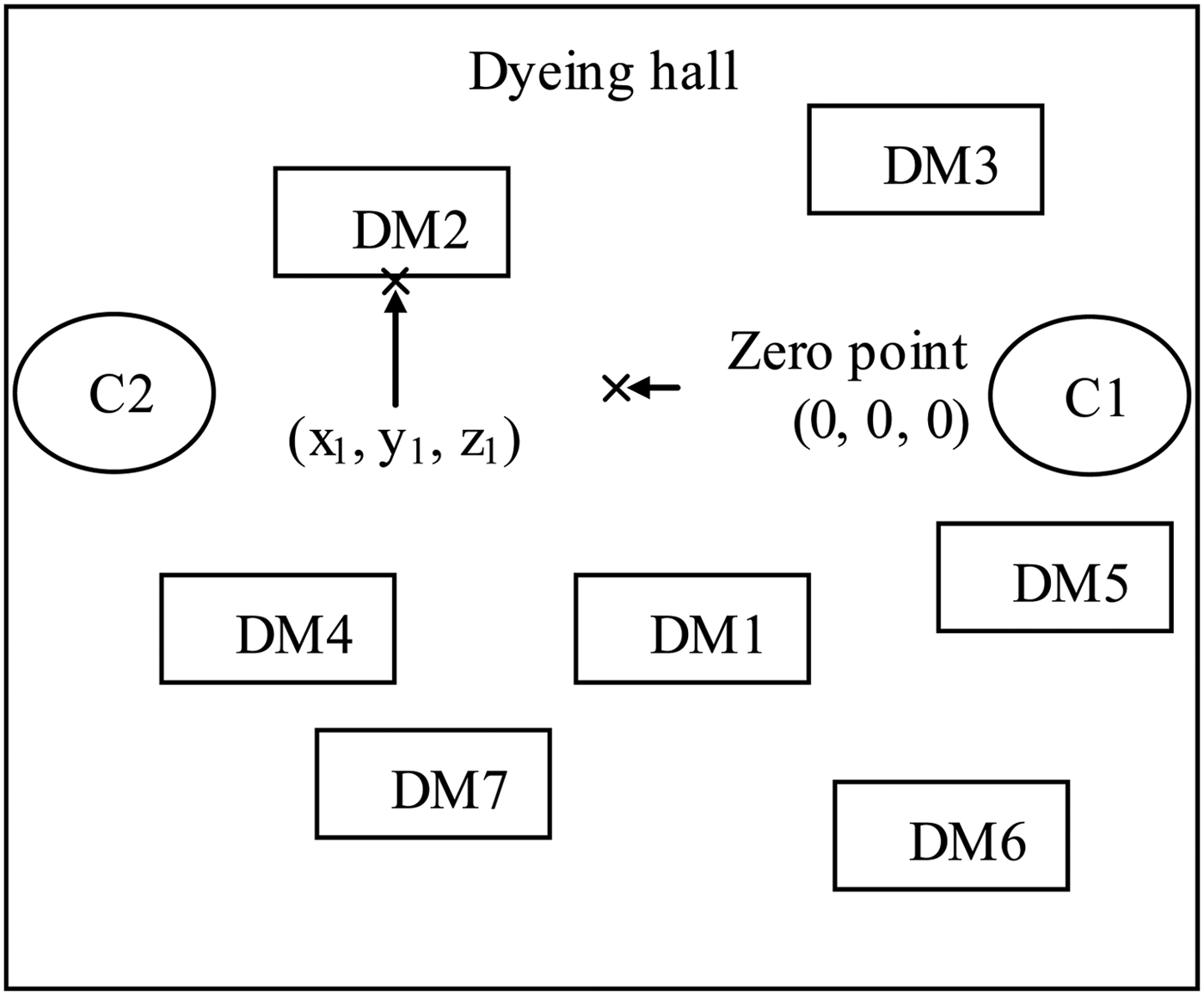
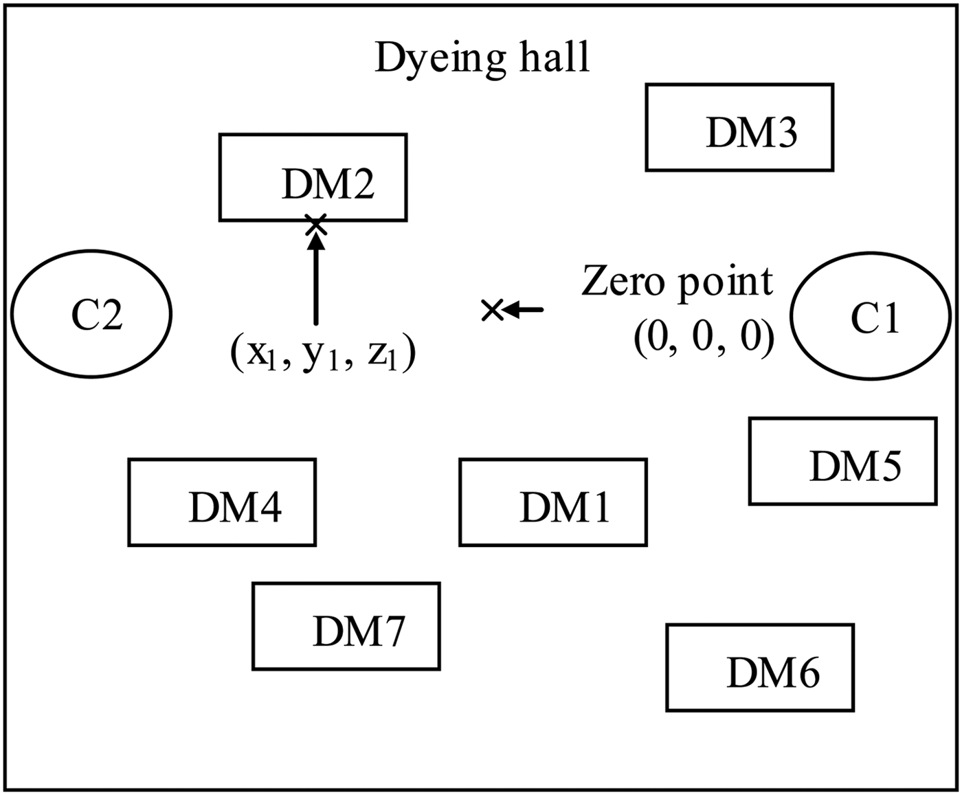
Textile industry: In the dyeing process of all kinds of fibers, there are several dyeing machines (customers), several cranes (vehicles), and one or more parking sites (depots). The cranes carry the basket filled with wet fiber toward the dyeing machines and put it into them. The route traveled by the crane is not the least distance and moves across the x, y, and z axes. When the dyeing process is finished, the machine needs the crane again to put another full basket into it. The crane does not come back to its depot until there is no machine needing it. Therefore, the vehicle starts its trip, serves some customers, and then comes back to its depot. Processing times are fixed, and each machine needs the crane during each constant time interval. In this kind of MDPVRP, when the vehicle starts its trip, it is scheduled to service some constant number of customers. However, during its trip, some dyeing machines (known as new customers) that may not have needed service at the starting time of the trip are added to its customers to take service after ending their dyeing process. Therefore, the first schedule may not be valid until the end of trip because some new customers can be added. Hence, it would be desirable to minimize not only the total traveled distance but also the total waiting time of all customers. A general overview of this problem is illustrated in Figure 1.
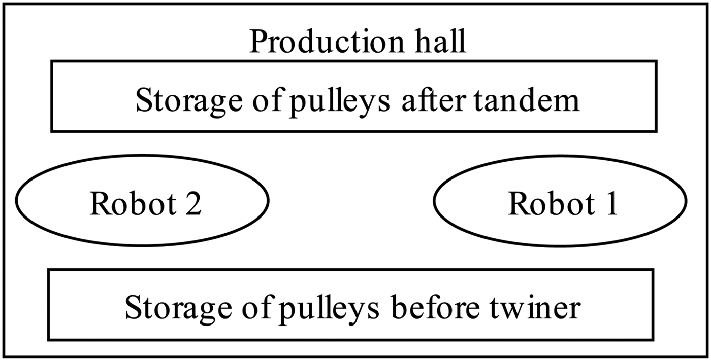
Cable industry: A similar condition can be witnessed in the cable industry. Three kinds of cable (air core, jelly, and aerial) are produced in three stages called tandem, twiner, and strander. One expert robot works between the tandem stage and twiner, and another between the twiner stage and strander. The robots are located and fixed at the corners. They move toward each spool (pulley) through three axes (X, Y, and Z), fixing some settings (like fixing the position of pulley, checking its thickness, its color). Then the pulley moves to the next stage, and it is replaced by a new pulley with the same demand. A robot does not return after starting its trip, unless no pulley needs setting. Delays in the setting process lead to reduction in the quantity of production, and the longer the trip takes, the more costly it is. Therefore, waiting time of the customer and the traveled distance of the vehicle are important factors to consider. Here also some new pulleys (customers) waiting service may be added, while the robots complete their trip. It should be noted that robots take a large space in three dimensions, and when more than one robot is needed, they must be located at two opposite sites (multidepot). Figure 2 provides a general view of a typical production hall in the cable industry.
Electronic industry: In the production process of electronic boards, robots move toward each board to fulfill some of their requirements. In this case, the robot has a deterministic position (depot). When some actions are needed to be done on one or more boards, the robot starts its trip toward them to perform the required actions. A robot is devised to move in least distance between depot and a board or between two boards. The boards must wait for service, in case their number is more than the number of vehicles. Here again, some new boards may be added as new customers waiting for service during robot traveling. Finally, by the time there are no more boards needing service, the robot can return to its depot.
Two cranes (C1 and C2) and seven dyeing machines (DM1 to DM7).
Two robots between tandem and twiner stages.

By observing all the above-mentioned cases and also many other similar cases observed in the industrial world, there would be an incentive to think of a new issue of MDPVRP. Such a new definition must be adaptable to all these various cases. Therefore, the main contribution of this research would be considering a new kind of MDPVRP in which customer sequencing in each route (for getting service) can be changed based on the number of new customers added to service line. Two criteria play the key role as our objective function: total traveled distance at each depot and total waiting time of all customers to take service. This research also attempts to develop an effective genetic algorithm (GA) approach to solve the problem. The developed GA in this study is augmented by some effective local searches, a modified approach to generate initial population, an improved heuristic to improve initial solutions, and also one heuristic mutation none of the previous researchers have mentioned.
The definition of the classical VRP includes determining a set of m vehicle routes with each rout starting and ending at the depot, minimizing total traveling cost of vehicles, and making sure each customer is visited exactly once by exactly one vehicle.
In the presented MDPVRP, there are n customers and m vehicles located in k depots. Each customer i works independently for a fix time (t i) and then will be stopped, needing a vehicle to take service. To solve this problem, we follow three stages called grouping, routing, and scheduling. After allocating each customer to a specific depot (grouping), each customer should be allocated to a specific vehicle located in the related depot (routing). When one or more customers are stopped, the allocated vehicle should leave its depot and start the trip. If just one customer needs service, there is no such problem as scheduling, but when there is more than one customer, the vehicle must choose its route by determining the sequence of service (scheduling). The vehicle cannot return to its depot until there are no customers needing service in its group. After servicing each customer, there might still exist some new stopped customers needing service that did not need it at the starting point of the trip. Then after each service, a new problem might be faced by adding some new stopped customers needing service. Therefore, in order to provide service for all stopped customers, a new route must be selected (because new customers may have higher priority over the scheduled customers). In other words, the vehicle updates its schedule after each service. The routing process ends when there are no more customers needing service. This paper aims at first providing a solution method for the PVRP, and then the existing MDPVRP is evaluated critically.
The presented solution is based on GA. GA is categorized under a class of evolutionary algorithms, which generate solutions to optimization and heuristic problems by techniques inspired by natural evolution, such as mutation, selection, and crossover. Today, GA has wide and successful applications in solving hard optimization problems. The success is mainly due to its easy to understand operation and great flexibility. It also solves every optimization problem and is easily transferred to existing simulations and models. These reasons have stimulated the author to use this effective approach to solve the presented problem. Of course this algorithm has some limitations, because there are certain optimization problems that cannot be solved by it and it cannot assure constant optimization response times.
In what follows in this paper, Section 2 explains problem solving for one-vehicle and multivehicle cases. Section 3 introduces computational results, and Section 4 is devoted to final conclusions.
2. HGAS
In this study, an approach based on GA is developed to solve the PVRP and then the MDPVRP is considered.
2.1. PVRP
There is one depot, m vehicles, and also n customers needing service periodically. The goal is to find one route to minimize the total traveling and waiting cost. Therefore, routing and scheduling decisions must be made.
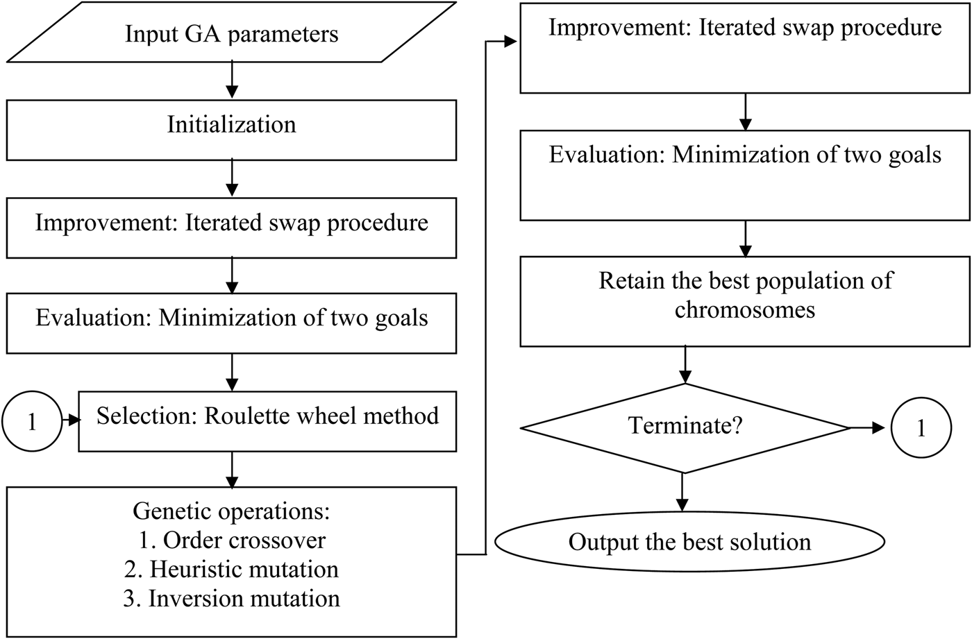
In order to solve this practical problem a GA is considered. John Holland proposed GAs in the 1960s for the first time. A PVRP can be regarded as a hard optimization problem. In order to enrich the capability of the proposed GA in this paper, it is hybridized with some other approaches. The GA developed in this paper benefits from a new approach toward acceptance criteria with a local search. Figure 3 shows the flowchart of HGA for the PVRP. HGA hybridizes an improved heuristic called the iterated swap procedure (ISP). Besides the ISP, it also hybridizes the saving method of Clarke and Wright (Reference Clarke and Wright1964) to generate a population of initial chromosomes. In addition, the authors use three genetic operators to make good new offspring.
The flowchart of the hybrid genetic algorithm. Reprinted from “A Novel Hybrid Genetic Algorithm to Solve the Make-to-Order Sequence-Dependent Flow-Shop Scheduling Problem,” by M. Mirabi, S.M.T. Fatemi, and F. Jolai, Reference Mirabi, Fatemi and Jolai2014, Journal of Industrial Engineering International 10(57), 4, Figure 1. Copyright 2014 by Springer. Reprinted with permission of the authors.
Here is a description of the procedure of the HGA. After the GA parameters, such as the iteration number, the population size (P size), the crossover rate, and the mutation rate, have been set, the HGA generates the initial chromosomes of the problem. After the predetermined number of initial chromosomes is generated (P size), the ISP is adopted to improve all chromosomes based on the evaluation function. The roulette wheel selection operation is applied to select some chromosomes for the genetic operations, including the order crossover, the heuristic mutation, and the inversion mutation. After a new chromosome is produced, its links are improved by the ISP. The fitness of the offspring is measured, and the offspring may become a member of the population if it has better quality than its parent. Therefore, the ISP applies two times: after initialization and after genetic operations, and every time a candidate chromosome after the ISP yields a better solution, it is replaced with the parent. These steps form iteration, and then the roulette wheel selection is performed again to start the next iteration. The HGA will not stop unless the predetermined number of iterations is conducted. Detailed explanations of the presented stages in Figure 3 are presented in the following subsections.
2.1.1. Initialization
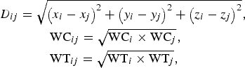
At this stage, a pool of initial solutions is extracted (P size). In each solution, customers are assigned to vehicles to take service (routing) and then the sequence of service in each route is determined (scheduling). The basis of the work in this section is the saving method in Clarke and Wright (Reference Clarke and Wright1964). Assume (x i, y i, z i) is the situation of customer i in the production hall (x-y-z volume); WCi is the waiting cost per time for customer i, and WTi is the waiting time during which the customer i is working without needing service. At first, for every two customers i and j the following parameters are calculated:
 $$\eqalign{& {D_{ij}} = \sqrt {{{\left({{x_i} - {x_j}} \right)}^2} + {{\left({{y_i} - {y_j}} \right)}^2} + {{\left({{z_i} - {z_j}} \right)}^2}}\comma \; \cr & \hskip 3.2pc {\rm W}{{\rm C}_{ij}} = \sqrt {{\rm W}{{\rm C}_i} \times {\rm W}{{\rm C}_j}} \comma \; \cr & \hskip 3.2pc {\rm W}{{\rm T}_{ij}} = \sqrt {{\rm W}{{\rm T}_i} \times {\rm W}{{\rm T}_j}} \comma \; }$$
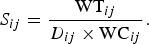
where D ij is the distance between customer i and customer j, WCij is the geometric mean of waiting costs of customer i and j, and WTij is the geometric mean of WTi and WTj. For each customer i and j, one heuristic index as S ij is defined as follows:
 $$S_{ij}=\displaystyle{{{\rm W}{{\rm T}_{ij}}} \over {{D_{ij}} \times {\rm W}{{\rm C}_{ij}}}}.$$
Based on the author's experience and the test problems, the geometric mean gains the best results at initialization. Algorithm 1 proposed an approach to gain n initial solutions.
Algorithm 1: Initialization
1. Number all vehicles from 1 to m.
2. Construct S ij for every two distinct customers (i and j can be varied from 1 to n, where n is the number of customers).
3. Sort S ij in descending order.
4. Allocate the largest S ij (implied two customers) to vehicle number 1, go to the next largest S ijthat i and j (or one of them if only one customer left) are not assigned before and allocate related customer(s) to vehicle number 2, and so on until the last vehicle. Then allocate the next S ij to vehicle number 1 again and continue this process until the least S ij.
5. For scheduling problem at each route, use the nearest neighborhood (NNH) algorithm. The principle of the NNH is to start with the first customer randomly. Then the next waiting customer is selected as close as possible to the previous one from those unselected customers to form the delivery sequence until all customers are selected. In addition, in the new added customer situation, we use NNH to form the sequence of service.
6. Extract the final result
7. For k = 2: P size
8. Randomly select two customer allocated in two distinct route
9. Interchange these two customers between two routes
10. Extract the final result
11. End for
12. Extract all P size results
By the S ij the author is going to allocate two customers with the least distance and geometric mean of waiting cost and also with the most geometric mean of working time to the same vehicle or route.
For customer scheduling in each route (sequence of getting service), NNH (Hemmelmayr et al., Reference Hemmelmayr, Doerner and Hartl2009) is used (algorithm 1, line 5). After line 6 of algorithm 1, there is only one solution for the problem but in genetics it needs a pool of initial solutions (P size). Interchange approach is performed to gain this pool (algorithm 1, lines 7–11). After this stage, we gain P size initial solutions.
To map each initial solution to genetic encoding (permutation encoding), we use path representation. For example, consider the parent of Figure 4. It means there are three vehicles and eight customers, and vehicle 1 starts from the depot, travels to customer 2, ends customer 4, and goes back to the depot, and so on.
A parent of pool solution.
In permutation encoding, every chromosome (represent as a solution) is a string of numbers, which represents number in a sequence. As can be seen in algorithm 1 (line 5), after each service, when new customer(s) is added to take service, the related vehicle updates its schedule by using NNH.
2.1.2. Improvement
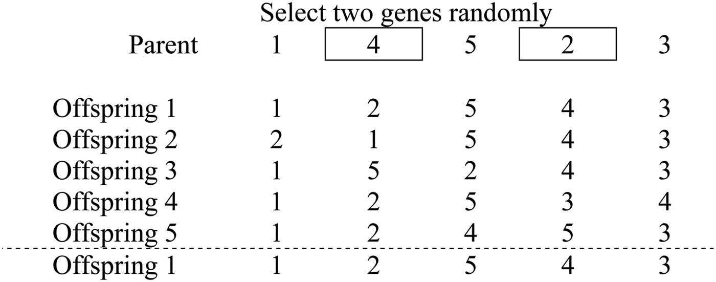
The 2-opt local search heuristic is generally used to improve the solutions of the hard optimization problems. However, it increases the computational time because every two swaps are examined. If a new solution generated is better than the original one, or parent, in terms of quality, it will replace and become the parent. All two swaps are examined again until there is no further improvement in the parent. To increase efficiency, the ISP (Ho & Ji, Reference Ho and Ji2003, Reference Ho and Ji2004) shown in Figure 5 is used to improve the links of each initial solution and each offspring generated by the three genetic operators. The principle of the ISP is similar to that of the 2-opt local search heuristic, except that some instead of all two swaps are examined. The procedure of the ISP is as follows:
Step 1. Select two genes randomly from a parent.
Step 2. Exchange the positions of the two genes to form an offspring.
Step 3. Swap the neighbors of the two genes to form four more offspring.
Step 4. Evaluate all offspring and find the best one.
Step 5. If the best offspring is better than the parent, replace the parent with the best offspring and go back to Step 1; otherwise, stop.
2.1.3. Evaluation
As mentioned before, the fitness function is minimizing total traveled distance (equivalent to traveling cost) at each depot and total waiting time (equivalent to waiting cost) of all customers to take service. Therefore for each solution h, objective function can defined as follows (h = 1, 2, … , P size):
 $$C\lpar h\rpar = {\rm min}\sum\nolimits_{i = 1}^n \!{\left({{\rm W}{{\rm C}_i} \times {t_i}} \right)} + \sum\nolimits_{k = 1}^m \!{\left({{\rm T}{{\rm C}_k} \times {d_k}} \right)} \comma \;$$
in which t i is the total waiting time of customer i in one complete time period (e.g., 8 h), where waiting time means the machine needs service and the vehicle could not do that; TCk is traveling cost per length of vehicle k; and d k is total traveling distance of vehicle k in one complete time period. Assuming 8 h as a complete time period is usually a good choice for a customer entering and leaving the system during the simulation especially in the textile industry cases considered in this research. In the presented approach, a customer with more working time and less waiting cost is expected wait more to take service.
2.1.4. Selection
The roulette wheel selection operation (Goldberg, Reference Goldberg1989) is adopted to choose some chromosomes to undergo genetic operations. The approach is based on an observation that a roulette wheel has a section allocated for each chromosome in the population, and the size of each section is proportional to the chromosome's fitness. The fitter the chromosome, the higher the probability of being selected. Although one chromosome has the highest fitness, there is no guarantee it will be selected. The only certain thing is that, on average, a chromosome will be chosen with the probability proportional to its fitness. Suppose the population size is P size, then the selection procedure is as follows:
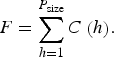
Step 1. Calculate the total fitness of the population:
 $$F = \sum\limits_{h = 1}^{P_{\rm size}} {C\left(h \right)} .$$
Step 2. Calculate the selection probability P h for each chromosome X h:
$${P_h} = \displaystyle{{F - {C_{{\rm max}}}\left(h \right)} \over {F \times \left({{P_{{\rm size}}} - 1} \right)}} \quad h=1\comma \; 2\comma \; .\;.\;.\; \comma \; P_{\rm size}.$$Step 3. Calculate the cumulative probability Q h for each chromosome X h:
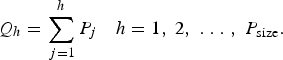
$${Q_h} = \sum\limits_{\,j = 1}^h {{P_j}} \quad h=1\comma \; 2\comma \; .\;.\;.\;\comma \; P_{\rm size}.$$Step 4. Generate a random number r in the range (0, 1).
Step 5. If Q h−1 < r ≤ Q h, then chromosome X h is selected.

2.1.5. Genetic operation
The genetic search progress is obtained by two essential genetic operations, including exploitation and exploration. Generally, the crossover operator exploits a better solution, while the mutation operator explores a wider search space. The genetic operators used in the algorithms for the PVRP are one crossover and two mutations, which are called the heuristic mutation and the inversion mutation, respectively.
The order crossover. The crossover operator adopted in the HGA is the classical order crossover (Gen & Cheng Reference Gen and Cheng1997), and two offspring will be generated at each time. The procedure of the order crossover operation is the following:
Step 1. Select a substring from the first parent randomly.
Step 2. Produce an offspring by copying the substring into the corresponding positions in the offspring.
Step 3. Delete those genes in the substring from the second parent. The resulting genes form a sequence.
Step 4. Place the genes into the unfilled positions of the offspring from left to right according to the resulting sequence of genes in Step 3 to produce an offspring, shown in Figure 6.
Step 5. Repeat Steps 1–4 to produce another offspring by exchanging the two parents.
The iterated swap procedure.
The order crossover operator. Reprinted from “A Novel Hybrid Genetic Algorithm to Solve the Make-to-Order Sequence-Dependent Flow-Shop Scheduling Problem,” by M. Mirabi, S.M.T. Fatemi, and F. Jolai, Reference Mirabi, Fatemi and Jolai2014, Journal of Industrial Engineering International 10(57), 6, Figure 4. Copyright 2014 by Springer. Reprinted with permission of the authors.
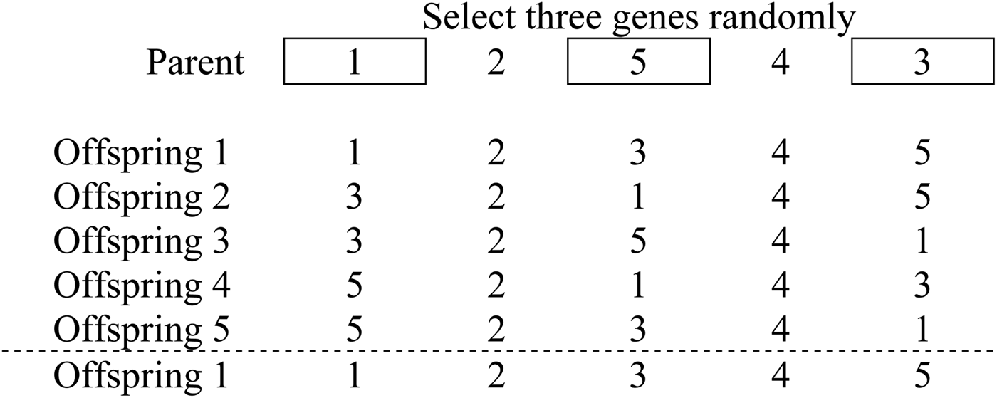
The heuristic mutation. A heuristic mutation (Gen & Cheng, Reference Gen and Cheng1997) is designed with the neighborhood technique to produce a better offspring. A set of chromosomes transformed from a parent by exchanging some genes is regarded as the neighborhood. Only the best one in the neighborhood is used as the offspring produced by the mutation. The purpose of the mutation operation is to promote diversity of the population, and it is necessary to use the heuristic mutation for the PVRP. The modification is that all neighbors generated are used as the offspring. The procedure of the heuristic mutation operation, shown in Figure 7, is taken as follows:
Step 1. Pick up three genes in a parent at random.
Step 2. Generate neighbors for all possible permutations of the selected genes, and all neighbors generated are regarded as the offspring.
The inversion mutation. The inversion operator (Gen & Cheng, Reference Gen and Cheng1997), shown in Figure 8, selects a substring from a parent and flips it to form an offspring. However, the inversion operator works with one chromosome only. It is similar to the heuristic mutation and thus lacks the interchange of characteristics between chromosomes. Therefore, the inversion operator is a mutation operation, which is used to increase the diversity of the population rather than to enhance the quality of the population.
The heuristic mutation operator. Reprinted from “A Novel Hybrid Genetic Algorithm to Solve the Make-to-Order Sequence-Dependent Flow-Shop Scheduling Problem,” by M. Mirabi, S.M.T. Fatemi, and F. Jolai, Reference Mirabi, Fatemi and Jolai2014, Journal of Industrial Engineering International 10(57), 6, Figure 5. Copyright 2014 by Springer. Reprinted with permission of the authors.
The inversion mutation operator. Reprinted from “A Novel Hybrid Genetic Algorithm to Solve the Make-to-Order Sequence-Dependent Flow-Shop Scheduling Problem,” by M. Mirabi, S.M.T. Fatemi, and F. Jolai, Reference Mirabi, Fatemi and Jolai2014, Journal of Industrial Engineering International 10(57), 6, Figure 6. Copyright 2014 by Springer. Reprinted with permission of the authors.
2.2. MDPVRP
We are interested to decompose this condition to PVRP condition and use the previous algorithm. Therefore, before scheduling decisions, grouping decisions must be made. It requires clustering a set of customers to be served by the same depot, that is, the grouping problem. It is clear that to allocate customers to depots, two major data are critical to determine the priority of allocation: working time and waiting cost. Each customer that has a higher waiting cost and less working time has a greater priority to allocate to the nearest depot. Grouping decision requires the steps of algorithm 2 (K is the number of customers):
Algorithm 2: Grouping decision ()
1. For each customer k, calculate PRk = WTk/WCk (k = 1, 2, … , K).
2. Sort PRk in ascending order.
3. For k = 1:K.
Assign the kth customer in the ascending list to the nearest depot.
4. End.
Here, PRk is the priority of customer k. If the nearest depot is not unique, the selection of depot and assignment to the customer is made arbitrarily. It is clear based on the above assignment each customer is assigned to the nearest vehicle, but another important factor in these problems is balancing the workload among depots (Pisinger & Ropke, Reference Pisinger and Ropke2007) To perform this we take the following steps:
5. Calculate the workload of each depot (work time per unit of time like day)
6. While balance of workload is not achieved
Go to the depot with the most loads
Take one customer with the least priority from customer assignment list
Put the customer in the customer list of depot with the least load
End
3. COMPUTATIONAL RESULTS
This section describes the computational tests that are used to evaluate and verify the effectiveness and efficiency of the proposed algorithm to find good quality results. For this purpose, the author tested the following methods:
• an asynchronous parallel metaheuristics (APM) by Drummond et al. (Reference Drummond, Ochi and Vianna2001)
• a variable neighborhood search (VNS) heuristic by Hemmelmayr et al. (Reference Hemmelmayr, Doerner and Hartl2009)
• an HGA proposed by Ho et al. (Reference Ho, Ho, Ji and Lau2008)
• the HGA proposed in this paper (HGA*)
It is noticeable that if, during vehicle traveling, some new customers are added as waiting customers for service, we encounter a new VRP, and an insertion procedure is used to find the route for all methods (Lim & Zhu, Reference Lim and Zhu2006). Two different classes of problems were used in the computational experiments: class 1: single depot problem; class 2: two depots problem. The parameters of the HGA for the problems are population size = 20, crossover rate = 0.5, and mutation rate = 0.2.
Service time and independent work time for each customer are random integers from Uniform distributions [10, 15] and [30, 60], respectively. Computational testing was conducted on some of test problems. The author randomly generated these problems because no suitable test exists for the VRP with considered features. Within the test, we varied two problem characteristics: number of vehicles and number of customers. Each problem is tested with one, three, and five vehicles and 20, 50, and 100 customers.
The standard approach in the experimental comparison of evolutionary algorithms is to repeat several runs on the same problem because of the stochastic nature of the algorithms. Therefore, for each problem instance 10 runs are done. As an example of the notation, consider the MD520 set of problems: it consists of 10 runs of problem instance with two depots, five vehicles, and 20 customers. Considering all configurations tested, we obtain a total of 150 runs of 15 problem instances.
One 8-h work cycle is taken into account. Each problem instance was solved using each method. The relative error (RE) for each method h is computed as follows:
 $${\rm RE}=\lpar M_h - {\rm BS}\rpar /{\rm BS}\comma \;$$
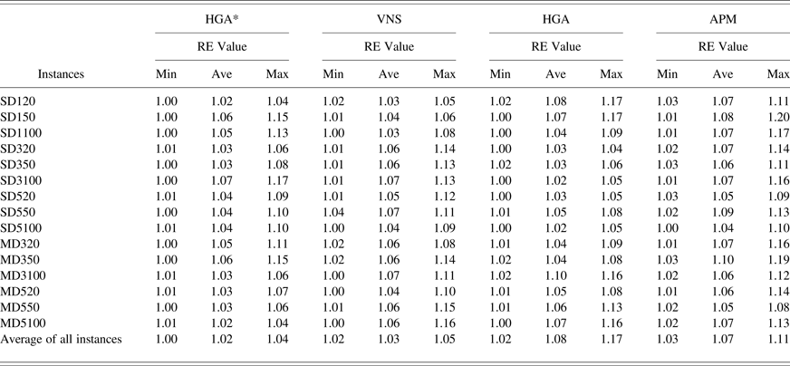
where M h is the solution for the method h and BS is the best solution among four methods. The average, minimum, and maximum RE values for two methods are shown in Table 1. All algorithms were coded by Matlab software and run on a PC that has a Pentium 2200-MHz processor, with 1024 MB of RAM.
RE values for computational test of four methods
Note: HGA, Hybrid genetic algorithm; VNS, variable neighborhood search; APM, asynchronous parallel metaheuristic; RE, relative error.
In addition, to have equal condition between methods, all algorithms are run 10 independent times with a stopping criterion based on an elapsed CPU time given by a × b/2 s, where a is the number of customers and b is the number of vehicles. This allows us to increase solution time as the number of customers a and the number of vehicles b grows.
Table 1 demonstrates that HGA* outperforms other algorithms based on RE index in most cases (its RE = 1 in most cases). In accordance with RE values, it is noticeable that HGA* and HGA are the two best methods among all. Therefore, it is interesting to have a detailed comparison between HGA* and HGA.
To cover this goal, the author tests the hypothesis that the differences has mean µ = 0. Specifically, we test the (null) hypothesis µ = 0 against the alternative µ > 0. It is assumed that the solution difference is a normal variable, and so we choose the significance level α = 0.05. If the hypothesis is true, the random variable
 $$T = \lpar {\bar X_1} - {\bar X_2}\rpar \!{/}\!\!\sqrt {\lpar S_1^2 /{n_1}\rpar + \lpar S_2^2 /{n_2}\rpar }$$
has a t distribution with
 $$\upsilon = {\lpar S_1^2 /{n_1} + S_2^2 /{n_2}\rpar ^2} \!{/} \!\!\bigg ( \displaystyle{{{{\lpar S_1^2 /{n_1}\rpar }^2}} \over {{n_1} - 1}} + \displaystyle{{{{\lpar S_2^2 /{n_2}\rpar }^2}} \over {{n_2} - 1}}\bigg)$$
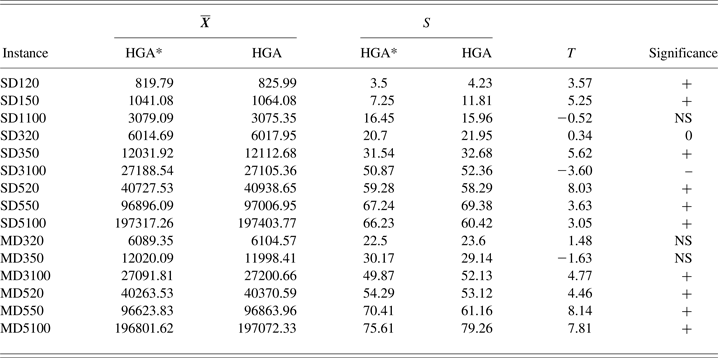
degrees of freedom. The critical value of c is obtained from the relation Prob(T > c) = α = 0.05. For example, the first entry in Table 2 corresponds to the sample size = n 1 = n 2 = 10, µ0 = 0, sample mean for HGA* and HGA are  ${{\bar X}_1} = 819.79$ and
 ${{\bar X}_2} = 825.99$, respectively. Sample standard deviation for HGA* and HGA are S 1 = 3.5 and S 2 = 4.23, respectively. Because t = 1.74 < T = 3.57, we conclude that the difference is statistically significant. Table 2 displays HGA* outperformed HGA in all cases except three, and 83% of differences are significant. In addition, Table 2 displays HGA outperformed HGA* in three cases and that one difference is significant.
Results of a T test to evaluate the significance of differences
Note: Each instance contains 10 independent tests.  $\overline X $, Average; S, standard deviation; HGA, hybrid genetic algorithm; +, HGA* is significantly better; –, HGA* is significantly worse; NS, no significant difference.
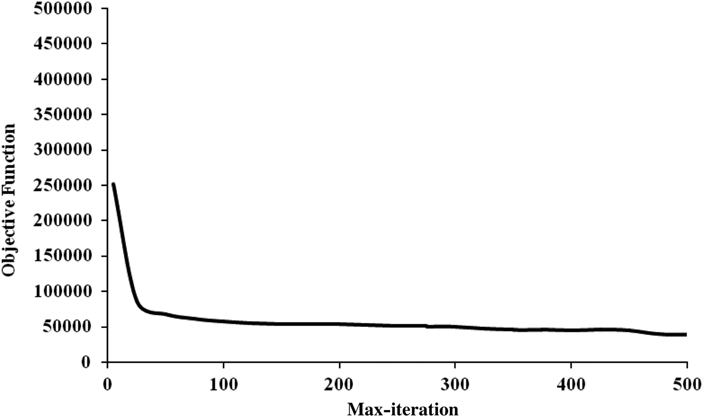
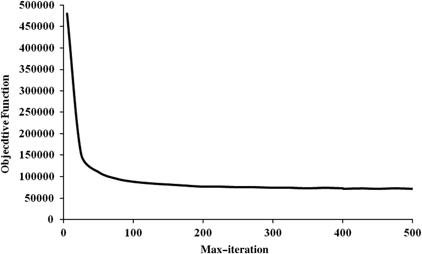
In our proposed algorithm, the initialization phase has a strong effect to accelerate the rate of HGA* convergence to as good final solution. To demonstrate this, the relationship between elapsed time and also the result of the final solution (objective function of best solution during optimization) is shown in two conditions: first using random generation to reach a pool of initial solutions and second with using the initialization phase to find a pool of initial solutions. Two convergent curves are drawn in Figures 9 and 10. To do this, instance SD3100 is selected.
Convergent curve for SD3100 with using random generation.
Convergent curve for SD3100 with using initialization phase.
These figures demonstrate the strong effect of the initial phase to reach the good final solution in a short time. As a result, HGA performed as a good approach to solve PVRP and MDPVRP in comparison to the recent approach in this area and also proposed that the initialization phase has a strong effect to reach the solution in a reasonable time.
4. CONCLUSIONS
This paper described one definition of PVRP for single and multidepots to conform to the wide ranges of real-world problems. The researcher has used two criteria that occur in real-world problems, namely, total traveled distance at each depot and total waiting time of all customers to take service. Distances are assumed Euclidean or straight line. In the presented problem, no vehicle can be idle when any customer is waiting for service. This is compatible with the real problems, especially in production systems when a machine is waiting for service or activity setting is made. Therefore, the minimum number of the required vehicles functions does not influence our problem. The problem is NP hard, and certainly exact methods are not usable. To solve the presented problem, one noble HGA is developed. The proposed HGA applies a modified approach to generate population of initial chromosomes and also to use an improved heuristic called the ISP for improving initial solutions. Computational experiments proved the compatibility of the proposed method compared to some strongest algorithms in this area.
Solving other branches of VRP, especially VRPTW and MDVRPTW, by GA and solving these problems by other strong metaheuristics like ant colony optimization, electromagnetism like algorithms, simulated annealing, and Tabu search can be suggested as interesting fields of research in the future.
Mohammad Mirabi teaches in the Department of Industrial Engineering at Ayatollah Haeri University of Meybod.