1. Introduction
This paper studies the stability properties of the two-dimensional incompressible magnetohydrodynamic (MHD) system with only vertical dissipation, given by
 \begin{equation}
\left\{
\begin{aligned}
&\partial_{t}U+U\cdot\nabla U-\nu\partial_{yy} U+\nabla P=B\cdot\nabla B, \\[4pt]
&\partial_{t}B+U\cdot\nabla B-\mu\partial_{yy} B=B\cdot\nabla U,\\[4pt]
&{\rm div}\, U={\rm div}\, B=0,
\end{aligned}
\right.
\end{equation}
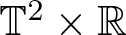
posed on the periodic strip  $\Omega:=\mathbb{T}\times \mathbb{R}$, where
 $U=(U_1,U_2)$ and
 $B=(B_1,B_2)$ denote the velocity and magnetic field, respectively, and
 $P$ the pressure. The positive constants
 $\nu$ and
 $\mu$ represent the viscosity and magnetic diffusivity coefficients.
Anisotropic dissipation arises naturally in many physical systems, ranging from atmospheric circulation to plasma dynamics (see, e.g., [Reference Cao, Li and Titi4, Reference Cao and Wu5, Reference Elgindi and Widmayer13, Reference Ji, Tian and Wu17, Reference Paicu and Zhang31, Reference Paicu and Zhang32, Reference Xu and Zhang41]). In particular, geophysical fluid dynamics provides a canonical example: turbulent diffusivity in the vertical direction is often orders of magnitude larger than in the horizontal direction. The absence of full dissipation renders the classical energy method insufficient, requiring refined tools such as frequency-space decompositions and anisotropic energy estimates. This intermediate regime, situated between full dissipation and nondissipative dynamics, plays a crucial role in understanding incomplete turbulence observed in natural systems.
Since Reynolds’s pioneering experiments [Reference Reynolds36], understanding the transition from laminar to turbulent flows has remained a central challenge in fluid dynamics. Kelvin’s classical analysis in 1887 [Reference Kelvin19] already revealed that laminar flows may persist at large Reynolds numbers if the initial perturbation is sufficiently small. A more extensive physical discussion can be found in [Reference Chandrasekhar6, Reference Davidson9, Reference Hughes and Tobias16]. Over the past decade, remarkable progress has been made towards rigorously establishing stability thresholds for Couette flows in various fluid models, giving rise to a rapidly growing literature (see, e.g., [Reference Bedrossian, Germain and Masmoudi1–Reference Bedrossian, Vicol and Wang3, Reference Chen, Li, Wei and Zhang7, Reference Chen, Wei and Zhang8, Reference Deng, Wu and Zhang10–Reference Dolce, Knobel and Zillinger12, Reference Huang, Sun and Xu14, Reference Huang, Sun and Xu15, Reference Jin, Ren and Wei18, Reference Knobel and Zillinger22–Reference Niu, Wu, Wu and Xu30, Reference Rao, Zhang and Zi33–Reference Ren and Wei35, Reference Wang and Zhang37–Reference Wu, Wu and Xu40, Reference Zeng, Zhang and Zi42, Reference Zhao and Zi43]).
It is clear that the Couette flow
 \begin{equation*}
\tilde{U}=(y,0), \qquad \tilde{B}=(0,0)
\end{equation*}
is a stationary solution of (1.1). Our aim is to analyse the nonlinear stability of this flow within the framework of 2D MHD with vertical dissipation. Introducing perturbations
 \begin{equation*}
u=U-\tilde{U}, \qquad \mathfrak{B}=B-\tilde{B},
\end{equation*}
the dynamics of 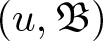 $(u,\mathfrak{B})$ is governed by
 \begin{equation}
\left\{
\begin{aligned}
&\partial_{t}u+y\partial_{x}u-\nu\partial_{yy}u+(u_{2},0)^{t}=-\nabla p-u\cdot\nabla u+\mathfrak{B}\cdot \nabla \mathfrak{B},\\[4pt]
&\partial_{t}\mathfrak{B}+y\partial_{x}\mathfrak{B}-\mu\partial_{yy}\mathfrak{B}-(\mathfrak{B}_{2},0)^{t}=-u\cdot\nabla \mathfrak{B}+\mathfrak{B}\cdot\nabla u,\\[4pt]
&{\rm div}\, u={\rm div}\, \mathfrak{B}=0,\\[4pt]
&(u,\mathfrak{B})(t,x,y)|_{t=0}=(u_{0},\mathfrak{B}_{0})(x,y),
\end{aligned}
\right.
\end{equation}
where the pressure is determined by
 \begin{equation*}
p=(-\Delta)^{-1}\!\left(2\partial_{x}u_{2}\right)+(-\Delta)^{-1}\nabla\cdot(u\cdot\nabla u-\mathfrak{B}\cdot\nabla \mathfrak{B}).
\end{equation*}
To simplify the equations in (1.2), we introduce the vorticity  $\omega=\nabla\times u$ and the magnetic stream function
 $\phi$ defined by
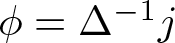 $\phi=\Delta^{-1}j$ with current density
 $j=\nabla\times \mathfrak{B}$. In terms of
 $(\omega,\phi)$, the system takes the form
 \begin{equation}
\left\{
\begin{aligned}
&\partial_{t}\omega+y\partial_{x}\omega-\nu\partial_{yy}\omega=-u\cdot\nabla\omega+\mathfrak{B}\cdot\nabla\Delta\phi,\\[4pt]
&\partial_{t}\phi+y\partial_{x}\phi-\mu\partial_{yy}\phi=-u\cdot\nabla\phi,\\[4pt]
&u=-\nabla^{\perp}(-\Delta)^{-1}\omega, \qquad \mathfrak{B}=\nabla^{\perp}\phi.
\end{aligned}
\right.
\end{equation}
The focus of this work is precisely on the vertical dissipation regime, where dissipation acts exclusively in the  $y$-direction. Compared to prior works, our analysis does not rely on coordinate transformations and instead exploits the special structure of the magnetic stream function. One key point here is that the equation for the magnetic stream function
 $\phi$ does not have any bad linear terms, as that of the equation for the magnetic field, which contains
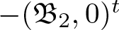 $-(\mathfrak{B}_2, 0)^t$. This approach allows us to uncover new stability mechanisms specific to the anisotropically dissipative MHD system.
We remark that the absence of horizontal dissipative mechanisms in system (1.3) precludes the derivation of stability estimates through standard energy methods. Motivated by the work of Deng, Wu, and Zhang [Reference Deng, Wu and Zhang10] on the 2D Boussinesq equations, we utilize the appropriate Fourier multiplier technique to capture the enhanced dissipation and inviscid damping associated with the structure 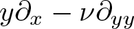 $y\partial_{x}-\nu\partial_{yy}$. This approach yields a gain of
 $1/3$ of a horizontal derivative while simultaneously establishing a zero-order dissipation estimate represented via a Riesz transform-type operator for the nonzero Fourier modes.
The Fourier multiplier operator 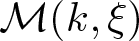 $\mathcal{M}(k,\xi)$ is defined as
 \begin{equation}
\mathcal{M}=\mathcal{M}_{1}+\mathcal{M}_{2}+1,
\end{equation}
where  $\mathcal{M}_{1}$ and
 $\mathcal{M}_{2}$ are given by
 \begin{equation}
\begin{aligned}
&\mathcal{M}_{1}(k,\xi)=\varphi\!\left(\varpi^{\frac{1}{3}}|k|^{-\frac{1}{3}}\operatorname{sgn}(k)\xi\right), \qquad &k\neq0,\\
&\mathcal{M}_{2}(k,\xi)=\arctan\!\left(\tfrac{\xi}{k}\right)+\tfrac{\pi}{2}, \qquad &k\neq0,\\
&\mathcal{M}_{1}(0,\xi)=\mathcal{M}_{2}(0,\xi)=0, \qquad &k=0,
\end{aligned}
\end{equation}
with  $\varpi=\min\{\nu,\mu\}$. Here,
 $\varphi$ is a smooth, real-valued, non-decreasing function,
 $\varphi\in C^{\infty}(\mathbb{R})$, satisfying
 \begin{equation*}
0\leqslant \varphi(x)\leqslant 1, \qquad 0\leqslant \varphi'(x)\leqslant \tfrac{1}{4}, \quad x\in\mathbb{R}, \qquad
\varphi'(x)=\tfrac{1}{4}, \quad x\in[-1,1].
\end{equation*}
The operator  $\mathcal{M}$ is thus a self-adjoint Fourier multiplier on
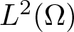 $L^2(\Omega)$, and one readily checks that
 \begin{equation*}
1 \leqslant \mathcal{M} \leqslant 2+\pi.
\end{equation*}
From (1.4)–(1.5), we obtain the key coercivity estimate
 \begin{equation}
\begin{aligned}
k\partial_{\xi}\mathcal{M}+\nu\xi^{2}\;\geqslant\;
(k\partial_{\xi}\mathcal{M}_{1}+\varpi\xi^{2})+k\partial_{\xi}\mathcal{M}_{2}
\;\geqslant\;\tfrac{1}{4}\varpi^{\frac{1}{3}}|k|^{\frac{2}{3}}+\frac{k^{2}}{k^{2}+\xi^{2}},
\end{aligned}
\end{equation}
valid for all  $k\neq 0$,
 $\nu \gt 0$, and
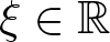 $\xi\in \mathbb{R}$. As a representative case, consider the vorticity equation for
 $\omega$. We deduce
 \begin{equation}
\langle (y\partial_x-\nu \partial_{yy})\omega, \mathcal{M}\omega\rangle
\;\geqslant\;\tfrac{1}{4}\,\varpi^{\frac{1}{3}}\|\,|D_x|^{\frac{1}{3}}\omega\|_{L^2}^2
+\|\,|D_{x}|(-\Delta)^{-\frac12}\omega^{\neq}\|_{L^2}^2.
\end{equation}
Consequently, the following dissipation inequality holds for the linearized system:
 \begin{equation*}
\frac{d}{dt}\|\sqrt{\mathcal{M}}\omega\|_{L^{2}}^{2}
+\nu\|\partial_{y}\omega\|_{L^{2}}^{2}
+\tfrac{1}{4}\varpi^{\frac{1}{3}}\|\,|D_{x}|^{\frac{1}{3}}\omega\|_{L^{2}}^{2}
+\|\,|D_{x}|(-\Delta)^{-\frac{1}{2}}\omega^{\neq}\|_{L^{2}}^{2}\;\leqslant\;0.
\end{equation*}
To state our main result precisely, we first introduce several notations. For  $t \geqslant 0$ and
 $b \in \mathbb{R}$, we define
 \begin{equation*}
\mathcal{M}^{b}_{t}:=\sqrt{\mathcal{M}}\,\Lambda^{b}_{t},
\qquad
\mathcal{M}^{b}_{t}(k,\xi):=\sqrt{\mathcal{M}(k,\xi)}\,\Lambda^{b}_{t}(k,\xi),
\end{equation*}
where the time-dependent elliptic operator  $\Lambda^{b}_{t}$ is given for any
 $b\in \mathbb{R}$ and
 $t \geqslant 0$ by
 \begin{equation*}
\Lambda^{b}_{t}:=\big(1-\partial^{2}_{x}-(\partial_{y}+t\partial_{x})^{2}\big)^{\frac{b}{2}},
\end{equation*}
or equivalently, in Fourier space,
 \begin{equation*}
\Lambda^{b}_{t}(k,\xi):=\big(1+k^{2}+(\xi+tk)^{2}\big)^{\frac{b}{2}}.
\end{equation*}
Here, the Fourier transform is defined by
 \begin{equation*}
\hat{f}(k,\xi):=\int_{\mathbb{R}}e^{-i\xi y}\int_{\mathbb{T}}e^{-ikx}f(x,y)\,dx\,dy.
\end{equation*}
The operator  $\Lambda^{b}_{t}$ was first introduced in [Reference Deng, Wu and Zhang10]. For each fixed
 $t \geqslant 0$, it behaves like the standard nonhomogeneous fractional differential operator
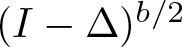 $(I-\Delta)^{b/2}$. A key property of
 $\Lambda^{b}_{t}$ is its commutation with the transport operator
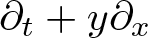 $\partial_t + y \partial_x$, namely,
 \begin{equation*}
\Lambda^{b}_{t} (\partial_t + y \partial_x) = (\partial_t + y \partial_x)\Lambda^{b}_{t}.
\end{equation*}
This commutation allows Sobolev norms to be estimated without breaking the intrinsic transport structure of the equations, and plays a crucial role in our analysis.
We also introduce notations for horizontal averages and oscillatory modes. For any function 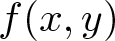 $f(x,y)$, we write
 \begin{equation*}
f=\bar{f}+f^{\neq},
\end{equation*}
where
 \begin{equation*}
\bar{f}:=\int_{\mathbb{T}} f(x,y)\,dx,
\qquad
f^{\neq}:=f-\bar{f}.
\end{equation*}
The fractional derivative in the  $x$-variable is defined in Fourier space by
 \begin{equation*}
\widehat{|D_x|^\gamma f}(k, \xi) = |k|^\gamma \hat f(k, \xi).
\end{equation*}
Throughout this paper,  $C$ denotes a positive constant independent of
 $\nu$, whose value may vary from line to line. We also adopt the shorthand
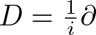 $D=\tfrac{1}{i}\partial$ and
 \begin{equation*}
\|(f,g)\|_{L^{2}}:=\|f\|_{L^{2}}+\|g\|_{L^{2}}.
\end{equation*}
These notations will be used throughout the paper to formulate our stability estimates and state the main theorems.
Our main result is stated as follows:
Theorem 1.1. Assume  $b \gt 1$,
 $\varpi= \min\{\nu, \mu\}$,
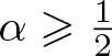 $\alpha\geqslant \frac{1}{2}$,
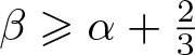 $\beta\geqslant \alpha+\frac{2}{3}$,
 $\frac{5}{6}\leqslant\gamma\leqslant 2\alpha-\frac{1}{6}$ and
 $\nabla\cdot u_{0}=\nabla\cdot \mathfrak{B}_{0}=0$. Let
 $\omega_0$,
 $j_0$, and
 $\phi_0$ denote the initial vorticity, current density, and magnetic stream function, respectively. Then, there exists a sufficiently small positive constant
 $\varepsilon$, such that if the initial data
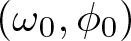 $(\omega_{0},\phi_{0})$ satisfy
 \begin{equation*}
\|(\omega_{0},j_{0})\|_{H^{b}} \leqslant \varepsilon \varpi^{\alpha},\quad \||D_{x}|^{\frac{2}{3}}\phi_{0}\|_{H^{b}} \leqslant \varepsilon \varpi^{\beta},\quad \|\partial_{y}\bar{\phi}_{0}\|_{H^{b}} \leqslant \varepsilon \varpi^{\gamma},
\end{equation*}
then the Cauchy problem (1.3) admits a unique global solution 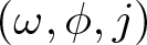 $(\omega,\phi,j)$ satisfying
 \begin{equation*}
\begin{aligned}
&\|\Lambda^{b}_{t}(\omega,j)\|_{L^{\infty}L^{2}} +\varpi^{\frac{1}{2}}\|\Lambda^{b}_{t}\partial_{y}(\omega,j)\|_{L^{2}L^{2}}+\varpi^{\frac{1}{6}}\|\Lambda^{b}_{t}\vert D_{x}\vert^{\frac{1}{3}}(\omega,j)\|_{L^{2}L^{2}}\\
&\ \ \ \ \ \ \ \ \ \ \ \ \ \ \ \ \ \ \ \ \ \ \ \ \ \ \ \ \ \ \ \ \ \ \ \ \ \ \ +\|\Lambda^{b}_{t}|D_{x}|(-\Delta)^{-\frac{1}{2}}(\omega,j)\|_{L^{2}L^{2}}\leqslant C\varepsilon \varpi^{\alpha},\\
&\|\Lambda^{b}_{t}|D_{x}|^{\frac{2}{3}}\phi\|_{L^{\infty}L^{2}} +\mu^{\frac{1}{2}}\|\Lambda^{b}_{t}\partial_{y}|D_{x}|^{\frac{2}{3}}\phi\|_{L^{2}L^{2}}+\varpi^{\frac{1}{6}}\|\Lambda^{b}_{t}\vert D_{x}\vert^{\frac{1}{3}}|D_{x}|^{\frac{2}{3}}\phi\|_{L^{2}L^{2}}\\
& \ \ \ \ \ \ \ \ \ \ \ \ \ \ \ \ \ \ \ \ \ \ \ \ \ \ \ \ \ \ \ \ \ \ \ \ \ \ \ +\|\Lambda^{b}_{t}|D_{x}|(-\Delta)^{-\frac{1}{2}}|D_{x}|^{\frac{2}{3}}\phi\|_{L^{2}L^{2}}\leqslant C\varepsilon \varpi^{\beta},\\
&\|\Lambda^{b}_{t}\partial_{y}\bar{\phi}\|_{L^{\infty}L^{2}} +\mu^{\frac{1}{2}}\|\Lambda^{b}_{t}\partial_{yy}\bar{\phi}\|_{L^{2}L^{2}}\leqslant C\varepsilon \varpi^{\gamma},
\end{aligned}
\end{equation*}
where  $C \gt 0$ is independent of
 $\nu,\mu,\alpha,\beta,\gamma$, and
 $\varepsilon$.
We add a remark on the restrictions imposed on 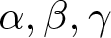 $\alpha,\beta,\gamma$, and on their sharpness.
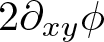
Remark 1.1. The restrictions on 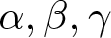 $\alpha,\beta,\gamma$ arise from the intrinsic anisotropic scaling of the linearized MHD–Couette system with vertical dissipation. The current equation (1.9) contains the linear stretching term
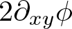 $2\partial_{xy}\phi$, whose control through vertical diffusion produces an unavoidable
 $\mu^{-1}$ loss (see (1.11) and (2.38)). On the other hand, the transport–diffusion operator
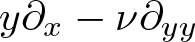 $y\partial_x-\nu\partial_{yy}$ yields a gain of
 $1/3$ horizontal derivative via enhanced dissipation (see (1.6)–(1.7)). These two linear effects determine the scaling of the nonlinear energy inequalities (2.6). Requiring that each nonlinear term carry a nonnegative power of
 $\varpi=\min\{\nu,\mu\}$ leads precisely to
 \begin{equation*}
\alpha\geqslant \tfrac12,\qquad
\beta\geqslant \alpha+\tfrac23,\qquad
\tfrac56\le \gamma\le 2\alpha-\tfrac16 .
\end{equation*}
Hence the exponents in Theorem 1.1 are consistent with the anisotropic scaling of the problem and are essentially sharp within the present energy framework. Any substantial relaxation would require a mechanism compensating the  $\mu^{-1}$ stretching loss or improving the
 $1/3$ enhanced dissipation gain.
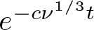
We also remark that the explicit enhanced dissipation decay 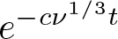 $e^{-c\nu^{1/3}t}$ can be incorporated into the estimates of Theorem 1.1.
Remark 1.2. The explicit enhanced dissipation rate 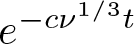 $e^{-c\nu^{1/3}t}$ can be obtained within the framework of Theorem 1.1. In particular, for the nonzero Fourier modes we have
 \begin{equation}
\|\Lambda^{b}_{t}(\omega,j)\|_{L^{2}}
\le C\varepsilon \varpi^{\alpha}e^{-c\nu^{1/3}t},\qquad
\|\Lambda^{b}_{t}|D_{x}|^{2/3}\phi\|_{L^{2}}
\le C\varepsilon \varpi^{\beta}e^{-c\nu^{1/3}t},
\end{equation}
where  $c \gt 0$ is a constant independent of
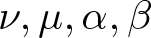 $\nu,\mu,\alpha,\beta$, and
 $\varepsilon$. These bounds follow by incorporating the time weight
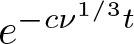 $e^{-c\nu^{1/3}t}$ into the energy functionals. The enhanced dissipation rate
 $e^{-c\nu^{1/3}t}$ is already implicit in the linear coercivity estimate of the multiplier
 $\mathcal{M}$. More precisely, estimate (1.7) yields
 \begin{equation*}
\frac{d}{dt}\|\sqrt{\mathcal{M}}\,\omega\|_{L^2}^2
+ c\nu^{1/3}\||D_x|^{1/3}\omega\|_{L^2}^2 \le 0,
\end{equation*}
for some  $c \gt 0$. Since
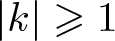 $|k|\geqslant1$ on the nonzero Fourier modes, this implies
 \begin{equation*}
\frac{d}{dt}\|\omega_{\neq}\|_{L^2}^2
+ c\nu^{1/3}\|\omega_{\neq}\|_{L^2}^2 \le 0,
\end{equation*}
and hence
 \begin{equation*}
\|\omega_{\neq}(t)\|_{L^2}
\le e^{-c\nu^{1/3}t}\|\omega_{\neq}(0)\|_{L^2}.
\end{equation*}
A special consequence of Theorem 1.1 is the following corollary.
Corollary 1.2. Assume the same conditions as in Theorem 1.1. If the initial value  $\phi_{0}$ satisfies
 \begin{equation*}
\|\phi_{0}\|_{H^{b}} \leqslant \varpi^{\lambda} \quad \text{for} \quad \lambda\geqslant 0,
\end{equation*}
then the system admits a unique global solution  $\phi$ satisfying
 \begin{align*}
\begin{aligned}
&\|\Lambda^{b}_{t}\phi\|_{L^{\infty}L^{2}} +\mu\|\Lambda^{b}_{t}\partial_{y}\phi\|_{L^{2}L^{2}}+\varpi^{\frac{1}{3}}\|\Lambda^{b}_{t}\vert D_{x}\vert^{\frac{1}{3}}\phi\|_{L^{2}L^{2}} \nonumber\\
& \quad +\|\Lambda^{b}_{t}|D_{x}|(-\Delta)^{-\frac{1}{2}}\phi\|_{L^{2}L^{2}}\leqslant C\varpi^{\lambda}.
\end{aligned}
\end{align*}
We now turn to the main analytical difficulties underlying Theorem 1.1. The foremost obstacle arises from the nonlinear term 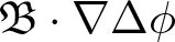 $\mathfrak{B}\cdot \nabla \Delta \phi$ in the vorticity equation of system (1.3). Controlling this term requires sharp estimates on higher-order derivatives of the magnetic stream function
 $\phi$. Since the current density is defined by
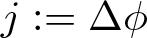 $j:=\Delta \phi$, we derive the governing equation
 \begin{equation}
\begin{aligned}
\partial_{t}j+y\partial_{x}j -\mu\partial_{yy} j+2\partial_{xy}\phi=-u\cdot \nabla j+\mathfrak{B}\cdot \nabla \omega-Q(\nabla u,\nabla \mathfrak{B}),
\end{aligned}
\end{equation}
where the quadratic form is given by
 \begin{equation}
\begin{aligned}
Q(\nabla u,\nabla \mathfrak{B}):=2\partial_{x}u_{1}(\partial_{x}\mathfrak{B}_{2}+\partial_{y}\mathfrak{B}_{1})-2\partial_{x}\mathfrak{B}_{1}(\partial_{x}u_{2}+\partial_{y}u_{1}).
\end{aligned}
\end{equation}
The symmetry between vorticity  $\omega$ and current density
 $j$ plays a crucial role: it enables us to balance the nonlinear advective terms
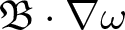 $\mathfrak{B}\cdot\nabla \omega$ and
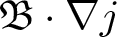 $\mathfrak{B}\cdot\nabla j$, thereby recovering stability.
A further challenge stems from the additional linear term 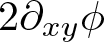 $2\partial_{xy}\phi$ appearing in (1.9), which complicates the energy estimates. To overcome this, we construct auxiliary energy functionals. Specifically,
 \begin{equation}
\begin{aligned}
\langle -\Lambda^{b}_{t}2\partial_{xy}\phi, \mathcal{M}\Lambda^{b}_{t}j\rangle\leqslant C\mu^{-1}\|\Lambda^{b}_{t}\partial_{x}\phi\|_{L^{2}}^{2}+\epsilon\mu \|\Lambda^{b}_{t}\partial_{y}j\|_{L^{2}}^{2}.
\end{aligned}
\end{equation}
The  $\mu^{-1}$ factor in the leading term reveals the necessity of refined bounds on
 $\|\Lambda^{b}_{t}|D_{x}|\phi\|_{L^{2}L^{2}}$. To achieve this, we incorporate fractional horizontal derivatives of
 $\phi$ into the energy functional.
This refinement introduces yet another difficulty: nonlinear terms now require control of  $\partial_{y}\bar{\phi}$. In fact,
 \begin{equation}
\begin{aligned}
&\langle \Lambda^{b}_{t}(\vert D_{x}\vert^{\frac{2}{3}}u\cdot \nabla \phi), \mathcal{M}\Lambda^{b}_{t}\vert D_{x}\vert^{\frac{2}{3}}\phi\rangle\\
=&\langle \mathcal{M}^{b}_{t}(\vert D_{x}\vert^{\frac{2}{3}}u\cdot \nabla \phi^{\neq}), \mathcal{M}^{b}_{t}\vert D_{x}\vert^{\frac{2}{3}}\phi\rangle+\langle \mathcal{M}^{b}_{t}(\vert D_{x}\vert^{\frac{2}{3}}u\cdot \nabla \bar{\phi}), \mathcal{M}^{b}_{t}\vert D_{x}\vert^{\frac{2}{3}}\phi\rangle\\
\leqslant &C\|\Lambda^{b}_{t}\vert D_{x}\vert^{\frac{2}{3}}\phi\|_{L^{2}}(\|\Lambda^{b}_{t}\vert D_{x}\vert^{\frac{2}{3}}u_{2}\|_{L^{2}}\|\Lambda^{b}_{t}\partial_{y}\phi^{\neq}\|_{L^{2}}+\|\Lambda^{b}_{t}\vert D_{x}\vert^{\frac{2}{3}}u_{1}\|_{L^{2}}\|\Lambda^{b}_{t}\vert D_{x}\vert\phi\|_{L^{2}})\\
&\ \ +C\|\Lambda^{b}_{t}\vert D_{x}\vert^{\frac{2}{3}}\phi\|_{L^{2}}\|\Lambda^{b}_{t}\vert D_{x}\vert^{\frac{2}{3}}u_{2}\|_{L^{2}}\|\Lambda^{b}_{t}\partial_{y}\bar{\phi}\|_{L^{2}}.
\end{aligned}
\end{equation}
Thus, as indicated in (1.12), the control of nonlinear interactions necessitates an auxiliary functional tied to 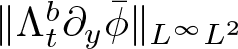 $\|\Lambda^{b}_{t}\partial_{y}\bar{\phi}\|_{L^{\infty}L^{2}}$.
We finally remark that one may alternatively analyse the vorticity–current system  $(\omega,j)$ in sheared coordinates and treat the linear stretch term
 $2\partial_{xy}\phi$ using Fourier multipliers. We instead work with the magnetic stream function
 $\phi$, whose equation possesses a more favourable linear structure and commutes with the transport operator
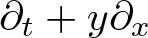 $\partial_t+y\partial_x$. Moreover, the nonlocal relation
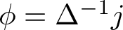 $\phi=\Delta^{-1}j$ is handled more directly in the present anisotropic (vertical-only) dissipation framework, particularly for the zero mode.
Recent years have seen substantial progress on stability and transition thresholds for the 2D MHD equations near Couette flow. In the presence of a constant background magnetic field, Dolce [Reference Dolce11] established the Sobolev stability threshold and enhanced dissipation for the 2D MHD equations using symmetric variables. Sobolev stability thresholds for partially dissipative MHD near Couette were obtained by Knobel and Zillinger [Reference Knobel and Zillinger22], who analysed regimes with anisotropic magnetic dissipation. Nonlinear stability and enhanced dissipation in Sobolev spaces for the 2D MHD system with uniform magnetic field were further proved by Jin, Ren, and Wei [Reference Knobel18]. Knobel and Zillinger [Reference Knobel and Zillinger21] analysed nonlinear resonance mechanisms for the 2D MHD equations with magnetic dissipation near a combination of Couette flow and constant background magnetic field. They constructed explicit global low-frequency solutions and showed that the linearized dynamics around these states exhibit high-frequency resonant interactions leading to echo chains, which produce Gevrey-class norm inflation and infinite-time blow-up in Sobolev regularity. More recently, Knobel [Reference Knobel20] developed a unified framework for Sobolev stability thresholds of 2D dissipative fluid equations, including the MHD equations near Couette flow, based on the suppression of nonlinear fluid-echo interactions. Complementary to these stability results, Dolce, Knobel, and Zillinger [Reference Dolce, Knobel and Zillinger12] investigated instability mechanisms for the viscous, non-resistive 2D MHD equations near Couette flow, proving large-norm inflation of the current despite viscosity. Their analysis also employs the magnetic stream-function formulation. All of the above works rely on sheared or moving coordinate transformations adapted to the Couette flow, whereas the present analysis avoids coordinate changes and instead exploits the special structure of the magnetic stream-function formulation.
The remainder of this paper is organized as follows. Section 2 establishes a key lemma for the a priori estimates, introduces several energy functionals, and applies a bootstrap argument to prove Theorem 1.1 through three propositions. Section 3 is devoted to the proof of Corollary 1.2.
2. Proof of Theorem 1.1
In this section, we first review several useful estimates in Sobolev spaces. We then proceed to establish the nonlinear stability of system (1.3) using the Fourier multiplier method. In the course of the analysis, we exploit the special structure of the magnetic stream function to overcome difficulties arising from the nonlinear terms in the velocity and magnetic field equations. Finally, we employ a bootstrap argument to close the estimates by constructing appropriate energy functionals.
2.1. An important lemma
We begin with the following lemma.
Lemma 2.1. ([Reference Deng, Wu and Zhang10])
For any  $b\in \mathbb{R}$, it holds that
 \begin{equation*}\Lambda^{b}_{t}(\partial_{t}+y\partial_{x})=(\partial_{t}+y\partial_{x})\Lambda^{b}_{t}.\end{equation*}
Furthermore, for any  $b \gt 0$,
 \begin{equation*}\| \Lambda^{b}_{t}(fg)\|_{L^{2}}\leqslant \| f\|_{L^{\infty}}\| \Lambda^{b}_{t}g\|_{L^{2}}+\| g\|_{L^{\infty}}\| \Lambda^{b}_{t}f\|_{L^{2}}.\end{equation*}
In addition, for any  $b \gt 1$,
 \begin{equation*}\| f\|_{L^{\infty}(\Omega)}\leqslant C\| \hat{f}\|_{L^{1}(\Omega)}\leqslant C\| \Lambda^{b}_{t}f(t)\|_{L^{2}(\Omega)}.\end{equation*}
2.2. Proof of Theorem 1.1
Our main focus is the stability problem for system (1.3), with the key task being the derivation of global uniform a priori estimates for the solutions. To this end, we first introduce the following energy functional:
 \begin{equation}
\begin{aligned}
E_{1}(t) := \sup_{t \gt 0} \Big\{& \|\Lambda^{b}_{t}(\omega,j)\|_{L^{\infty}L^{2}}
+ \varpi^{\frac{1}{2}}\|\Lambda^{b}_{t}\partial_{y}(\omega,j)\|_{L^{2}L^{2}}
+ \varpi^{\frac{1}{6}}\|\Lambda^{b}_{t}|D_{x}|^{\frac{1}{3}}(\omega,j)\|_{L^{2}L^{2}} \\
& + \|\Lambda^{b}_{t}|D_{x}|(-\Delta)^{-\frac{1}{2}}(\omega,j)\|_{L^{2}L^{2}} \Big\},
\end{aligned}
\end{equation}
with the initial energy
 \begin{equation*}
E_{1}(0) := \|(\omega_{0}, j_{0})\|_{H^{b}}.
\end{equation*}
The intermediate energy functional is defined by
 \begin{equation}
\begin{aligned}
E_{2}(t) := \sup_{t \gt 0} \Big\{& \|\Lambda^{b}_{t}|D_{x}|^{\frac{2}{3}}\phi\|_{L^{\infty}L^{2}}
+ \mu^{\frac{1}{2}}\|\Lambda^{b}_{t}\partial_{y}|D_{x}|^{\frac{2}{3}}\phi\|_{L^{2}L^{2}}
+ \varpi^{\frac{1}{6}}\|\Lambda^{b}_{t}|D_{x}|\phi\|_{L^{2}L^{2}} \\
& + \|\Lambda^{b}_{t}|D_{x}|^{\frac{5}{3}}(-\Delta)^{-\frac{1}{2}}\phi\|_{L^{2}L^{2}} \Big\},
\end{aligned}
\end{equation}
with
 \begin{equation*}
E_{2}(0) := \||D_{x}|^{\frac{2}{3}}\phi_{0}\|_{H^{b}}.
\end{equation*}
The zero-mode energy functional of  $\phi$ is given by
 \begin{equation}
E_{3}(t) := \sup_{t \gt 0} \Big\{\|\Lambda^{b}_{t}\partial_{y}\bar{\phi}\|_{L^{\infty}L^{2}}
+ \mu^{\frac{1}{2}}\|\Lambda^{b}_{t}\partial_{yy}\bar{\phi}\|_{L^{2}L^{2}} \Big\},
\end{equation}
with
 \begin{equation*}
E_{3}(0) := \|\partial_{y}\bar{\phi}_{0}\|_{H^{b}}.
\end{equation*}
Through detailed derivations and a bootstrap argument, the desired estimates are established via the following three propositions.
Proposition 2.1. There exists a constant  $C \gt 0$ such that, for all
 $t \gt 0$,
 \begin{equation*}
E_{1}^{2}(t) \leqslant E_{1}^{2}(0) + C \varpi^{-\frac{1}{2}} E_{1}^{3}(t) + C \mu^{-\frac{4}{3}} E_{2}^{2}(t).
\end{equation*}
Proposition 2.2. There exists a constant  $C \gt 0$ such that, for all
 $t \gt 0$,
 \begin{equation*}
E_{2}^{2}(t) \leqslant E_{2}^{2}(0) + C \varpi^{-\frac{1}{2}} E_{1}(t) E_{2}^{2}(t) + C \varpi^{-\frac{1}{6}} E_{1}(t) E_{2}(t) E_{3}(t).
\end{equation*}
Proposition 2.3. There exists a constant  $C \gt 0$ such that, for all
 $t \gt 0$,
 \begin{equation*}
E_{3}^{2}(t) \leqslant E_{3}^{2}(0) + C \varpi^{-\frac{1}{6}} E_{1}^{2}(t) E_{3}(t).
\end{equation*}
Proof of Theorem 1.1. Assume that the initial data 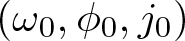 $(\omega_{0}, \phi_{0}, j_{0})$ satisfy
 \begin{equation}
\|(\omega_{0}, j_{0})\|_{H^{b}} \leqslant \varepsilon \varpi^{\alpha}, \quad
\||D_{x}|^{\frac{2}{3}}\phi_{0}\|_{H^{b}} \leqslant \varepsilon \varpi^{\beta}, \quad
\|\partial_{y}\bar{\phi}_{0}\|_{H^{b}} \leqslant \varepsilon \varpi^{\gamma},
\end{equation}
where  $\varepsilon \gt 0$ is sufficiently small and
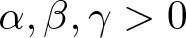 $\alpha, \beta, \gamma \gt 0$. To apply the bootstrap argument, we make the ansatz that
 \begin{equation}
\begin{aligned}
E_{1}(t)\leqslant C_{1}\varepsilon \varpi^{\alpha},\quad E_{2}(t)\leqslant C_{2} \varepsilon \varpi^{\beta}, \quad E_{3}(t)\leqslant C_{3}\varepsilon \varpi^{\gamma},
\end{aligned}
\end{equation}
Inserting the initial condition (2.4) and the bootstrap ansatz (2.5) into Propositions 2.1–2.3, we obtain
 \begin{equation}
\begin{aligned}
E_{1}^{2}(t) &\leqslant \varepsilon^{2} \varpi^{2\alpha} + C C_{1}^{3} \varepsilon^{3} \varpi^{3\alpha - \frac{1}{2}} + C C_{2}^{2} \varepsilon^{2} \varpi^{2\beta} \mu^{-\frac{4}{3}},\\
E_{2}^{2}(t) &\leqslant \varepsilon^{2} \varpi^{2\beta} + C C_{1} C_{2}^{2} \varepsilon^{3} \varpi^{\alpha + 2\beta - \frac{1}{2}} + C C_{1} C_{2} C_{3} \varepsilon^{3} \varpi^{\alpha + \beta + \gamma - \frac{1}{6}},\\
E_{3}^{2}(t) &\leqslant \varepsilon^{2} \varpi^{2\gamma} + C C_{1}^{2} C_{3} \varepsilon^{3} \varpi^{2\alpha + \gamma - \frac{1}{6}}.
\end{aligned}
\end{equation}
Here, we choose parameters satisfying
 \begin{equation}
\begin{aligned}
\alpha \geqslant \frac{1}{2}, \quad \beta \geqslant \alpha + \frac{2}{3}, \quad \frac{5}{6} \leqslant \gamma \leqslant 2\alpha - \frac{1}{6},
\end{aligned}
\end{equation}
and take  $\varepsilon$ sufficiently small such that
 \begin{equation*}
\varepsilon \leqslant \min\Bigg\{
\frac{\frac{1}{4}C_{1}^{2} - 1 - C C_{2}^{2}}{C C_{1}^{3}}, \quad
\frac{\frac{1}{4}C_{2}^{2} - 1}{C C_{1} C_{2} (C_{2} + C_{3})}, \quad
\frac{\frac{1}{4}C_{3}^{2} - 1}{C C_{1}^{2} C_{3}}
\Bigg\}.
\end{equation*}
Under these choices, we deduce
 \begin{equation}
E_{1}(t) \leqslant \frac{C_{1}}{2} \varepsilon \varpi^{\alpha}, \quad
E_{2}(t) \leqslant \frac{C_{2}}{2} \varepsilon \varpi^{\beta}, \quad
E_{3}(t) \leqslant \frac{C_{3}}{2} \varepsilon \varpi^{\gamma}.
\end{equation}
It follows from the bootstrap argument that (2.5) holds. This completes the proof of Theorem 1.1.
2.3. Proof of Proposition 2.1
This section is devoted to the proof of Proposition 2.1.
Proof of Proposition 2.1
First, we apply the operator  $\Lambda^{b}_{t}$ to
 $(1.3)_{1}$ and, using Lemma 2.1, take the
 $L^{2}$ inner product of the resulting equation with
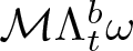 $\mathcal{M}\Lambda^{b}_{t}\omega$. This gives
 \begin{equation}
\begin{aligned}
\big\langle \partial_{t}\Lambda^{b}_{t}\omega + y\partial_{x}\Lambda^{b}_{t}\omega - \nu \partial_{yy}\Lambda^{b}_{t}\omega, \mathcal{M} \Lambda^{b}_{t}\omega \big\rangle
= \big\langle \Lambda^{b}_{t}(-u\cdot \nabla \omega + \mathfrak{B}\cdot \nabla \Delta\phi), \mathcal{M} \Lambda^{b}_{t}\omega \big\rangle.
\end{aligned}
\end{equation}
To handle the nonlinear term 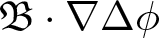 $\mathfrak{B} \cdot \nabla \Delta\phi$, we require higher-order derivative estimates for
 $\phi$. Applying
 $\Delta$ to
 $(1.3)_{2}$ yields system (1.9) with the quadratic form (1.10). Similarly, applying
 $\Lambda^{b}_{t}$ to (1.9) and taking the
 $L^{2}$ inner product with
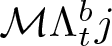 $\mathcal{M}\Lambda^{b}_{t}j$ gives
 \begin{equation}
\begin{aligned}
&\langle \partial_{t}\Lambda^{b}_{t}j+y\partial_{x}\Lambda^{b}_{t}j-\mu\partial_{yy} \Lambda^{b}_{t}j+2\partial_{xy}\Lambda^{b}_{t}\phi, \mathcal{M} \Lambda^{b}_{t}j\rangle \\
&\ \ \ \ =\langle \Lambda^{b}_{t}(-u\cdot \nabla j+\mathfrak{B}\cdot \nabla \omega-Q(\nabla u,\nabla \mathfrak{B})), \mathcal{M} \Lambda^{b}_{t}j\rangle.
\end{aligned}
\end{equation}
According to the properties of multiplier  $\mathcal{M} $ and (1.7), we get that
 \begin{equation}
\begin{aligned}
&LHS~~ of~~ (2.9)+ (2.10)\\
&\geqslant \frac{1}{2}\frac{d}{dt}\|\mathcal{M}^{b}_{t}(\omega,j)\|_{L^{2}}^{2}+\frac{1}{2}\mu\|\mathcal{M}^{b}_{t}\partial_{y}j\|_{L^{2}}^{2}+\frac{1}{8}\varpi^{\frac{1}{3}}\|\mathcal{M}^{b}_{t}\vert D_{x}\vert^{\frac{1}{3}}(\omega,j)\|_{L^{2}}^{2} \\
&\ \ \ \ +\frac{1}{2}\nu\|\mathcal{M}^{b}_{t}\partial_{y}\omega\|_{L^{2}}^{2}+\frac{1}{2}\|\mathcal{M}^{b}_{t}|D_{x}|(-\Delta)^{-\frac{1}{2}}(\omega,j)\|_{L^{2}}^{2}+\langle 2\partial_{xy}\Lambda^{b}_{t}\phi, \mathcal{M} \Lambda^{b}_{t}j\rangle.
\end{aligned}
\end{equation}
Then we estimate the nonlinear terms. Combining (2.9) and (2.10), we have
 \begin{equation}
\begin{aligned}
&\ \ \ \ RHS~~ of~~ (2.9)+ (2.10)\\
&=-\underbrace{\langle \Lambda^{b}_{t}(u\cdot \nabla \omega), \mathcal{M}\Lambda^{b}_{t}\omega\rangle}_{I_{1}}-\underbrace{\langle\Lambda^{b}_{t}Q(\nabla u,\nabla \mathfrak{B}), \mathcal{M}\Lambda^{b}_{t}j\rangle}_{I_{2}}-\underbrace{\langle \Lambda^{b}_{t}(u\cdot \nabla j), \mathcal{M}\Lambda^{b}_{t}j\rangle}_{I_{3}}\\
&\ \ \ \ +\underbrace{\langle \Lambda^{b}_{t}(\mathfrak{B}\cdot \nabla j), \mathcal{M}\Lambda^{b}_{t}\omega\rangle+\langle \Lambda^{b}_{t}(\mathfrak{B}\cdot \nabla \omega), \mathcal{M}\Lambda^{b}_{t}j\rangle}_{I_{4}}.
\end{aligned}
\end{equation}
 $\bullet$ Estimate of
 $I_{1}$. By
 ${\rm div}\,u=0$ and
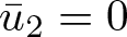 $\bar{u}_{2}=0$, we arrive at
 \begin{equation*}
\begin{aligned}
I_{1}&=\langle \mathcal{M}^{b}_{t}(u\cdot \nabla \omega)-u\cdot \nabla(\mathcal{M}^{b}_{t}\omega), \mathcal{M}^{b}_{t}\omega\rangle\\
&=\langle \mathcal{M}^{b}_{t}(\bar{u}_{1}\partial_{x} \omega)-\bar{u}_{1}\partial_{x} (\mathcal{M}^{b}_{t}\omega), \mathcal{M}^{b}_{t}\omega\rangle+\langle \mathcal{M}^{b}_{t}(u_{1}^{\neq}\partial_{x} \omega)-u_{1}^{\neq}\partial_{x} (\mathcal{M}^{b}_{t}\omega), \mathcal{M}^{b}_{t}\omega\rangle\\
&\ \ \ \ +\langle \mathcal{M}^{b}_{t}(u_{2}^{\neq}\partial_{y} \omega)-u_{2}^{\neq}\partial_{y} (\mathcal{M}^{b}_{t}\omega), \mathcal{M}^{b}_{t}\omega\rangle\\
&:=I_{11}+I_{12}+I_{13}.
\end{aligned}
\end{equation*}
The estimate of  $I_{11}$ is given. By Plancherel’s formula, we get
 \begin{equation*}
\begin{aligned}
I_{11}
&:=\sum_{k\neq0}\iint(\mathcal{M}^{b}_{t}(k,\xi)-\mathcal{M}^{b}_{t}(k,\xi-\eta))\hat{u}_{1}(0,\eta)\cdot ik\hat{\omega}(k,\xi-\eta)\cdot\mathcal{M}^{b}_{t}(k,\xi)\overline{\hat{\omega}(k,\xi)}d\xi d\eta.
\end{aligned}
\end{equation*}
By the differential mean-value theorem, there holds
 \begin{equation*}
\begin{aligned}
&|\mathcal{M}^{b}_{t}(k,\xi)-\mathcal{M}^{b}_{t}(k,\xi-\eta)|\leqslant \int^{1}_{0}|\partial_{\xi}\mathcal{M}^{b}_{t}(k,\xi-s\eta)||\eta|ds\\
&\ \ \ \ \leqslant C|\eta|(\varpi^{\frac{1}{3}}|k|^{-\frac{1}{3}}+\frac{1}{(k^{2}+\xi^{2})^{\frac{1}{2}}}+\frac{1}{(k^{2}+(\xi-\eta)^{2})^{\frac{1}{2}}})(\Lambda^{b}_{t}(0,\xi)+\Lambda^{b}_{t}(k,\xi-\eta)),
\end{aligned}
\end{equation*}
where using the facts that
 \begin{equation*}
\begin{aligned}
\Lambda^{b}_{t}(k,\xi-s\eta)\leqslant \Lambda^{b}_{t}(0,\xi)+\Lambda^{b}_{t}(k,\xi-\eta)
\end{aligned}
\end{equation*}
and
 \begin{equation*}
\frac{1}{(k^{2}+(\xi-s\eta)^{2})^{\frac{1}{2}}}\leqslant \frac{2}{|k|+|\xi-s\eta|}\leqslant
\left\{
\begin{aligned}
\frac{2}{|k|+|\xi-\eta|},\quad for~~\xi\eta \gt 0,\\
\frac{2}{|k|+|\xi|},\quad for ~~\xi\eta \lt 0.
\end{aligned}
\right.
\end{equation*}
It holds that
 \begin{equation*}
\begin{aligned}
I_{11}
\leqslant C\sum_{k\neq 0}\iint(&\varpi^{\frac{1}{3}}|k|^{\frac{2}{3}}+\frac{|k|}{(k^{2}+\xi^{2})^{\frac{1}{2}}}+\frac{|k|}{(k^{2}+(\xi-\eta)^{2})^{\frac{1}{2}}})(\Lambda^{b}_{t}(0,\xi)+\Lambda^{b}_{t}(k,\xi-\eta))\\
&\times|\hat{\omega}(0,\eta)|| \hat{\omega}(k,\xi-\eta)||\mathcal{M}^{b}_{t}(k,\xi)\overline{\hat{\omega}(k,\xi)}|d\xi d\eta.
\end{aligned}
\end{equation*}
Hence, by Young’s convolution inequality, we obtain
 \begin{equation}
\begin{aligned}
I_{11}
\leqslant C(\varpi^{\frac{1}{3}}\|\Lambda^{b}_{t}\bar{\omega}\|_{L^{2}}\|\Lambda^{b}_{t}|D_{x}|^{\frac{1}{3}}\omega\|_{L^{2}}^{2}+\|\Lambda^{b}_{t}\bar{\omega}\|_{L^{2}}\|\Lambda^{b}_{t}|D_{x}|(-\Delta)^{-\frac{1}{2}}\omega\|_{L^{2}}\|\Lambda^{b}_{t}\omega^{\neq}\|_{L^{2}}).
\end{aligned}
\end{equation}
Now we estimate  $I_{12}$. By Plancherel’s formula, we derive
 \begin{align*}
I_{12} &:=\sum_{k,l}\iint(\mathcal{M}^{b}_{t}(k,\xi)-\mathcal{M}^{b}_{t}(l,\eta))\hat{u}_{1}^{\neq}(k-l,\xi-\eta)\\
&\quad \cdot il\hat{\omega}(l,\eta)\cdot\mathcal{M}^{b}_{t}(k,\xi)\overline{\hat{\omega}(k,\xi)}d\xi d\eta.
\end{align*}
Then dividing the frequency space into the following two parts:
 \begin{equation*}
\begin{aligned}
& A_{1}=\{(k,l)\in \mathbb{Z}^{2}: |k-l|\geqslant\frac{|l|}{2}~~ or ~~\min(|k|,|l|)\leqslant\varpi^{-\frac{1}{2}}\}, \\
& A_{2}=\{(k,l)\in \mathbb{Z}^{2}: |k-l| \lt \frac{|l|}{2} ~~and~~ \min(|k|,|l|) \gt \varpi^{-\frac{1}{2}}\},
\end{aligned}
\end{equation*}
this can be referred to [Reference Wei and Zhang39]. For the first case, one has
 \begin{equation*}|l|\leqslant2(|k-l|+\varpi^{-\frac{1}{6}}|l|^{\frac{1}{3}}|k|^{\frac{1}{3}}). \end{equation*}
Thereby,
 \begin{equation*}
\begin{aligned}
I_{121}
\leqslant C\sum_{k,l\in A_{1}}\iint(&\Lambda^{b}_{t}(l,\eta)+\Lambda^{b}_{t}(k-l,\xi-\eta))(|k-l|+\varpi^{-\frac{1}{6}}|l|^{\frac{1}{3}}|k|^{\frac{1}{3}})\\
&\times|\hat{u}_{1}^{\neq}(k-l,\xi-\eta)||\hat{\omega}^{\neq}(l,\eta)||\mathcal{M}^{b}_{t}(k,\xi)\overline{\hat{\omega}(k,\xi)}|d\xi d\eta.
\end{aligned}
\end{equation*}
By Lemma 2.1, we have
 \begin{equation}
\begin{aligned}
I_{121}
&\leqslant C(\|\Lambda^{b}_{t}\partial_{x}u_{1}\|_{L^{2}}\|\Lambda^{b}_{t}\omega^{\neq}\|_{L^{2}}\|\Lambda^{b}_{t}\omega\|_{L^{2}}+\varpi^{-\frac{1}{6}}\|\Lambda^{b}_{t}u_{1}^{\neq}\|_{L^{2}}\|\Lambda^{b}_{t}|D_{x}|^{\frac{1}{3}}\omega\|_{L^{2}}^{2}).
\end{aligned}
\end{equation}
For the second case, by Taylor’s formula, we get
 \begin{equation*}
\begin{aligned}
&|\mathcal{M}^{b}_{t}(k,\xi)-\mathcal{M}^{b}_{t}(l,\eta)|\\
& \leqslant\int^{1}_{0}|\partial_{\xi}\mathcal{M}^{b}_{t}(k,\eta+s(\xi-\eta))||\xi-\eta|ds+\int^{1}_{0}|\partial_{k}\mathcal{M}^{b}_{t}(l+s(k-l),\eta)||k-l|ds.
\end{aligned}
\end{equation*}
According to the definition of  $\mathcal{M}$, a direct computation gives
 \begin{equation*}|\partial_{\xi}\mathcal{M}^{b}_{t}(k,\xi)|\leqslant C(\varpi^{\frac{1}{3}}|k|^{-\frac{1}{3}}+|k|^{-1})\Lambda^{b}_{t}(k,\xi)\leqslant C\varpi^{\frac{1}{3}}|k|^{-\frac{1}{3}}\Lambda^{b}_{t}(k,\xi),\end{equation*}
 \begin{equation*} |\partial_{k}\mathcal{M}^{b}_{t}(k,\xi)|\leqslant C(\varpi^{\frac{1}{3}}|k|^{-\frac{4}{3}}|\xi|+|k|^{-1})\Lambda^{b}_{t}(k,\xi)\leqslant C(\varpi^{\frac{1}{2}}|\xi|+1)|k|^{-1}\Lambda^{b}_{t}(k,\xi).\end{equation*}
Then we have
 \begin{equation*}
\begin{aligned}
I_{122}
\leqslant C\sum_{k,l\in A_{2}}\iint(&\Lambda^{b}_{t}(l,\eta)+\Lambda^{b}_{t}(k-l,\xi-\eta))(\varpi^{\frac{1}{3}}|k|^{-\frac{1}{3}}|l|+1+\varpi^{\frac{1}{2}}|\eta|)\\
&\times|\hat{\omega}^{\neq}(k-l,\xi-\eta)||\hat{\omega}^{\neq}(l,\eta)||\mathcal{M}^{b}_{t}(k,\xi)\overline{\hat{\omega}(k,\xi)}|d\xi d\eta\\
\leqslant C\sum_{k,l\in A_{2}}\iint(&\Lambda^{b}_{t}(l,\eta)+\Lambda^{b}_{t}(k-l,\xi-\eta))(\varpi^{\frac{1}{3}}|k|^{\frac{1}{3}}|l|^{\frac{1}{3}}+\varpi^{\frac{2}{3}}|k|^{\frac{1}{3}}|\eta|)\\
&\times|\hat{\omega}^{\neq}(k-l,\xi-\eta)||\hat{\omega}^{\neq}(l,\eta)||\mathcal{M}^{b}_{t}(k,\xi)\overline{\hat{\omega}(k,\xi)}|d\xi d\eta.
\end{aligned}
\end{equation*}
By Lemma 2.1, it holds that
 \begin{equation}
\begin{aligned}
I_{122}\leqslant C(\varpi^{\frac{1}{3}}\|\Lambda^{b}_{t}\omega\|_{L^{2}}\|\Lambda^{b}_{t}|D_{x}|^{\frac{1}{3}}\omega\|_{L^{2}}^{2}+\varpi^{\frac{2}{3}}\|\Lambda^{b}_{t}\omega\|_{L^{2}}\|\Lambda^{b}_{t}|D_{x}|^{\frac{1}{3}}\omega\|_{L^{2}}\|\Lambda^{b}_{t}\partial_{y}\omega\|_{L^{2}}) .
\end{aligned}
\end{equation}
Hence, combining (2.14) and (2.15) yields
 \begin{equation}
\begin{aligned}
I_{12}
\leqslant& C\|\Lambda^{b}_{t}\omega\|_{L^{2}}(\varpi^{-\frac{1}{6}}\|\Lambda^{b}_{t}|D_{x}|^{\frac{1}{3}}\omega\|_{L^{2}}^{2}+\varpi^{\frac{2}{3}}\|\Lambda^{b}_{t}|D_{x}|^{\frac{1}{3}}\omega\|_{L^{2}}\|\Lambda^{b}_{t}\partial_{y}\omega\|_{L^{2}}) .
\end{aligned}
\end{equation}
Next, estimate  $I_{13}$. By Plancherel’s formula, we derive
 \begin{equation*}
\begin{aligned}
I_{13}
:=\sum_{k,l}\iint(&\mathcal{M}^{b}_{t}(k,\xi)-\mathcal{M}^{b}_{t}(k-l,\xi-\eta))\hat{u}_{2}^{\neq}(l,\eta)\cdot i(\xi-\eta)\hat{\omega}(k-l,\xi-\eta)\\
&\times\mathcal{M}^{b}_{t}(k,\xi)\overline{\hat{\omega}(k,\xi)}d\xi d\eta.
\end{aligned}
\end{equation*}
By Lemma 2.1 and the boundedness of multiplier  $\mathcal{M}$, we deduce
 \begin{equation}
\begin{aligned}
I_{13}
&\leqslant C\|\Lambda^{b}_{t}u_{2}^{\neq}\|_{L^{2}}\|\Lambda^{b}_{t}\partial_{y}\omega\|_{L^{2}}\|\Lambda^{b}_{t}\omega\|_{L^{2}}\\
&\leqslant C\|\Lambda^{b}_{t}|D_{x}|(-\Delta)^{-\frac{1}{2}}\omega^{\neq}\|_{L^{2}}\|\Lambda^{b}_{t}\partial_{y}\omega\|_{L^{2}}\|\Lambda^{b}_{t}\omega\|_{L^{2}}.
\end{aligned}
\end{equation}
Combining (2.13), (2.16), and (2.17), we have
 \begin{equation}
\begin{aligned}
I_{1}
&\leqslant C\|\Lambda^{b}_{t}\omega\|_{L^{2}}\|\Lambda^{b}_{t}|D_{x}|(-\Delta)^{-\frac{1}{2}}\omega\|_{L^{2}}(\|\Lambda^{b}_{t}|D_{x}|^{\frac{1}{3}}\omega^{\neq}\|_{L^{2}}+\|\Lambda^{b}_{t}\partial_{y}\omega\|_{L^{2}})\\
&\ \ \ \ +C\|\Lambda^{b}_{t}\omega\|_{L^{2}}\|\Lambda^{b}_{t}|D_{x}|^{\frac{1}{3}}\omega\|_{L^{2}}(\varpi^{-\frac{1}{6}}\|\Lambda^{b}_{t}|D_{x}|^{\frac{1}{3}}\omega\|_{L^{2}}+\varpi^{\frac{2}{3}}\|\Lambda^{b}_{t}\partial_{y}\omega\|_{L^{2}}).
\end{aligned}
\end{equation}
 $\bullet$ Estimate of
 $I_{2}$.
From (1.10), there holds that
 \begin{equation*}
\begin{aligned}
I_{2}&=\langle \mathcal{M}^{b}_{t}(2\partial_{x}u_{1}(\partial_{x}\mathfrak{B}_{2}+\partial_{y}\mathfrak{B}_{1})-2\partial_{x}\mathfrak{B}_{1}(\partial_{x}u_{2}+\partial_{y}u_{1})), \mathcal{M}^{b}_{t}j\rangle\\
&=\langle\mathcal{M}^{b}_{t}( 2\partial_{x}u_{1}(2\partial_{x}\mathfrak{B}_{2}-j)-2\partial_{x}\mathfrak{B}_{1}(2\partial_{x}u_{2}-\omega)), \mathcal{M}^{b}_{t}j\rangle\\
&\leqslant C\|\Lambda^{b}_{t}j\|_{L^{2}}(\|\Lambda^{b}_{t}\partial_{x}u_{1}\|_{L^{2}}\|\Lambda^{b}_{t}\partial_{x}\mathfrak{B}_{2}\|_{L^{2}}+\|\Lambda^{b}_{t}\partial_{x}\mathfrak{B}_{1}\|_{L^{2}}\|\Lambda^{b}_{t}\partial_{x}u_{2}\|_{L^{2}})\\
&\ \ \ \ \ \ \ \ + \underbrace{\langle\mathcal{M}^{b}_{t}( 2\partial_{x}u_{1}\cdot(-j)+2\partial_{x}\mathfrak{B}_{1}\cdot\omega), \mathcal{M}^{b}_{t}j\rangle}_{I_{21}}.
\end{aligned}
\end{equation*}
To estimate  $I_{21}$, by Plancherel’s formula, we arrive at
 \begin{equation*}
\begin{aligned}
I_{21}
&=-2\sum_{k,l}\iint \mathcal{M}^{b}_{t}(k,\xi) \cdot il\hat{u}_{1}^{\neq}(l,\eta)\hat{j}(k-l,\xi-\eta)\cdot \mathcal{M}^{b}_{t}(k,\xi)\overline{\hat{j}(k,\xi)}d\xi d\eta\\
&\ \ \ \ \ \ +2\sum_{k,l}\iint \mathcal{M}^{b}_{t}(k,\xi)\cdot il\hat{\mathfrak{B}}_{1}^{\neq}(l,\eta)\hat{\omega}(k-l,\xi-\eta)\cdot \mathcal{M}^{b}_{t}(k,\xi)\overline{\hat{j}(k,\xi)}d\xi d\eta.
\end{aligned}
\end{equation*}
Due to the facts that  $|l|^{\frac{1}{3}}\leqslant |k-l|^{\frac{1}{3}}+ |k|^{\frac{1}{3}}$ and
 $\Lambda^{b}_{t}(k,\xi)\leqslant \Lambda^{b}_{t}(l,\eta)+\Lambda^{b}_{t}(k-l,\xi-\eta)$, it yields that
 \begin{equation*}
\begin{aligned}
|I_{21}| &\leqslant C\sum_{k,l}\iint |l|^{\frac{2}{3}}(|k-l|^{\frac{1}{3}}+ |k|^{\frac{1}{3}})(|\hat{u}_{1}^{\neq}(l,\eta)| |\hat{j}(k-l,\xi-\eta)|+ |\hat{\mathfrak{B}}_{1}^{\neq}(l,\eta)| |\\
&\quad \hat{\omega}(k-l,\xi-\eta)|)\times (\Lambda^{b}_{t}(l,\eta)+\Lambda^{b}_{t}(k-l,\xi-\eta)) \Lambda^{b}_{t}(k,\xi)|\hat{j}(k,\xi)|d\xi d\eta\\
&\leqslant C\|\Lambda^{b}_{t}|D_{x}|^{\frac{2}{3}}(u_{1}^{\neq},\mathfrak{B}_{1}^{\neq})\|_{L^{2}} \|\Lambda^{b}_{t}|D_{x}|^{\frac{1}{3}}(\omega,j)\|_{L^{2}}\|\Lambda^{b}_{t}(\omega,j)\|_{L^{2}}\\
&\leqslant C\|\Lambda^{b}_{t}D_{x}(-\Delta)^{-\frac{1}{2}}(\omega,j)\|_{L^{2}} \|\Lambda^{b}_{t}|D_{x}|^{\frac{1}{3}}(\omega,j)\|_{L^{2}}\|\Lambda^{b}_{t}(\omega,j)\|_{L^{2}}.
\end{aligned}
\end{equation*}
Thus, it holds
 \begin{equation}
\begin{aligned}
|I_{2}|
&\leqslant C\|\Lambda^{b}_{t}(\omega,j)\|_{L^{2}}(\|\Lambda^{b}_{t}D_{x}(-\Delta)^{-\frac{1}{2}}(\omega,j)\|_{L^{2}}^{2}+\|\Lambda^{b}_{t}|D_{x}|^{\frac{1}{3}}(\omega,j)\|_{L^{2}}^{2}).
\end{aligned}
\end{equation}
 $\bullet$ Estimate of
 $I_{3}$. By
 ${\rm div}\,u=0$ and
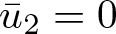 $\bar{u}_{2}=0$, we have
 \begin{equation*}
\begin{aligned}
I_{3}&=\langle \mathcal{M}^{b}_{t}(u\cdot \nabla j)-u\cdot \nabla(\mathcal{M}^{b}_{t}j), \mathcal{M}^{b}_{t}j\rangle\\
&=\langle \mathcal{M}^{b}_{t}(\bar{u}_{1}\partial_{x}j)-\bar{u}_{1}\partial_{x} (\mathcal{M}^{b}_{t}j), \mathcal{M}^{b}_{t}j\rangle+\langle \mathcal{M}^{b}_{t}(u_{1}^{\neq}\partial_{x} j)-u_{1}^{\neq}\partial_{x} (\mathcal{M}^{b}_{t}j), \mathcal{M}^{b}_{t}j\rangle\\
&\ \ \ \ +\langle \mathcal{M}^{b}_{t}(u_{2}^{\neq}\partial_{y} j)-u_{2}^{\neq}\partial_{y} (\mathcal{M}^{b}_{t}j), \mathcal{M}^{b}_{t}j\rangle\\
&:=I_{31}+I_{32}+I_{33}.
\end{aligned}
\end{equation*}
To estimate  $I_{31}$, by Plancherel’s formula, we get
 \begin{equation*}
\begin{aligned}
I_{31}
:=\sum_{k\neq0}\iint(\mathcal{M}^{b}_{t}(k,\xi)-\mathcal{M}^{b}_{t}(k,\xi-\eta))\hat{u}_{1}(0,\eta)\cdot ik&\hat{j}(k,\xi-\eta) \mathcal{M}^{b}_{t}(k,\xi)\overline{\hat{j}(k,\xi)}d\xi d\eta.
\end{aligned}
\end{equation*}
By the differential mean-value theorem, there holds that
 \begin{equation*}
\begin{aligned}
I_{31}
\leqslant C\sum_{k\neq 0}\iint(&\varpi^{\frac{1}{3}}|k|^{\frac{2}{3}}+\frac{|k|}{(k^{2}+\xi^{2})^{\frac{1}{2}}}+\frac{|k|}{(k^{2}+(\xi-\eta)^{2})^{\frac{1}{2}}})(\Lambda^{b}_{t}(0,\xi)+\Lambda^{b}_{t}(k,\xi-\eta))\\
&\times|\hat{\omega}(0,\eta)|| \hat{j}(k,\xi-\eta)||\mathcal{M}^{b}_{t}(k,\xi)\overline{\hat{j}(k,\xi)}|d\xi d\eta.
\end{aligned}
\end{equation*}
Hence, by Young’s convolution inequality, we obtain
 \begin{equation}
\begin{aligned}
I_{31}
\leqslant C(\varpi^{\frac{1}{3}}\|\Lambda^{b}_{t}\bar{\omega}\|_{L^{2}}\|\Lambda^{b}_{t}|D_{x}|^{\frac{1}{3}}j\|_{L^{2}}^{2}+\|\Lambda^{b}_{t}\bar{\omega}\|_{L^{2}}\|\Lambda^{b}_{t}|D_{x}|(-\Delta)^{-\frac{1}{2}}j\|_{L^{2}}\|\Lambda^{b}_{t}j^{\neq}\|_{L^{2}}).
\end{aligned}
\end{equation}
Then we estimate  $I_{32}$. By Plancherel’s formula, we derive
 \begin{align*}
I_{32}& :=\sum_{k,l}\iint(\mathcal{M}^{b}_{t}(k,\xi)-\mathcal{M}^{b}_{t}(l,\eta))\hat{u}_{1}^{\neq}(k-l,\xi-\eta)\cdot il\hat{j}(l,\eta)\\
& \cdot\mathcal{M}^{b}_{t}(k,\xi)\overline{\hat{j}(k,\xi)}d\xi d\eta.
\end{align*}
According to the different properties of frequency spaces  $A_{1}$ and
 $A_{2}$, one has
 \begin{equation*}
\begin{aligned}
I_{321}
\leqslant C\sum_{k,l\in A_{1}}\iint(&\Lambda^{b}_{t}(l,\eta)+\Lambda^{b}_{t}(k-l,\xi-\eta))(|k-l|+\varpi^{-\frac{1}{6}}|l|^{\frac{1}{3}}|k|^{\frac{1}{3}})\\
&\times|\hat{u}_{1}^{\neq}(k-l,\xi-\eta)||\hat{j}^{\neq}(l,\eta)||\mathcal{M}^{b}_{t}(k,\xi)\overline{\hat{j}(k,\xi)}|d\xi d\eta.
\end{aligned}
\end{equation*}
By Lemma 2.1, we have
 \begin{equation}
\begin{aligned}
I_{321}
&\leqslant C(\|\Lambda^{b}_{t}\partial_{x}u_{1}\|_{L^{2}}\|\Lambda^{b}_{t}j^{\neq}\|_{L^{2}}\|\Lambda^{b}_{t}j\|_{L^{2}}+\varpi^{-\frac{1}{6}}\|\Lambda^{b}_{t}u_{1}^{\neq}\|_{L^{2}}\|\Lambda^{b}_{t}|D_{x}|^{\frac{1}{3}}j\|_{L^{2}}^{2}).
\end{aligned}
\end{equation}
And for the second one, by Taylor’s formula and the definition of  $\mathcal{M}$, it holds
 \begin{equation*}
\begin{aligned}
I_{322}
\leqslant C\sum_{k,l\in A_{2}}\iint(&\Lambda^{b}_{t}(l,\eta)+\Lambda^{b}_{t}(k-l,\xi-\eta))(\varpi^{\frac{1}{3}}|k|^{-\frac{1}{3}}|l|+1+\varpi^{\frac{1}{2}}|\eta|)\\
&\times|\hat{\omega}^{\neq}(k-l,\xi-\eta)||\hat{j}^{\neq}(l,\eta)||\mathcal{M}^{b}_{t}(k,\xi)\overline{\hat{j}(k,\xi)}|d\xi d\eta\\
\leqslant C\sum_{k,l\in A_{2}}\iint(&\Lambda^{b}_{t}(l,\eta)+\Lambda^{b}_{t}(k-l,\xi-\eta))(\varpi^{\frac{1}{3}}|k|^{\frac{1}{3}}|l|^{\frac{1}{3}}+\varpi^{\frac{2}{3}}|k|^{\frac{1}{3}}|\eta|)\\
&\times|\hat{\omega}^{\neq}(k-l,\xi-\eta)||\hat{j}^{\neq}(l,\eta)||\mathcal{M}^{b}_{t}(k,\xi)\overline{\hat{j}(k,\xi)}|d\xi d\eta.
\end{aligned}
\end{equation*}
By Lemma 2.1, we arrive at
 \begin{equation}
\begin{aligned}
I_{322}\leqslant C(\varpi^{\frac{1}{3}}\|\Lambda^{b}_{t}\omega\|_{L^{2}}\|\Lambda^{b}_{t}|D_{x}|^{\frac{1}{3}}j\|_{L^{2}}^{2}+\varpi^{\frac{2}{3}}\|\Lambda^{b}_{t}\omega\|_{L^{2}}\|\Lambda^{b}_{t}|D_{x}|^{\frac{1}{3}}j\|_{L^{2}}\|\Lambda^{b}_{t}\partial_{y}j\|_{L^{2}}) .
\end{aligned}
\end{equation}
Hence, combining (2.21) and (2.22) yields
 \begin{equation}
\begin{aligned}
I_{32}
\leqslant& C\|\Lambda^{b}_{t}\omega\|_{L^{2}}(\varpi^{-\frac{1}{6}}\|\Lambda^{b}_{t}|D_{x}|^{\frac{1}{3}}j\|_{L^{2}}^{2}+\varpi^{\frac{2}{3}}\|\Lambda^{b}_{t}|D_{x}|^{\frac{1}{3}}j\|_{L^{2}}\|\Lambda^{b}_{t}\partial_{y}j\|_{L^{2}})\\
&\ \ \ \ +C\|\Lambda^{b}_{t}\partial_{x}u_{1}\|_{L^{2}}\|\Lambda^{b}_{t}j^{\neq}\|_{L^{2}}\|\Lambda^{b}_{t}j\|_{L^{2}}.
\end{aligned}
\end{equation}
Next, we estimate  $I_{33}$. By Plancherel’s formula, we have
 \begin{equation*}
\begin{aligned}
I_{33}
:=\sum_{k,l}\iint(&\mathcal{M}^{b}_{t}(k,\xi)-\mathcal{M}^{b}_{t}(k-l,\xi-\eta))\hat{u}_{2}^{\neq}(l,\eta)\cdot i(\xi-\eta)\hat{j}(k-l,\xi-\eta)\\
&\times\mathcal{M}^{b}_{t}(k,\xi)\overline{\hat{j}(k,\xi)}d\xi d\eta.
\end{aligned}
\end{equation*}
By Lemma 2.1 and the boundedness of multiplier  $\mathcal{M}$, we deduce
 \begin{equation}
\begin{aligned}
I_{33}
&\leqslant C\|\Lambda^{b}_{t}u_{2}^{\neq}\|_{L^{2}}\|\Lambda^{b}_{t}\partial_{y}j\|_{L^{2}}\|\Lambda^{b}_{t}j\|_{L^{2}}\\
&\leqslant C\|\Lambda^{b}_{t}|D_{x}|(-\Delta)^{-\frac{1}{2}}\omega^{\neq}\|_{L^{2}}\|\Lambda^{b}_{t}\partial_{y}j\|_{L^{2}}\|\Lambda^{b}_{t}j\|_{L^{2}}.
\end{aligned}
\end{equation}
Combining (2.20), (2.23), and (2.24) yields that
 \begin{equation}
\begin{aligned}
I_{3}
&\leqslant C\|\Lambda^{b}_{t}\omega\|_{L^{2}}(\varpi^{\frac{2}{3}}\|\Lambda^{b}_{t}|D_{x}|^{\frac{1}{3}}j\|_{L^{2}}\|\Lambda^{b}_{t}\partial_{y}j\|_{L^{2}}+\|\Lambda^{b}_{t}|D_{x}|(-\Delta)^{\frac{1}{2}}\phi\|_{L^{2}}\|\Lambda^{b}_{t}j^{\neq}\|_{L^{2}})\\
&\ \ \ \ \ \ +C\|\Lambda^{b}_{t}j\|_{L^{2}}\|\Lambda^{b}_{t}|D_{x}|(-\Delta)^{-\frac{1}{2}}\omega^{\neq}\|_{L^{2}}(\|\Lambda^{b}_{t}j^{\neq}\|_{L^{2}}+ \|\Lambda^{b}_{t}\partial_{y}j\|_{L^{2}})\\
&\ \ \ \ \ \ +C\varpi^{-\frac{1}{6}}\|\Lambda^{b}_{t}\omega\|_{L^{2}}\|\Lambda^{b}_{t}|D_{x}|^{\frac{1}{3}}j\|_{L^{2}}^{2}.
\end{aligned}
\end{equation}
 $\bullet$ Estimate of
 $I_{4}$. By
 ${\rm div}\,\mathfrak{B}=0$ and
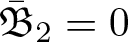 $\bar{\mathfrak{B}}_{2}=0$, we arrive at
 \begin{equation*}
\begin{aligned}
I_{4}&=\langle \mathcal{M}^{b}_{t}(\mathfrak{B}\cdot \nabla j)-\mathfrak{B}\cdot \nabla(\mathcal{M}^{b}_{t}j), \mathcal{M}^{b}_{t}\omega\rangle+\langle \mathcal{M}^{b}_{t}(\mathfrak{B}\cdot \nabla \omega)-\mathfrak{B}\cdot \nabla(\mathcal{M}^{b}_{t}\omega), \mathcal{M}^{b}_{t}j\rangle\\
&=\langle \mathcal{M}^{b}_{t}(\bar{\mathfrak{B}}_{1}\partial_{x}j)-\bar{\mathfrak{B}}_{1}\partial_{x} (\mathcal{M}^{b}_{t}j), \mathcal{M}^{b}_{t}\omega\rangle+\langle \mathcal{M}^{b}_{t}(\mathfrak{B}_{1}^{\neq}\partial_{x} j)-\mathfrak{B}_{1}^{\neq}\partial_{x} (\mathcal{M}^{b}_{t}j), \mathcal{M}^{b}_{t}\omega\rangle\\
&\ \ \ \ +\langle \mathcal{M}^{b}_{t}(\mathfrak{B}_{2}^{\neq}\partial_{y} j)-\mathfrak{B}_{2}^{\neq}\partial_{y} (\mathcal{M}^{b}_{t}j), \mathcal{M}^{b}_{t}\omega\rangle+\langle \mathcal{M}^{b}_{t}(\bar{\mathfrak{B}}_{1}\partial_{x}\omega)-\bar{\mathfrak{B}}_{1}\partial_{x} (\mathcal{M}^{b}_{t}\omega), \mathcal{M}^{b}_{t}j\rangle\\
&\ \ \ \ +\langle \mathcal{M}^{b}_{t}(\mathfrak{B}_{1}^{\neq}\partial_{x} \omega)-\mathfrak{B}_{1}^{\neq}\partial_{x} (\mathcal{M}^{b}_{t}\omega), \mathcal{M}^{b}_{t}j\rangle+\langle \mathcal{M}^{b}_{t}(\mathfrak{B}_{2}^{\neq}\partial_{y} \omega)-\mathfrak{B}_{2}^{\neq}\partial_{y} (\mathcal{M}^{b}_{t}\omega), \mathcal{M}^{b}_{t}j\rangle\\
&:=I_{41}+I_{42}+I_{43}+I_{44}+I_{45}+I_{46},
\end{aligned}
\end{equation*}
where using the fact that
 \begin{equation*}\langle \mathfrak{B}\cdot \nabla(\mathcal{M}^{b}_{t} j), \mathcal{M}^{b}_{t}\omega\rangle+\langle \mathfrak{B}\cdot \nabla(\mathcal{M}^{b}_{t}\omega), \mathcal{M}^{b}_{t} j\rangle=0.\end{equation*}
To estimate  $I_{41}$, by Plancherel’s formula, we get
 \begin{equation*}
\begin{aligned}
I_{41}
:=\sum_{k\neq0}\iint(\mathcal{M}^{b}_{t}(k,\xi)-\mathcal{M}^{b}_{t}(k,\xi-\eta))\hat{\mathfrak{B}}_{1}(0,\eta)\cdot ik&\hat{j}(k,\xi-\eta) \mathcal{M}^{b}_{t}(k,\xi)\overline{\hat{\omega}(k,\xi)}d\xi d\eta.
\end{aligned}
\end{equation*}
By the differential mean-value theorem, there holds that
 \begin{equation*}
\begin{aligned}
I_{41}
\leqslant C\sum_{k\neq 0}\iint(&\varpi^{\frac{1}{3}}|k|^{\frac{2}{3}}+\frac{|k|}{(k^{2}+\xi^{2})^{\frac{1}{2}}}+\frac{|k|}{(k^{2}+(\xi-\eta)^{2})^{\frac{1}{2}}})(\Lambda^{b}_{t}(0,\xi)+\Lambda^{b}_{t}(k,\xi-\eta))\\
& \times|\hat{j}(0,\eta)|| \hat{j}(k,\xi-\eta)||\mathcal{M}^{b}_{t}(k,\xi)\overline{\hat{\omega}(k,\xi)}|d\xi d\eta.
\end{aligned}
\end{equation*}
Hence, by Young’s convolution inequality, we obtain
 \begin{equation}
\begin{aligned}
I_{41}
&\leqslant C\|\Lambda^{b}_{t}\bar{j}\|_{L^{2}}(\|\Lambda^{b}_{t}|D_{x}|(-\Delta)^{-\frac{1}{2}}j\|_{L^{2}}\|\Lambda^{b}_{t}\omega^{\neq}\|_{L^{2}}+\|\Lambda^{b}_{t}|D_{x}|(-\Delta)^{-\frac{1}{2}}\omega\|_{L^{2}}\|\Lambda^{b}_{t}j^{\neq}\|_{L^{2}})\\
&\ \ \ \ +C\varpi^{\frac{1}{3}}\|\Lambda^{b}_{t}\bar{j}\|_{L^{2}}\|\Lambda^{b}_{t}|D_{x}|^{\frac{1}{3}}j\|_{L^{2}}\|\Lambda^{b}_{t}|D_{x}|^{\frac{1}{3}}\omega\|_{L^{2}}.
\end{aligned}
\end{equation}
Then we estimate  $I_{42}$. By Plancherel’s formula, we derive
 \begin{align*}
I_{42}
& :=\sum_{k,l}\iint(\mathcal{M}^{b}_{t}(k,\xi)-\mathcal{M}^{b}_{t}(l,\eta))\hat{\mathfrak{B}}_{1}^{\neq}(k-l,\xi-\eta)\cdot il\hat{j}(l,\eta)\\
&\cdot\mathcal{M}^{b}_{t}(k,\xi)\overline{\hat{\omega}(k,\xi)}d\xi d\eta.
\end{align*}
According to the different properties of frequency spaces  $A_{1}$ and
 $A_{2}$, one has
 \begin{equation*}
\begin{aligned}
I_{421}
\leqslant C\sum_{k,l\in A_{1}}\iint(&\Lambda^{b}_{t}(l,\eta)+\Lambda^{b}_{t}(k-l,\xi-\eta))(|k-l|+\varpi^{-\frac{1}{6}}|l|^{\frac{1}{3}}|k|^{\frac{1}{3}})\\
&\times|\hat{\mathfrak{B}}_{1}^{\neq}(k-l,\xi-\eta)||\hat{j}^{\neq}(l,\eta)||\mathcal{M}^{b}_{t}(k,\xi)\overline{\hat{\omega}(k,\xi)}|d\xi d\eta.
\end{aligned}
\end{equation*}
By Lemma 2.1, we have
 \begin{align}
I_{421}
& \leqslant C(\|\Lambda^{b}_{t}\partial_{x}\mathfrak{B}_{1}\|_{L^{2}}\|\Lambda^{b}_{t}j^{\neq}\|_{L^{2}}\|\Lambda^{b}_{t}\omega\|_{L^{2}}\nonumber\\
& \quad +\varpi^{-\frac{1}{6}}\|\Lambda^{b}_{t}\mathfrak{B}_{1}^{\neq}\|_{L^{2}}\|\Lambda^{b}_{t}|D_{x}|^{\frac{1}{3}}j\|_{L^{2}}\|\Lambda^{b}_{t}|D_{x}|^{\frac{1}{3}}\omega\|_{L^{2}}).
\end{align}
And for the second one, by Taylor’s formula and the definition of  $\mathcal{M}$, we have
 \begin{equation*}
\begin{aligned}
I_{422}
\leqslant C\sum_{k,l\in A_{2}}\iint(&\Lambda^{b}_{t}(l,\eta)+\Lambda^{b}_{t}(k-l,\xi-\eta))(\varpi^{\frac{1}{3}}|k|^{-\frac{1}{3}}|l|+1+\varpi^{\frac{1}{2}}|\eta|)\\
&\times|\hat{j}^{\neq}(k-l,\xi-\eta)||\hat{j}^{\neq}(l,\eta)||\mathcal{M}^{b}_{t}(k,\xi)\overline{\hat{\omega}(k,\xi)}|d\xi d\eta\\
\leqslant C\sum_{k,l\in A_{2}}\iint(&\Lambda^{b}_{t}(l,\eta)+\Lambda^{b}_{t}(k-l,\xi-\eta))(\varpi^{\frac{1}{3}}|k|^{\frac{1}{3}}|l|^{\frac{1}{3}}+\varpi^{\frac{2}{3}}|k|^{\frac{1}{3}}|\eta|)\\
&\times|\hat{j}^{\neq}(k-l,\xi-\eta)||\hat{j}^{\neq}(l,\eta)||\mathcal{M}^{b}_{t}(k,\xi)\overline{\hat{\omega}(k,\xi)}|d\xi d\eta.
\end{aligned}
\end{equation*}
By Lemma 2.1, it holds that
 \begin{equation}
\begin{aligned}
I_{422}\leqslant C\|\Lambda^{b}_{t}j\|_{L^{2}}(\varpi^{\frac{1}{3}}\|\Lambda^{b}_{t}|D_{x}|^{\frac{1}{3}}j\|_{L^{2}}\|\Lambda^{b}_{t}|D_{x}|^{\frac{1}{3}}\omega\|_{L^{2}}+\varpi^{\frac{2}{3}}\|\Lambda^{b}_{t}|D_{x}|^{\frac{1}{3}}j\|_{L^{2}}\|\Lambda^{b}_{t}\partial_{y}\omega\|_{L^{2}}) .
\end{aligned}
\end{equation}
Hence, combining (2.27) and (2.28) yields
 \begin{align}
I_{42}
\leqslant\,\,& C\|\Lambda^{b}_{t}(\omega,j)\|_{L^{2}}(\varpi^{-\frac{1}{6}}\|\Lambda^{b}_{t}|D_{x}|^{\frac{1}{3}}j\|_{L^{2}}\|\Lambda^{b}_{t}|D_{x}|^{\frac{1}{3}}\omega\|_{L^{2}}\nonumber\\
&\quad +\varpi^{\frac{2}{3}}\|\Lambda^{b}_{t}|D_{x}|^{\frac{1}{3}}j\|_{L^{2}}\|\Lambda^{b}_{t}\partial_{y}\omega\|_{L^{2}})\nonumber\\
&\quad +C\|\Lambda^{b}_{t}|D_{x}|(-\Delta)^{-\frac{1}{2}}j\|_{L^{2}}\|\Lambda^{b}_{t}j^{\neq}\|_{L^{2}}\|\Lambda^{b}_{t}\omega\|_{L^{2}}.
\end{align}
Similarly, to estimate  $I_{43}$. By Plancherel’s formula, we arrive at
 \begin{equation*}
\begin{aligned}
I_{43}
:=\sum_{k,l}\iint(&\mathcal{M}^{b}_{t}(k,\xi)-\mathcal{M}^{b}_{t}(k-l,\xi-\eta))\hat{\mathfrak{B}}_{2}^{\neq}(l,\eta)\cdot i(\xi-\eta)\hat{j}(k-l,\xi-\eta)\\
&\times\mathcal{M}^{b}_{t}(k,\xi)\overline{\hat{\omega}(k,\xi)}d\xi d\eta.
\end{aligned}
\end{equation*}
By Lemma 2.1 and the boundedness of multiplier  $\mathcal{M}$, we deduce
 \begin{equation}
\begin{aligned}
I_{43}
&\leqslant C\|\Lambda^{b}_{t}|D_{x}|(-\Delta)^{-\frac{1}{2}}j\|_{L^{2}}\|\Lambda^{b}_{t}\partial_{y}j\|_{L^{2}}\|\Lambda^{b}_{t}\omega\|_{L^{2}}.
\end{aligned}
\end{equation}
Next, the estimate of  $I_{44}$ is given. By Plancherel’s formula, we get
 \begin{align*}
I_{44}
&:=\sum_{k\neq0}\iint(\mathcal{M}^{b}_{t}(k,\xi)-\mathcal{M}^{b}_{t}(k,\xi-\eta))\hat{\mathfrak{B}}_{1}(0,\eta)\\
&\quad\cdot ik\hat{\omega}(k,\xi-\eta)\cdot\mathcal{M}^{b}_{t}(k,\xi)\overline{\hat{j}(k,\xi)}d\xi d\eta.
\end{align*}
By the differential mean-value theorem, there holds that
 \begin{equation*}
\begin{aligned}
I_{44}
\leqslant C\sum_{k\neq 0}\iint(&\varpi^{\frac{1}{3}}|k|^{\frac{2}{3}}+\frac{|k|}{(k^{2}+\xi^{2})^{\frac{1}{2}}}+\frac{|k|}{(k^{2}+(\xi-\eta)^{2})^{\frac{1}{2}}})(\Lambda^{b}_{t}(0,\xi)+\Lambda^{b}_{t}(k,\xi-\eta))\\
&\times|\hat{j}(0,\eta)|| \hat{\omega}(k,\xi-\eta)||\mathcal{M}^{b}_{t}(k,\xi)\overline{\hat{j}(k,\xi)}|d\xi d\eta.
\end{aligned}
\end{equation*}
Hence, by Young’s convolution inequality, we obtain
 \begin{equation}
\begin{aligned}
I_{44}
&\leqslant C\|\Lambda^{b}_{t}\bar{j}\|_{L^{2}}(\|\Lambda^{b}_{t}|D_{x}|(-\Delta)^{-\frac{1}{2}}j\|_{L^{2}}\|\Lambda^{b}_{t}\omega^{\neq}\|_{L^{2}}+\|\Lambda^{b}_{t}|D_{x}|(-\Delta)^{-\frac{1}{2}}\omega\|_{L^{2}}\|\Lambda^{b}_{t}j^{\neq}\|_{L^{2}})\\
&\ \ \ \ +C\varpi^{\frac{1}{3}}\|\Lambda^{b}_{t}\bar{j}\|_{L^{2}}\|\Lambda^{b}_{t}|D_{x}|^{\frac{1}{3}}j\|_{L^{2}}\|\Lambda^{b}_{t}|D_{x}|^{\frac{1}{3}}\omega\|_{L^{2}}.
\end{aligned}
\end{equation}
Then we estimate  $I_{45}$. By Plancherel’s formula, we derive
 \begin{equation*}
\begin{aligned}
I_{45}
:=\sum_{k,l}\iint(\mathcal{M}^{b}_{t}(k,\xi)-\mathcal{M}^{b}_{t}(l,\eta))\hat{\mathfrak{B}}_{1}^{\neq}(k-l,\xi-\eta)\cdot il\hat{\omega}(l,\eta)\mathcal{M}^{b}_{t}(k,\xi)\overline{\hat{j}(k,\xi)}d\xi d\eta.
\end{aligned}
\end{equation*}
According to the different properties of frequency spaces  $A_{1}$ and
 $A_{2}$, one has
 \begin{equation*}
\begin{aligned}
I_{451}
\leqslant C\sum_{k,l\in A_{1}}\iint(&\Lambda^{b}_{t}(l,\eta)+\Lambda^{b}_{t}(k-l,\xi-\eta))(|k-l|+\varpi^{-\frac{1}{6}}|l|^{\frac{1}{3}}|k|^{\frac{1}{3}})\\
&\times|\hat{\mathfrak{B}}_{1}^{\neq}(k-l,\xi-\eta)||\hat{\omega}^{\neq}(l,\eta)||\mathcal{M}^{b}_{t}(k,\xi)\overline{\hat{j}(k,\xi)}|d\xi d\eta.
\end{aligned}
\end{equation*}
By Lemma 2.1, we get
 \begin{align}
I_{451}
& \leqslant C(\|\Lambda^{b}_{t}\partial_{x}\mathfrak{B}_{1}\|_{L^{2}}\|\Lambda^{b}_{t}\omega^{\neq}\|_{L^{2}}\|\Lambda^{b}_{t}j\|_{L^{2}}\nonumber\\
&\quad +\varpi^{-\frac{1}{6}}\|\Lambda^{b}_{t}\mathfrak{B}_{1}^{\neq}\|_{L^{2}}\|\Lambda^{b}_{t}|D_{x}|^{\frac{1}{3}}j\|_{L^{2}}\|\Lambda^{b}_{t}|D_{x}|^{\frac{1}{3}}\omega\|_{L^{2}}).
\end{align}
And for the second one, by Taylor’s formula and the definition of  $\mathcal{M}$, we have
 \begin{equation*}
\begin{aligned}
I_{452}
\leqslant C\sum_{k,l\in A_{2}}\iint(&\Lambda^{b}_{t}(l,\eta)+\Lambda^{b}_{t}(k-l,\xi-\eta))(\varpi^{\frac{1}{3}}|k|^{-\frac{1}{3}}|l|+1+\varpi^{\frac{1}{2}}|\eta|)\\
&\ \ \ \ \times|\hat{j}^{\neq}(k-l,\xi-\eta)||\hat{\omega}^{\neq}(l,\eta)||\mathcal{M}^{b}_{t}(k,\xi)\overline{\hat{j}(k,\xi)}|d\xi d\eta\\
\leqslant C\sum_{k,l\in A_{2}}\iint(&\Lambda^{b}_{t}(l,\eta)+\Lambda^{b}_{t}(k-l,\xi-\eta))(\varpi^{\frac{1}{3}}|k|^{\frac{1}{3}}|l|^{\frac{1}{3}}+\varpi^{\frac{2}{3}}|k|^{\frac{1}{3}}|\eta|)\\
&\ \ \ \ \times|\hat{j}^{\neq}(k-l,\xi-\eta)||\hat{\omega}^{\neq}(l,\eta)||\mathcal{M}^{b}_{t}(k,\xi)\overline{\hat{j}(k,\xi)}|d\xi d\eta.
\end{aligned}
\end{equation*}
By Lemma 2.1, it holds that
 \begin{equation}
\begin{aligned}
I_{452}\leqslant C\|\Lambda^{b}_{t}j\|_{L^{2}}\|\Lambda^{b}_{t}|D_{x}|^{\frac{1}{3}}j\|_{L^{2}}(\varpi^{\frac{1}{3}}\|\Lambda^{b}_{t}|D_{x}|^{\frac{1}{3}}\omega\|_{L^{2}}+\varpi^{\frac{2}{3}}\|\Lambda^{b}_{t}\partial_{y}\omega\|_{L^{2}}) .
\end{aligned}
\end{equation}
Hence, combining (2.32) and (2.33) yields
 \begin{equation}
\begin{aligned}
I_{45}
\leqslant&
\,\,C\|\Lambda^{b}_{t}(\omega,j)\|_{L^{2}}\|\Lambda^{b}_{t}|D_{x}|^{\frac{1}{3}}j\|_{L^{2}}(\varpi^{-\frac{1}{6}}\|\Lambda^{b}_{t}|D_{x}|^{\frac{1}{3}}\omega\|_{L^{2}}+\varpi^{\frac{2}{3}}\|\Lambda^{b}_{t}\partial_{y}\omega\|_{L^{2}})\\
&\ \ \ \ \ \ +C\|\Lambda^{b}_{t}|D_{x}|(-\Delta)^{-\frac{1}{2}}j\|_{L^{2}}\|\Lambda^{b}_{t}j\|_{L^{2}}\|\Lambda^{b}_{t}\omega^{\neq}\|_{L^{2}}.
\end{aligned}
\end{equation}
Next estimate  $I_{46}$. By Plancherel’s formula, we arrive at
 \begin{equation*}
\begin{aligned}
I_{46}
:=\sum_{k,l}\iint(&\mathcal{M}^{b}_{t}(k,\xi)-\mathcal{M}^{b}_{t}(k-l,\xi-\eta))\hat{\mathfrak{B}}_{2}^{\neq}(l,\eta)\cdot i(\xi-\eta)\hat{\omega}(k-l,\xi-\eta)\\
&\times\mathcal{M}^{b}_{t}(k,\xi)\overline{\hat{j}(k,\xi)}d\xi d\eta.
\end{aligned}
\end{equation*}
By Lemma 2.1 and the boundedness of multiplier  $\mathcal{M}$, we deduce
 \begin{equation}
\begin{aligned}
I_{46}
&\leqslant C\|\Lambda^{b}_{t}|D_{x}|(-\Delta)^{-\frac{1}{2}}j\|_{L^{2}}\|\Lambda^{b}_{t}j\|_{L^{2}}\|\Lambda^{b}_{t}\partial_{y}\omega\|_{L^{2}}.
\end{aligned}
\end{equation}
By combining (2.26), (2.29), (2.30), (2.31), (2.34), and (2.35), we have
 \begin{equation}
\begin{aligned}
I_{4}
&\leqslant C\|\Lambda^{b}_{t}(\omega,j)\|_{L^{2}}\|\Lambda^{b}_{t}|D_{x}|^{\frac{1}{3}}j\|_{L^{2}}(\varpi^{-\frac{1}{6}}\|\Lambda^{b}_{t}|D_{x}|^{\frac{1}{3}}\omega\|_{L^{2}}+\varpi^{\frac{2}{3}}\|\Lambda^{b}_{t}\partial_{y}\omega\|_{L^{2}})\\
&\ \ \ \ +C\|\Lambda^{b}_{t}(\omega,j)\|_{L^{2}}(\|\Lambda^{b}_{t}|D_{x}|(-\Delta)^{-\frac{1}{2}}(\omega,j)\|_{L^{2}}\|\Lambda^{b}_{t}(\omega,j)^{\neq}\|_{L^{2}}+\|\Lambda^{b}_{t}\partial_{y}j\|_{L^{2}}).
\end{aligned}
\end{equation}
Thus, combining (2.11), (2.12), (2.18), (2.25), (2.36), and (2.19), it can be concluded that
 \begin{align}
&\frac{d}{dt}\|\mathcal{M}^{b}_{t}(\omega,j)\|_{L^{2}}^{2}+\varpi\|\mathcal{M}^{b}_{t}\partial_{y}(\omega,j)\|_{L^{2}}^{2}+\frac{1}{4}\varpi^{\frac{1}{3}}\|\mathcal{M}^{b}_{t}\vert D_{x}\vert^{\frac{1}{3}}(\omega,j)\|_{L^{2}}^{2}\nonumber\\
&\quad +\|\mathcal{M}^{b}_{t}|D_{x}|(-\Delta)^{-\frac{1}{2}}(\omega,j)\|_{L^{2}}^{2}\nonumber\\
& \qquad \leqslant C\|\Lambda^{b}_{t}(\omega,j)\|_{L^{2}}(\varpi^{-\frac{1}{6}}\|\Lambda^{b}_{t}|D_{x}|^{\frac{1}{3}}(\omega,j)\|_{L^{2}}^{2}+\varpi^{\frac{2}{3}}\|\Lambda^{b}_{t}|D_{x}|^{\frac{1}{3}}(\omega,j)\|_{L^{2}}\nonumber\\
&\quad\|\Lambda^{b}_{t}\partial_{y}(\omega,j)\|_{L^{2}})+C\|\Lambda^{b}_{t}(\omega,j)\|_{L^{2}}\|\Lambda^{b}_{t}|D_{x}|(-\Delta)^{-\frac{1}{2}}(\omega,j)\|_{L^{2}}(\|\Lambda^{b}_{t}\partial_{y}(\omega,j)\|_{L^{2}}\nonumber\\
&\quad +\|\Lambda^{b}_{t}|D_{x}|^{\frac{1}{3}}(\omega,j)^{\neq}\|_{L^{2}})\nonumber\\
& -\langle 4\partial_{xy}\Lambda^{b}_{t}\phi, \mathcal{M} \Lambda^{b}_{t}j\rangle.
\end{align}
To complete this estimate, it is necessary to deal with the linear term,  $-\langle 4\partial_{xy}\Lambda^{b}_{t}\phi, \mathcal{M} \Lambda^{b}_{t}j\rangle$. To be precise,
 \begin{equation}
\begin{aligned}
-\langle 4\partial_{xy}\Lambda^{b}_{t}\phi, \mathcal{M} \Lambda^{b}_{t}j\rangle=\langle 4\partial_{x}\Lambda^{b}_{t}\phi, \mathcal{M} \Lambda^{b}_{t}\partial_{y}j\rangle \leqslant C\mu^{-1}\|\Lambda^{b}_{t}\partial_{x}\phi\|_{L^{2}}^{2}+ \frac{\mu}{8}\|\Lambda^{b}_{t}\partial_{y}j\|_{L^{2}}^{2}.
\end{aligned}
\end{equation}
Integrating (2.37) in time and then from (2.2) and (2.3), it deduces that
 \begin{equation}
\begin{aligned}
&E_{1}^{2}(t)\leqslant E_{1}^{2}(0)+C\varpi^{-\frac{1}{2}}E_{1}^{3}(t)+C\mu^{-\frac{4}{3}}E_{2}^{2}(t)
\end{aligned}
\end{equation}
for a positive constant  $C$ and any
 $t \gt 0$. Hence, the proof of Proposition 2.1 is completed.
2.4. Proof of Proposition 2.2
In this section, we devote to the proof of Proposition 2.2. According to (2.38), the estimate of  $\|\Lambda^{b}_{t}|D_{x}|\phi\|_{L^{2}L^{2}}$ is necessary for obtaining the expected stability result. Next, we give the estimate of the fractional horizontal derivative of
 $\phi$.
Proof of Proposition 2.2
First, by applying the operator  $\Lambda^{b}_{t}$ to
 $(1.3)_{2}$ and Lemma 2.1, taking the
 $L^{2}$ inner product of the equation with
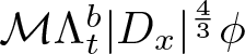 $\mathcal{M}\Lambda^{b}_{t}|D_{x}|^{\frac{4}{3}}\phi$ yields
 \begin{equation}
\begin{aligned}
\langle \partial_{t}\Lambda^{b}_{t}\phi+y\partial_{x}\Lambda^{b}_{t}\phi-\mu\partial_{yy} \Lambda^{b}_{t}\phi, \mathcal{M} \Lambda^{b}_{t}|D_{x}|^{\frac{4}{3}}\phi\rangle =\langle \Lambda^{b}_{t}(-u\cdot \nabla \phi), \mathcal{M} \Lambda^{b}_{t}|D_{x}|^{\frac{4}{3}}\phi\rangle:=-G.
\end{aligned}
\end{equation}
Then according to the properties of multiplier  $\mathcal{M} $ and (1.7), we have
 \begin{equation}
\begin{aligned}
LHS~~ of~~ (2.40)\geqslant & \frac{1}{2}\frac{d}{dt}\|\mathcal{M}^{b}_{t}|D_{x}|^{\frac{2}{3}}\phi\|_{L^{2}}^{2} +\frac{1}{2}\|\mathcal{M}^{b}_{t}|D_{x}|^{\frac{5}{3}}(-\Delta)^{-\frac{1}{2}}\phi\|_{L^{2}}^{2}\\
&+\frac{1}{2}\mu\|\mathcal{M}^{b}_{t}\partial_{y}|D_{x}|^{\frac{2}{3}}\phi\|_{L^{2}}^{2}+\frac{1}{8}\varpi^{\frac{1}{3}}\|\mathcal{M}^{b}_{t}|D_{x}|\phi\|_{L^{2}}^{2}.
\end{aligned}
\end{equation}
Next, the estimate of the nonlinear term is given. By  ${\rm div}\,u=0$ and
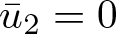 $\bar{u}_{2}=0$, we arrive at
 \begin{equation*}
\begin{aligned}
G&=\langle \mathcal{M}^{b}_{t}\vert D_{x}\vert^{\frac{2}{3}}(u\cdot \nabla \phi)-u\cdot \nabla(\mathcal{M}^{b}_{t} \vert D_{x}\vert^{\frac{2}{3}}\phi), \mathcal{M}^{b}_{t}\vert D_{x}\vert^{\frac{2}{3}}\phi\rangle\\
&=\langle \mathcal{M}^{b}_{t}(\bar{u}_{1}\partial_{x}\vert D_{x}\vert^{\frac{2}{3}} \phi)-\bar{u}_{1}\partial_{x} (\mathcal{M}^{b}_{t}\vert D_{x}\vert^{\frac{2}{3}} \phi), \mathcal{M}^{b}_{t}\vert D_{x}\vert^{\frac{2}{3}}\phi\rangle\\
&\ \ \ \ +\langle \mathcal{M}^{b}_{t}(u_{1}^{\neq}\partial_{x} \vert D_{x}\vert^{\frac{2}{3}}\phi)-u_{1}^{\neq}\partial_{x} (\mathcal{M}^{b}_{t} \vert D_{x}\vert^{\frac{2}{3}}\phi), \mathcal{M}^{b}_{t}\vert D_{x}\vert^{\frac{2}{3}}\phi\rangle\\
&\ \ \ \ +\langle \mathcal{M}^{b}_{t}(u_{2}^{\neq}\partial_{y} \vert D_{x}\vert^{\frac{2}{3}}\phi)-u_{2}^{\neq}\partial_{y} (\mathcal{M}^{b}_{t} \vert D_{x}\vert^{\frac{2}{3}}\phi), \mathcal{M}^{b}_{t}\vert D_{x}\vert^{\frac{2}{3}}\phi\rangle\\
&\ \ \ \ +\langle \mathcal{M}^{b}_{t}(\vert D_{x}\vert^{\frac{2}{3}}(u\cdot \nabla \phi)-(u\cdot \nabla \vert D_{x}\vert^{\frac{2}{3}}\phi)), \mathcal{M}^{b}_{t}\vert D_{x}\vert^{\frac{2}{3}}\phi\rangle\\
&:=G_{1}+G_{2}+G_{3}+G_{4}.
\end{aligned}
\end{equation*}
To estimate  $G_{1}$, by Plancherel’s formula, we get
 \begin{equation*}
\begin{aligned}
G_{1}
\leqslant\sum_{k\neq0}\iint&|\mathcal{M}^{b}_{t}(k,\xi)-\mathcal{M}^{b}_{t}(k,\xi-\eta)||\hat{u}_{1}(0,\eta)|\cdot |k|^{\frac{5}{3}}|\hat{\phi}(k,\xi-\eta)|\\
&\times\mathcal{M}^{b}_{t}(k,\xi)|k|^{\frac{2}{3}}|\overline{\hat{\phi}(k,\xi)}|d\xi d\eta.
\end{aligned}
\end{equation*}
By the differential mean-value theorem, there holds
 \begin{equation*}
\begin{aligned}
G_{1}
\leqslant C\sum_{k\neq 0}\iint(&\varpi^{\frac{1}{3}}|k|^{\frac{2}{3}}+\frac{|k|}{(k^{2}+\xi^{2})^{\frac{1}{2}}}+\frac{|k|}{(k^{2}+(\xi-\eta)^{2})^{\frac{1}{2}}})(\Lambda^{b}_{t}(0,\xi)+\Lambda^{b}_{t}(k,\xi-\eta))\\
&\times|\hat{\omega}(0,\eta)|| \hat{\phi}(k,\xi-\eta)||\mathcal{M}^{b}_{t}(k,\xi)|k|^{\frac{4}{3}}\overline{\hat{\phi}(k,\xi)}|d\xi d\eta.
\end{aligned}
\end{equation*}
Hence, by Young’s convolution inequality, we obtain
 \begin{equation}
\begin{aligned}
G_{1}
\leqslant C(\varpi^{\frac{1}{3}}\|\Lambda^{b}_{t}\bar{\omega}\|_{L^{2}}\|\Lambda^{b}_{t}|D_{x}|\phi\|_{L^{2}}^{2}+\|\Lambda^{b}_{t}\bar{\omega}\|_{L^{2}}\|\Lambda^{b}_{t}|D_{x}|^{\frac{5}{3}}(-\Delta)^{-\frac{1}{2}}\phi\|_{L^{2}}\|\Lambda^{b}_{t}|D_{x}|^{\frac{2}{3}}\phi\|_{L^{2}}).
\end{aligned}
\end{equation}
Then we estimate  $G_{2}$. By Plancherel’s formula, we derive
 \begin{equation*}
\begin{aligned}
G_{2}
\leqslant\sum_{k,l}\iint&|\mathcal{M}^{b}_{t}(k,\xi)-\mathcal{M}^{b}_{t}(l,\eta)||\hat{u}_{1}^{\neq}(k-l,\xi-\eta)|\cdot |l|^{\frac{2}{3}}|\hat{\phi}(l,\eta)|\\
&\times\mathcal{M}^{b}_{t}(k,\xi)|k|^{\frac{2}{3}}|\overline{\hat{\phi}(k,\xi)}|d\xi d\eta.
\end{aligned}
\end{equation*}
According to the different properties of frequency spaces  $A_{1}$ and
 $A_{2}$, one has
 \begin{equation*}
\begin{aligned}
G_{21}
\leqslant C\sum_{k,l\in A_{1}}\iint(&\Lambda^{b}_{t}(l,\eta)+\Lambda^{b}_{t}(k-l,\xi-\eta))(|k-l|+\varpi^{-\frac{1}{6}}|l|^{\frac{1}{3}}|k|^{\frac{1}{3}})|l|^{\frac{2}{3}}\\
&\times|\hat{u}_{1}^{\neq}(k-l,\xi-\eta)||\hat{\phi}^{\neq}(l,\eta)|\mathcal{M}^{b}_{t}(k,\xi)|k|^{\frac{2}{3}}|\overline{\hat{\phi}(k,\xi)}|d\xi d\eta.
\end{aligned}
\end{equation*}
By Lemma 2.1, we have
 \begin{equation}
\begin{aligned}
G_{21}
&\leqslant C(\|\Lambda^{b}_{t}\partial_{x}u_{1}\|_{L^{2}}\|\Lambda^{b}_{t}\vert D_{x}\vert^{\frac{2}{3}}\phi^{\neq}\|_{L^{2}}\|\Lambda^{b}_{t}\vert D_{x}\vert^{\frac{2}{3}}\phi\|_{L^{2}}+\varpi^{-\frac{1}{6}}\|\Lambda^{b}_{t}u_{1}^{\neq}\|_{L^{2}}\|\Lambda^{b}_{t}|D_{x}|\phi\|_{L^{2}}^{2}).
\end{aligned}
\end{equation}
And for the second one, by Taylor’s formula and the definition of  $\mathcal{M}$, one has
 \begin{equation*}
\begin{aligned}
G_{22}
\leqslant C\sum_{k,l\in A_{2}}\iint(&\Lambda^{b}_{t}(l,\eta)+\Lambda^{b}_{t}(k-l,\xi-\eta))(\varpi^{\frac{1}{3}}|k|^{-\frac{1}{3}}|l|+1+\varpi^{\frac{1}{2}}|\eta|)|l|^{\frac{2}{3}}\\
&\times|\hat{\omega}^{\neq}(k-l,\xi-\eta)||\hat{\phi}^{\neq}(l,\eta)|\mathcal{M}^{b}_{t}(k,\xi)|k|^{\frac{2}{3}}|\overline{\hat{\phi}(k,\xi)}|d\xi d\eta\\
\leqslant C\sum_{k,l\in A_{2}}\iint(&\Lambda^{b}_{t}(l,\eta)+\Lambda^{b}_{t}(k-l,\xi-\eta))(\varpi^{\frac{1}{3}}|k|^{\frac{1}{3}}|l|^{\frac{1}{3}}+\varpi^{\frac{2}{3}}|k|^{\frac{1}{3}}|\eta|)|l|^{\frac{2}{3}}\\
&\times|\hat{\omega}^{\neq}(k-l,\xi-\eta)||\hat{\phi}^{\neq}(l,\eta)|\mathcal{M}^{b}_{t}(k,\xi)|k|^{\frac{2}{3}}|\overline{\hat{\phi}(k,\xi)}|d\xi d\eta.
\end{aligned}
\end{equation*}
By Lemma 2.1, it holds that
 \begin{equation}
\begin{aligned}
G_{22}\leqslant C(\varpi^{\frac{1}{3}}\|\Lambda^{b}_{t}\omega\|_{L^{2}}\|\Lambda^{b}_{t}|D_{x}|\phi\|_{L^{2}}^{2}+\varpi^{\frac{2}{3}}\|\Lambda^{b}_{t}\omega\|_{L^{2}}\|\Lambda^{b}_{t}|D_{x}|\phi\|_{L^{2}}\|\Lambda^{b}_{t}\partial_{y}|D_{x}|^{\frac{2}{3}}\phi\|_{L^{2}}) .
\end{aligned}
\end{equation}
Hence, combining (2.43) and (2.44) yields
 \begin{equation}
\begin{aligned}
G_{2}
\leqslant& \,\,C\|\Lambda^{b}_{t}\omega\|_{L^{2}}(\varpi^{-\frac{1}{6}}\|\Lambda^{b}_{t}|D_{x}|\phi\|_{L^{2}}^{2}+\varpi^{\frac{2}{3}}\|\Lambda^{b}_{t}|D_{x}|\phi\|_{L^{2}}\|\Lambda^{b}_{t}\partial_{y}|D_{x}|^{\frac{2}{3}}\phi\|_{L^{2}})\\
&\ \ \ \ \ \ +C\|\Lambda^{b}_{t}\partial_{x}u_{1}\|_{L^{2}}\|\Lambda^{b}_{t}|D_{x}|^{\frac{2}{3}}\phi^{\neq}\|_{L^{2}}\|\Lambda^{b}_{t}|D_{x}|^{\frac{2}{3}}\phi\|_{L^{2}}.
\end{aligned}
\end{equation}
Next, estimate  $G_{3}$. By Plancherel’s formula, we arrive at
 \begin{equation*}
\begin{aligned}
G_{3}
\leqslant\sum_{k,l}\iint&|\mathcal{M}^{b}_{t}(k,\xi)-\mathcal{M}^{b}_{t}(k-l,\xi-\eta)||\hat{u}_{2}^{\neq}(l,\eta)|\cdot |k-l|^{\frac{2}{3}}|\xi-\eta|\\
&\times|\hat{\phi}(k-l,\xi-\eta)|\mathcal{M}^{b}_{t}(k,\xi)|k|^{\frac{2}{3}}|\overline{\hat{\phi}(k,\xi)}|d\xi d\eta.
\end{aligned}
\end{equation*}
By Lemma 2.1 and the boundedness of multiplier  $\mathcal{M}$, we deduce
 \begin{align}
G_{3}
&\leqslant C\|\Lambda^{b}_{t}u_{2}\|_{L^{2}}\|\Lambda^{b}_{t}\partial_{y}\vert D_{x}\vert^{\frac{2}{3}}\phi\|_{L^{2}}\|\Lambda^{b}_{t}\vert D_{x}\vert^{\frac{2}{3}}\phi\|_{L^{2}}.
\end{align}
Then the estimate of  $G_{4}$ is given. It holds that
 \begin{align}
G_{4}=&\langle \mathcal{M}^{b}_{t}(\vert D_{x}\vert^{\frac{2}{3}}(u\cdot \nabla \bar{\phi})+\vert D_{x}\vert^{\frac{2}{3}}(u\cdot \nabla \phi^{\neq})-(u\cdot \nabla \vert D_{x}\vert^{\frac{2}{3}}\phi^{\neq})), \mathcal{M}^{b}_{t}\vert D_{x}\vert^{\frac{2}{3}}\phi\rangle\nonumber\\
&=\langle \mathcal{M}^{b}_{t}(\vert D_{x}\vert^{\frac{2}{3}}u_2\partial_{y}\bar{\phi}), \mathcal{M}^{b}_{t}\vert D_{x}\vert^{\frac{2}{3}}\phi\rangle+\langle \mathcal{M}^{b}_{t}[ \vert D_{x}\vert^{\frac{2}{3}},u\cdot \nabla]\phi^{\neq}, \mathcal{M}^{b}_{t}\vert D_{x}\vert^{\frac{2}{3}}\phi\rangle\nonumber\\
\quad \leqslant
& C\|\Lambda^{b}_{t}\vert D_{x}\vert^{\frac{2}{3}}\phi\|_{L^{2}}(\|\Lambda^{b}_{t}\vert D_{x}\vert^{\frac{2}{3}}u_{2}\|_{L^{2}}\|\Lambda^{b}_{t}\partial_{y}\bar{\phi}\|_{L^{2}}+\|\Lambda^{b}_{t}\vert D_{x}\vert^{\frac{2}{3}}\phi\|_{L^{2}}\|\Lambda^{b}_{t}\omega\|_{L^{2}})\nonumber\\
&\quad +C\|\Lambda^{b}_{t}\vert D_{x}\vert^{\frac{2}{3}}\phi\|_{L^{2}}(\|\Lambda^{b}_{t}\vert D_{x}\vert^{\frac{2}{3}}u_{2}\|_{L^{2}}\|\Lambda^{b}_{t}\partial_{y}\phi^{\neq}\|_{L^{2}}\nonumber\\
&\quad +\|\Lambda^{b}_{t}\vert D_{x}\vert^{\frac{2}{3}}u_{1}\|_{L^{2}}\|\Lambda^{b}_{t}\vert D_{x}\vert\phi\|_{L^{2}}).
\end{align}
Combining (2.42), (2.45), (2.46), and (2.47), we have
 \begin{align}
G
&\leqslant C\|\Lambda^{b}_{t}\omega\|_{L^{2}}(\varpi^{\frac{2}{3}}\|\Lambda^{b}_{t}|D_{x}|\phi\|_{L^{2}}\|\Lambda^{b}_{t}\partial_{y}\vert D_{x}\vert^{\frac{2}{3}}\phi\|_{L^{2}}\nonumber\\
&\quad +\|\Lambda^{b}_{t}|D_{x}|^{\frac{5}{3}}(-\Delta)^{-\frac{1}{2}}\phi\|_{L^{2}}\|\Lambda^{b}_{t}\vert D_{x}\vert^{\frac{2}{3}}\phi\|_{L^{2}})\nonumber\\
&\quad +C\|\Lambda^{b}_{t}|D_{x}|^{\frac{2}{3}}\phi\|_{L^{2}}\|\Lambda^{b}_{t}|D_{x}|(-\Delta)^{-\frac{1}{2}}\omega^{\neq}\|_{L^{2}}(\|\Lambda^{b}_{t}|D_{x}|\phi\|_{L^{2}}\nonumber\\
&\quad + \|\Lambda^{b}_{t}\partial_{y}|D_{x}|^{\frac{2}{3}}\phi\|_{L^{2}})\nonumber\\
&\quad + C\varpi^{-\frac{1}{6}}\|\Lambda^{b}_{t}\omega\|_{L^{2}}\|\Lambda^{b}_{t}|D_{x}|\phi\|_{L^{2}}^{2}\nonumber\\
&\quad +C\|\Lambda^{b}_{t}\vert D_{x}\vert^{\frac{2}{3}}\phi\|_{L^{2}}\|\Lambda^{b}_{t}\vert D_{x}\vert^{\frac{2}{3}}u_{2}\|_{L^{2}}\|\Lambda^{b}_{t}\partial_{y}\bar{\phi}\|_{L^{2}}.
\end{align}
From (2.41) and (2.48), we deduce
 \begin{align}
&\frac{d}{dt}\|\mathcal{M}^{b}_{t}|D_{x}|^{\frac{2}{3}}\phi\|_{L^{2}}^{2}+\mu\|\mathcal{M}^{b}_{t}\partial_{y}|D_{x}|^{\frac{2}{3}}\phi\|_{L^{2}}^{2}+\frac{1}{4}\varpi^{\frac{1}{3}}\|\mathcal{M}^{b}_{t}|D_{x}|\phi\|_{L^{2}}^{2}\nonumber\\
&\quad+\|\mathcal{M}^{b}_{t}|D_{x}|^{\frac{5}{3}}(-\Delta)^{-\frac{1}{2}}\phi\|_{L^{2}}^{2}\nonumber\\
&\qquad \leqslant C\|\Lambda^{b}_{t}\omega\|_{L^{2}}\|\Lambda^{b}_{t}|D_{x}|\phi\|_{L^{2}}(\varpi^{\frac{2}{3}}\|\Lambda^{b}_{t}\partial_{y}\vert D_{x}\vert^{\frac{2}{3}}\phi\|_{L^{2}}\nonumber\\
&\quad+\|\Lambda^{b}_{t}|D_{x}|^{\frac{5}{3}}(-\Delta)^{-\frac{1}{2}}\phi\|_{L^{2}})\nonumber\\
&\quad +C\|\Lambda^{b}_{t}|D_{x}|^{\frac{2}{3}}\phi\|_{L^{2}}\|\Lambda^{b}_{t}|D_{x}|(-\Delta)^{-\frac{1}{2}}\omega\|_{L^{2}}(\|\Lambda^{b}_{t}|D_{x}|\phi\|_{L^{2}}\nonumber\\
&\quad+ \|\Lambda^{b}_{t}\partial_{y}|D_{x}|^{\frac{2}{3}}\phi\|_{L^{2}})\nonumber\\
&\quad + C\varpi^{-\frac{1}{6}}\|\Lambda^{b}_{t}\omega\|_{L^{2}}\|\Lambda^{b}_{t}|D_{x}|\phi\|_{L^{2}}^{2}\nonumber\\
&\quad +C\|\Lambda^{b}_{t}\vert D_{x}\vert^{\frac{2}{3}}\phi\|_{L^{2}}\|\Lambda^{b}_{t}|D_{x}|(-\Delta)^{-\frac{1}{2}}\omega\|_{L^{2}}\|\Lambda^{b}_{t}\partial_{y}\bar{\phi}\|_{L^{2}}.
\end{align}
Integrating (2.49) in time, one has that
 \begin{equation*}
\begin{aligned}
&E_{2}^{2}(t)\leqslant E_{2}^{2}(0)+C\varpi^{-\frac{1}{2}}E_{1}(t)E_{2}^{2}(t)+C\varpi^{-\frac{1}{6}}E_{1}(t)E_{2}(t)E_{3}(t)
\end{aligned}
\end{equation*}
for some positive constant  $C$ and any
 $t \gt 0$. Hence, the proof of Proposition 2.2 is completed.
2.5. Proof of Proposition 2.3
In this section, we devote to the proof of Proposition 2.3. It should be noted that, in order to obtain the expected result, we need to precisely estimate 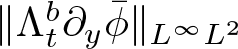 $\|\Lambda^{b}_{t}\partial_{y}\bar{\phi}\|_{L^{\infty}L^{2}}$. This means that an additional functional is required, i.e.,
 $E_{3}(t)$. Next, we give the estimate of the vertical derivative of
 $\bar{\phi}$.
Proof of Proposition 2.3
Firstly, the equation of  $\Lambda^{b}_{t}\bar{\phi}$ is as follows:
 \begin{equation}
\begin{aligned}
\partial_{t}\Lambda^{b}_{t}\bar{\phi}-\mu\partial_{yy}\Lambda^{b}_{t}\bar{\phi}=-\Lambda^{b}_{t}(\overline{u\cdot \nabla \phi})=-\Lambda^{b}_{t}(\overline{u_{1}^{\neq}\partial_{x}\phi})-\Lambda^{b}_{t}(\overline{u_{2}\partial_{y}\phi^{\neq}}).
\end{aligned}
\end{equation}
Taking the  $L^{2}$ inner product of the equation with
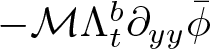 $-\mathcal{M}\Lambda^{b}_{t}\partial_{yy}\bar{\phi}$ yields
 \begin{equation}
\begin{aligned}
\langle \partial_{t}\Lambda^{b}_{t}\bar{\phi}-\mu\partial_{yy} \Lambda^{b}_{t}\bar{\phi}, -\mathcal{M} \Lambda^{b}_{t}\partial_{yy}\bar{\phi}\rangle =\langle \Lambda^{b}_{t}(\overline{u_{1}^{\neq}\partial_{x}\phi})+\Lambda^{b}_{t}(\overline{u_{2}\partial_{y}\phi^{\neq}}), \mathcal{M} \Lambda^{b}_{t}\partial_{yy}\bar{\phi}\rangle.
\end{aligned}
\end{equation}
Then by the boundedness of multiplier  $\mathcal{M}$, we get that
 \begin{equation}
\begin{aligned}
&\frac{d}{dt}\|\mathcal{M}^{b}_{t}\partial_{y}\bar{\phi}\|_{L^{2}}^{2}+2\mu\|\mathcal{M}^{b}_{t}\partial_{yy}\bar{\phi}\|_{L^{2}}^{2}\\
&= -2\langle \Lambda^{b}_{t}\partial_{y}(\overline{u_{1}^{\neq}\partial_{x}\phi})+\Lambda^{b}_{t}\partial_{y}(\overline{u_{2}\partial_{y}\phi^{\neq}}), \mathcal{M} \Lambda^{b}_{t}\partial_{y}\bar{\phi}\rangle\\
&\leqslant C\|\Lambda^{b}_{t}\partial_{y}\bar{\phi}\|_{L^{2}}(\|\Lambda^{b}_{t}\nabla u_{1}^{\neq}\|_{L^{2}}\|\Lambda^{b}_{t}\nabla\phi^{\neq}\|_{L^{2}}+\|\Lambda^{b}_{t}u^{\neq}\|_{L^{2}}\|\Lambda^{b}_{t}j^{\neq}\|_{L^{2}})\\
&\leqslant C\|\Lambda^{b}_{t}\partial_{y}\bar{\phi}\|_{L^{2}}\|\Lambda^{b}_{t}|D_{x}|(-\Delta)^{-\frac{1}{2}}(\omega,j)\|_{L^{2}}\|\Lambda^{b}_{t}|D_{x}|^{\frac{1}{3}}(\omega,j)\|_{L^{2}}.
\end{aligned}
\end{equation}
Integrating (2.52) in time, one has
 \begin{equation*}
\begin{aligned}
&E_{3}^{2}(t)\leqslant E_{3}^{2}(0)+C\varpi^{-\frac{1}{6}}E_{1}^{2}(t)E_{3}(t)
\end{aligned}
\end{equation*}
for some positive constant  $C$ and
 $t \gt 0$. Hence, the proof of Proposition 2.3 is completed.
3. Proof of Corollary 1.2
In this section, we establish the stability of  $\phi$ through the Fourier multiplier method, leveraging the benefit brought by the estimate of the vorticity
 $\omega$ obtained from Theorem 1.1.
Proof of Corollary 1.2
First, by applying the operator  $\Lambda^{b}_{t}$ to
 $(1.3)_{2}$ and Lemma 2.1, taking the
 $L^{2}$ inner product of the equation with
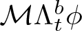 $\mathcal{M}\Lambda^{b}_{t}\phi$ yields
 \begin{equation}
\begin{aligned}
\langle \partial_{t}\Lambda^{b}_{t}\phi+y\partial_{x}\Lambda^{b}_{t}\phi-\mu\partial_{yy} \Lambda^{b}_{t}\phi, \mathcal{M} \Lambda^{b}_{t}\phi\rangle =\langle \Lambda^{b}_{t}(-u\cdot \nabla \phi), \mathcal{M} \Lambda^{b}_{t}\phi\rangle:=H.
\end{aligned}
\end{equation}
According to the properties of multiplier  $\mathcal{M} $ and (1.7), we have
 \begin{equation}
\begin{aligned}
LHS~~ of~~ (3.1)\geqslant & \frac{1}{2}\frac{d}{dt}\|\mathcal{M}^{b}_{t}\phi\|_{L^{2}}^{2}+\frac{1}{2}\|\mathcal{M}^{b}_{t}|D_{x}|(-\Delta)^{-\frac{1}{2}}\phi\|_{L^{2}}^{2}\\
&+\frac{1}{2}\mu\|\mathcal{M}^{b}_{t}\partial_{y}\phi\|_{L^{2}}^{2}+\frac{1}{8}\varpi^{\frac{1}{3}}\|\mathcal{M}^{b}_{t}\vert D_{x}\vert^{\frac{1}{3}}\phi\|_{L^{2}}^{2}.
\end{aligned}
\end{equation}
Then we estimate the nonlinear terms. By  ${\rm div}\,u=0$ and
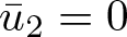 $\bar{u}_{2}=0$, we arrive at
 \begin{equation*}
\begin{aligned}
H&=\langle \mathcal{M}^{b}_{t}(u\cdot \nabla \phi)-u\cdot \nabla(\mathcal{M}^{b}_{t}\phi), \mathcal{M}^{b}_{t}\phi\rangle\\
&=\langle \mathcal{M}^{b}_{t}(\bar{u}_{1}\partial_{x} \phi)-\bar{u}_{1}\partial_{x} (\mathcal{M}^{b}_{t}\phi), \mathcal{M}^{b}_{t}\phi\rangle+\langle \mathcal{M}^{b}_{t}(u_{1}^{\neq}\partial_{x} \phi)-u_{1}^{\neq}\partial_{x} (\mathcal{M}^{b}_{t}\phi), \mathcal{M}^{b}_{t}\phi\rangle\\
&\ \ \ \ +\langle \mathcal{M}^{b}_{t}(u_{2}^{\neq}\partial_{y} \phi)-u_{2}^{\neq}\partial_{y} (\mathcal{M}^{b}_{t}\phi), \mathcal{M}^{b}_{t}\phi\rangle\\
&:=H_{1}+H_{2}+H_{3}.
\end{aligned}
\end{equation*}
To estimate  $H_{1}$, by Plancherel’s formula, we deduce
 \begin{align*}
H_{1} &:=\sum_{k\neq0}\iint(\mathcal{M}^{b}_{t}(k,\xi)-\mathcal{M}^{b}_{t}(k,\xi-\eta))\hat{u}_{1}(0,\eta)\cdot ik\hat{\phi}(k,\xi-\eta)\\
&\qquad\cdot\mathcal{M}^{b}_{t}(k,\xi)\overline{\hat{\phi}(k,\xi)}d\xi d\eta.
\end{align*}
By the differential mean-value theorem, there holds
 \begin{equation*}
\begin{aligned}
H_{1}
&\leqslant C\sum_{k\neq 0}\iint(\varpi^{\frac{1}{3}}|k|^{\frac{2}{3}}+\frac{|k|}{(k^{2}+\xi^{2})^{\frac{1}{2}}}+\frac{|k|}{(k^{2}+(\xi-\eta)^{2})^{\frac{1}{2}}})(\Lambda^{b}_{t}(0,\xi)\\
&\quad +\Lambda^{b}_{t}(k,\xi-\eta))\times|\hat{\omega}(0,\eta)|| \hat{\phi}(k,\xi-\eta)||\mathcal{M}^{b}_{t}(k,\xi)\overline{\hat{\phi}(k,\xi)}|d\xi d\eta.
\end{aligned}
\end{equation*}
Hence, by Young’s convolution inequality, we obtain
 \begin{equation}
\begin{aligned}
H_{1}
\leqslant C(\varpi^{\frac{1}{3}}\|\Lambda^{b}_{t}\bar{\omega}\|_{L^{2}}\|\Lambda^{b}_{t}|D_{x}|^{\frac{1}{3}}\phi\|_{L^{2}}^{2}+\|\Lambda^{b}_{t}\bar{\omega}\|_{L^{2}}\|\Lambda^{b}_{t}|D_{x}|(-\Delta)^{-\frac{1}{2}}\phi\|_{L^{2}}\|\Lambda^{b}_{t}\phi^{\neq}\|_{L^{2}}).
\end{aligned}
\end{equation}
Then we estimate  $H_{2}$. By Plancherel’s formula, we derive
 \begin{equation*}
\begin{aligned}
H_{2}
&:=\sum_{k,l}\iint(\mathcal{M}^{b}_{t}(k,\xi)-\mathcal{M}^{b}_{t}(l,\eta))\hat{u}_{1}^{\neq}(k-l,\xi-\eta)\cdot il\hat{\phi}(l,\eta)\cdot\mathcal{M}^{b}_{t}(k,\xi)\overline{\hat{\phi}(k,\xi)}d\xi d\eta.
\end{aligned}
\end{equation*}
According to the different properties of frequency spaces  $A_{1}$ and
 $A_{2}$, one has
 \begin{equation*}
\begin{aligned}
H_{21}
\leqslant C\sum_{k,l\in A_{1}}\iint(&\Lambda^{b}_{t}(l,\eta)+\Lambda^{b}_{t}(k-l,\xi-\eta))(|k-l|+\varpi^{-\frac{1}{6}}|l|^{\frac{1}{3}}|k|^{\frac{1}{3}})\\
&\times|\hat{u}_{1}^{\neq}(k-l,\xi-\eta)||\hat{\phi}^{\neq}(l,\eta)||\mathcal{M}^{b}_{t}(k,\xi)\overline{\hat{\phi}(k,\xi)}|d\xi d\eta.
\end{aligned}
\end{equation*}
By Lemma 2.1, we have
 \begin{equation}
\begin{aligned}
H_{21}
&\leqslant C(\|\Lambda^{b}_{t}\partial_{x}u_{1}\|_{L^{2}}\|\Lambda^{b}_{t}\phi^{\neq}\|_{L^{2}}\|\Lambda^{b}_{t}\phi\|_{L^{2}}+\varpi^{-\frac{1}{6}}\|\Lambda^{b}_{t}u_{1}^{\neq}\|_{L^{2}}\|\Lambda^{b}_{t}|D_{x}|^{\frac{1}{3}}\phi\|_{L^{2}}^{2}).
\end{aligned}
\end{equation}
And for the second one, by Taylor’s formula and the definition of  $\mathcal{M}$, we get
 \begin{equation*}
\begin{aligned}
H_{22}
\leqslant C\sum_{k,l\in A_{2}}\iint(&\Lambda^{b}_{t}(l,\eta)+\Lambda^{b}_{t}(k-l,\xi-\eta))(\varpi^{\frac{1}{3}}|k|^{-\frac{1}{3}}|l|+1+\varpi^{\frac{1}{2}}|\eta|)\\
&\times|\hat{\omega}^{\neq}(k-l,\xi-\eta)||\hat{\phi}^{\neq}(l,\eta)||\mathcal{M}^{b}_{t}(k,\xi)\overline{\hat{\phi}(k,\xi)}|d\xi d\eta\\
\leqslant C\sum_{k,l\in A_{2}}\iint(&\Lambda^{b}_{t}(l,\eta)+\Lambda^{b}_{t}(k-l,\xi-\eta))(\varpi^{\frac{1}{3}}|k|^{\frac{1}{3}}|l|^{\frac{1}{3}}+\varpi^{\frac{2}{3}}|k|^{\frac{1}{3}}|\eta|)\\
&\times|\hat{\omega}^{\neq}(k-l,\xi-\eta)||\hat{\phi}^{\neq}(l,\eta)||\mathcal{M}^{b}_{t}(k,\xi)\overline{\hat{\phi}(k,\xi)}|d\xi d\eta.
\end{aligned}
\end{equation*}
By Lemma 2.1, it holds that
 \begin{equation}
\begin{aligned}
H_{22}\leqslant C(\varpi^{\frac{1}{3}}\|\Lambda^{b}_{t}\omega\|_{L^{2}}\|\Lambda^{b}_{t}|D_{x}|^{\frac{1}{3}}\phi\|_{L^{2}}^{2}+\varpi^{\frac{2}{3}}\|\Lambda^{b}_{t}\omega\|_{L^{2}}\|\Lambda^{b}_{t}|D_{x}|^{\frac{1}{3}}\phi\|_{L^{2}}\|\Lambda^{b}_{t}\partial_{y}\phi\|_{L^{2}}) .
\end{aligned}
\end{equation}
Hence, combining (3.4) and (3.5) yields
 \begin{equation}
\begin{aligned}
H_{2}
\leqslant&
\,\,C\|\Lambda^{b}_{t}\omega\|_{L^{2}}(\varpi^{-\frac{1}{6}}\|\Lambda^{b}_{t}|D_{x}|^{\frac{1}{3}}\phi\|_{L^{2}}^{2}+\varpi^{\frac{2}{3}}\|\Lambda^{b}_{t}|D_{x}|^{\frac{1}{3}}\phi\|_{L^{2}}\|\Lambda^{b}_{t}\partial_{y}\phi\|_{L^{2}})\\
&\ \ \ \ \ \ +C\|\Lambda^{b}_{t}\partial_{x}u_{1}\|_{L^{2}}\|\Lambda^{b}_{t}\phi^{\neq}\|_{L^{2}}\|\Lambda^{b}_{t}\phi\|_{L^{2}}.
\end{aligned}
\end{equation}
Next, estimate  $H_{3}$. By Plancherel’s formula, we arrive at
 \begin{equation*}
\begin{aligned}
H_{3}
:=\sum_{k,l}\iint(&\mathcal{M}^{b}_{t}(k,\xi)-\mathcal{M}^{b}_{t}(k-l,\xi-\eta))\hat{u}_{2}^{\neq}(l,\eta)\cdot i(\xi-\eta)\hat{\phi}(k-l,\xi-\eta)\\
&\times\mathcal{M}^{b}_{t}(k,\xi)\overline{\hat{\phi}(k,\xi)}d\xi d\eta.
\end{aligned}
\end{equation*}
By Lemma 2.1 and the boundedness of multiplier  $\mathcal{M}$, we deduce
 \begin{equation}
\begin{aligned}
H_{3}
&\leqslant C\|\Lambda^{b}_{t}u_{2}^{\neq}\|_{L^{2}}\|\Lambda^{b}_{t}\partial_{y}\phi\|_{L^{2}}\|\Lambda^{b}_{t}\phi\|_{L^{2}}\\
&\leqslant C\|\Lambda^{b}_{t}|D_{x}|(-\Delta)^{-\frac{1}{2}}\omega^{\neq}\|_{L^{2}}\|\Lambda^{b}_{t}\partial_{y}\phi\|_{L^{2}}\|\Lambda^{b}_{t}\phi\|_{L^{2}}.
\end{aligned}
\end{equation}
Combining (3.3), (3.6), and (3.7), we have
 \begin{equation}
\begin{aligned}
H
&\leqslant C\|\Lambda^{b}_{t}\omega\|_{L^{2}}(\varpi^{\frac{2}{3}}\|\Lambda^{b}_{t}|D_{x}|^{\frac{1}{3}}\phi\|_{L^{2}}\|\Lambda^{b}_{t}\partial_{y}\phi\|_{L^{2}}+\|\Lambda^{b}_{t}|D_{x}|(-\Delta)^{-\frac{1}{2}}\phi\|_{L^{2}}\|\Lambda^{b}_{t}\phi^{\neq}\|_{L^{2}})\\
&\ \ \ \ \ \ +C\|\Lambda^{b}_{t}\phi\|_{L^{2}}\|\Lambda^{b}_{t}|D_{x}|(-\Delta)^{-\frac{1}{2}}\omega^{\neq}\|_{L^{2}}(\|\Lambda^{b}_{t}\phi^{\neq}\|_{L^{2}}+ \|\Lambda^{b}_{t}\partial_{y}\phi\|_{L^{2}})\\
&\ \ \ \ \ \ + C\varpi^{-\frac{1}{6}}\|\Lambda^{b}_{t}\omega\|_{L^{2}}\|\Lambda^{b}_{t}|D_{x}|^{\frac{1}{3}}\phi\|_{L^{2}}^{2}.
\end{aligned}
\end{equation}
Therefore,
 \begin{align}
&\frac{d}{dt}\|\mathcal{M}^{b}_{t}\phi\|_{L^{2}}^{2}+\mu\|\mathcal{M}^{b}_{t}\partial_{y}\phi\|_{L^{2}}^{2}+\varpi^{\frac{1}{3}}\|\mathcal{M}^{b}_{t}\vert D_{x}\vert^{\frac{1}{3}}\phi\|_{L^{2}}^{2}+\|\mathcal{M}^{b}_{t}|D_{x}|(-\Delta)^{-\frac{1}{2}}\phi\|_{L^{2}}^{2}\nonumber\\
&\qquad\leqslant C\|\Lambda^{b}_{t}\omega\|_{L^{2}}(\varpi^{\frac{2}{3}}\|\Lambda^{b}_{t}|D_{x}|^{\frac{1}{3}}\phi\|_{L^{2}}\|\Lambda^{b}_{t}\partial_{y}\phi\|_{L^{2}}\nonumber\\
&\quad+\|\Lambda^{b}_{t}|D_{x}|(-\Delta)^{-\frac{1}{2}}\phi\|_{L^{2}}\|\Lambda^{b}_{t}\phi^{\neq}\|_{L^{2}})\nonumber\\
&\quad +C\|\Lambda^{b}_{t}\phi\|_{L^{2}}\|\Lambda^{b}_{t}|D_{x}|(-\Delta)^{-\frac{1}{2}}\omega^{\neq}\|_{L^{2}}(\|\Lambda^{b}_{t}\phi^{\neq}\|_{L^{2}}+ \|\Lambda^{b}_{t}\partial_{y}\phi\|_{L^{2}})\nonumber\\
&\quad+ C\varpi^{-\frac{1}{6}}\|\Lambda^{b}_{t}\omega\|_{L^{2}}\|\Lambda^{b}_{t}|D_{x}|^{\frac{1}{3}}\phi\|_{L^{2}}^{2}.
\end{align}
Based on the result of Theorem 1.1, notice that
 \begin{align*}
&\|\Lambda^{b}_{t}\omega\|_{L^{\infty}L^{2}} +\varpi^{\frac{1}{2}}\|\Lambda^{b}_{t}\partial_{y}\omega\|_{L^{2}L^{2}}+\varpi^{\frac{1}{6}}\|\Lambda^{b}_{t}\vert D_{x}\vert^{\frac{1}{3}}\omega\|_{L^{2}L^{2}}\\
&\quad +\|\Lambda^{b}_{t}|D_{x}|(-\Delta)^{-\frac{1}{2}}\omega\|_{L^{2}L^{2}}\leqslant C\varepsilon \varpi^{\frac{1}{2}},\end{align*}
we deduce from (3.9)
 \begin{align}
&\|\mathcal{M}^{b}_{t}\phi\|_{L^{\infty}L^{2}}^{2}+\mu\|\mathcal{M}^{b}_{t}\partial_{y}\phi\|_{L^{2}L^{2}}^{2}+\varpi^{\frac{1}{3}}\|\mathcal{M}^{b}_{t}\vert D_{x}\vert^{\frac{1}{3}}\phi\|_{L^{2}L^{2}}^{2}+\|\mathcal{M}^{b}_{t}|D_{x}|(-\Delta)^{-\frac{1}{2}}\phi\|_{L^{2}L^{2}}^{2}\nonumber\\
&\qquad \leqslant C\varepsilon \varpi^{\frac{1}{2}}(\varpi^{\frac{2}{3}}\|\Lambda^{b}_{t}|D_{x}|^{\frac{1}{3}}\phi\|_{L^{2}L^{2}}\|\Lambda^{b}_{t}\partial_{y}\phi\|_{L^{2}L^{2}}\nonumber\\
&\quad +\|\Lambda^{b}_{t}|D_{x}|(-\Delta)^{-\frac{1}{2}}\phi\|_{L^{2}L^{2}}\|\Lambda^{b}_{t}\phi^{\neq}\|_{L^{2}L^{2}})+\nonumber\\
&\quad+C\varepsilon \varpi^{\frac{1}{2}}\|\Lambda^{b}_{t}\phi\|_{L^{\infty}L^{2}}(\|\Lambda^{b}_{t}\phi^{\neq}\|_{L^{2}L^{2}}+ \|\Lambda^{b}_{t}\partial_{y}\phi\|_{L^{2}L^{2}})\nonumber\\
&\quad+ C\varepsilon \varpi^{\frac{1}{3}}\|\Lambda^{b}_{t}|D_{x}|^{\frac{1}{3}}\phi\|_{L^{2}L^{2}}^{2}++(2+\pi)\|\phi_{0}\|_{H^{b}}^{2}\nonumber\\
&\qquad\leqslant C\varepsilon \varpi^{\frac{1}{2}}(\varpi^{\frac{2}{3}}\mu^{-\frac{1}{2}}\|\Lambda^{b}_{t}|D_{x}|^{\frac{1}{3}}\phi\|_{L^{2}L^{2}}\mu^{\frac{1}{2}}\|\Lambda^{b}_{t}\partial_{y}\phi\|_{L^{2}L^{2}}\nonumber\\
&\quad+\|\Lambda^{b}_{t}|D_{x}|(-\Delta)^{-\frac{1}{2}}\phi\|_{L^{2}L^{2}}\|\Lambda^{b}_{t}\phi^{\neq}\|_{L^{2}L^{2}})+\nonumber\\
&\quad+C\varepsilon \varpi^{\frac{1}{2}}\|\Lambda^{b}_{t}\phi\|_{L^{\infty}L^{2}}(\|\Lambda^{b}_{t}\phi^{\neq}\|_{L^{2}L^{2}}+ \mu^{-\frac{1}{2}}\mu^{\frac{1}{2}}\|\Lambda^{b}_{t}\partial_{y}\phi\|_{L^{2}L^{2}})\nonumber\\
&\quad + C\varepsilon \varpi^{\frac{1}{3}}\|\Lambda^{b}_{t}|D_{x}|^{\frac{1}{3}}\phi\|_{L^{2}L^{2}}^{2}+\nonumber\\
&\quad+(2+\pi)\|\phi_{0}\|_{H^{b}}^{2}.
\end{align}
Then utilizing the boundedness of  $\mathcal{M}$ and Hölder inequality, one has
 \begin{equation}
\begin{aligned}
&\|\Lambda^{b}_{t}\phi\|_{L^{\infty}L^{2}}^{2}+\mu\|\Lambda^{b}_{t}\partial_{y}\phi\|_{L^{2}L^{2}}^{2}+\varpi^{\frac{1}{3}}\|\Lambda^{b}_{t}\vert D_{x}\vert^{\frac{1}{3}}\phi\|_{L^{2}L^{2}}^{2}+\|\Lambda^{b}_{t}|D_{x}|(-\Delta)^{-\frac{1}{2}}\phi\|_{L^{2}L^{2}}^{2}\\
&\leqslant (2+\pi)\|\phi_{0}\|_{H^{b}}^{2}+C\varepsilon (\varpi^{\frac{1}{2}}\|\Lambda^{b}_{t}|D_{x}|(-\Delta)^{-\frac{1}{2}}\phi\|^{2}_{L^{2}L^{2}}+ \varpi^{\frac{1}{3}}\|\Lambda^{b}_{t}|D_{x}|^{\frac{1}{3}}\phi\|_{L^{2}L^{2}}^{2})\\
&\ \ \ \ \ \ \ \ + C\varepsilon (\|\Lambda^{b}_{t}\phi\|^{2}_{L^{\infty}L^{2}}+\mu\|\Lambda^{b}_{t}\partial_{y}\phi\|^{2}_{L^{2}L^{2}}).
\end{aligned}
\end{equation}
Choosing 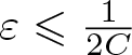 $\varepsilon\leqslant \frac{1}{2C}$, we get
 \begin{align}
&\|\Lambda^{b}_{t}\phi\|_{L^{\infty}L^{2}}^{2}+\mu\|\Lambda^{b}_{t}\partial_{y}\phi\|_{L^{2}L^{2}}^{2}+\varpi^{\frac{1}{3}}\|\Lambda^{b}_{t}\vert D_{x}\vert^{\frac{1}{3}}\phi\|_{L^{2}L^{2}}^{2}\nonumber\\
&\qquad +\|\Lambda^{b}_{t}|D_{x}|(-\Delta)^{-\frac{1}{2}}\phi\|_{L^{2}L^{2}}^{2}\leqslant 11\|\phi_{0}\|_{H^{b}}^{2}.
\end{align}
Hence, the proof of Corollary 1.2 is completed.
Data availability
Since this work is of abstract theoretical nature, no data sets are generated or analysed. One can obtain the relevant materials from the reference list.
Acknowledgements
X. Xu was partially supported by the National Natural Science Foundation of China (Grant Nos. 12571244 and 12171040). J. Wu was partially supported by the National Science Foundation of the United States (Grant Nos. DMS 2104682 and DMS 2309748).
Funding statement
Open Access funding enabled and organized by Beijing Normal University.
Declaration of competing interest
The authors declare that they have no conflict of interest.
Author contributions
All authors contributed to the study conception and design. Material preparation and analysis were performed by C.L., H.W., J.W., and X.X. The first draft of the manuscript was written by H.W., and all authors commented on previous versions of the manuscript. All authors read and approved the final manuscript.
Open Access
This article is licensed under a Creative Commons Attribution 4.0 International License, which permits use, sharing, adaptation, distribution, and reproduction in any medium or format, as long as you give appropriate credit to the original author(s) and the source, provide a link to the Creative Commons licence, and indicate if changes were made. The images or other third-party material in this article are included in the article’s Creative Commons licence, unless indicated otherwise in a credit line to the material. If material is not included in the article’s Creative Commons licence and your intended use is not permitted by statutory regulation or exceeds the permitted use, you will need to obtain permission directly from the copyright holder. To view a copy of this licence, visit http://creativecommons.org/licenses/by/4.0/.