1 Introduction
Collisionless shocks, even at low-Mach numbers, are complicated structures. The majority of the shocks encountered in the heliosphere are fast magnetized shocks, where the shock transition is mainly identified by the rapid increase of the magnetic field (see, e.g. Kennel, Edmiston & Hada Reference Kennel, Edmiston and Hada1985, for a review). The magnetic jump must be accompanied by a drop in fluid speed from super- to submagnetosonic and a jump in the ion and electron density, and by an increase of temperatures of both species. However, it is the magnetic field which is (i) measured with the highest precision, and (ii) serves as the main signature of the shock. Knowledge of the structure of the magnetic profile is of the utmost importance, since the macroscopic magnetic field is the most important factor affecting the particle motion throughout the shock. The primary parameters defining the shock behavior are thought to be the Mach number,
 $M$
(defined below), the angle,
 $\unicode[STIX]{x1D703}$
, between the shock normal and the upstream magnetic field, and the ratio of the upstream kinetic-to-magnetic pressure
 $\unicode[STIX]{x1D6FD}=8\unicode[STIX]{x03C0}p_{u}/B_{u}^{2}$
. Here
 $p_{u}=n_{u}T_{u}$
is the upstream plasma pressure and
 $B_{u}$
is the upstream magnetic field. Hereafter the subscript
 $u$
refers to the upstream values and
 $d$
refers to the downstream parameters. Low-Mach number, low-
 $\unicode[STIX]{x1D6FD}$
shocks are believed to be laminar, that is, to possess an almost monotonic increase of the magnetic field with nearly no magnetic oscillations (Greenstadt et al.
Reference Greenstadt, Scarf, Russell, Formisano and Neugebauer1975; Mellott & Greenstadt Reference Mellott and Greenstadt1984; Farris, Russell & Thomsen Reference Farris, Russell and Thomsen1993). Recently, it was shown that even in very low-Mach number shocks, downstream magnetic oscillations are caused by ion gyration (Balikhin et al.
Reference Balikhin, Zhang, Gedalin, Ganushkina and Pope2008; Ofman et al.
Reference Ofman, Balikhin, Russell and Gedalin2009; Russell et al.
Reference Russell, Jian, Blanco-Cano and Luhmann2009; Kajdič et al.
Reference Kajdič, Blanco-Cano, Aguilar-Rodriguez, Russell, Jian and Luhmann2012; Ofman & Gedalin Reference Ofman and Gedalin2013; Gedalin, Friedman & Balikhin Reference Gedalin, Friedman and Balikhin2015a
). Low-Mach number shocks also often exhibit magnetic oscillations upstream of the ramp (Balikhin et al.
Reference Balikhin, Pokhotelov, Walker and André2003; Blanco-Cano, Omidi & Russell Reference Blanco-Cano, Omidi and Russell2006; Wilson et al.
Reference Wilson, Cattell, Kellogg, Goetz, Kersten, Hanson, MacGregor and Kasper2007, Reference Wilson, Cattell, Kellogg, Goetz, Kersten, Kasper, Szabo and Meziane2009; Ramírez Vélez et al.
Reference Ramírez Vélez, Blanco-Cano, Aguilar-Rodriguez, Russell, Kajdič, Jian and Luhmann2012; Blanco-Cano et al.
Reference Blanco-Cano, Kajdič, Aguilar-Rodriguez, Russell, Jian and Luhmann2013, Reference Blanco-Cano, Kajdič, Aguilar-Rodriguez, Russell, Jian and Luhmann2016; Wilson et al.
Reference Wilson III, Koval, Szabo, Stevens, Kasper, Cattell and Krasnoselskikh2017), typically identified as low-frequency electromagnetic whistlers (Ramírez Vélez et al.
Reference Ramírez Vélez, Blanco-Cano, Aguilar-Rodriguez, Russell, Kajdič, Jian and Luhmann2012). Whistler generation is quite typical for supercritical shocks (Walker, Balikhin & Nozdrachev Reference Walker, Balikhin and Nozdrachev1999; Scholer & Burgess Reference Scholer and Burgess2007; Hull et al.
Reference Hull, Muschietti, Oka, Larson, Mozer, Chaston, Bonnell and Hospodarsky2012; Wilson et al.
Reference Wilson, Koval, Szabo, Breneman, Cattell, Goetz, Kellogg, Kersten, Kasper and Maruca2012). Often these whistlers propagate at an angle to the shock normal and possibly precede the formation of ripples in supercritical shocks (Lowe & Burgess Reference Lowe and Burgess2003; Burgess & Scholer Reference Burgess and Scholer2007; Lobzin et al.
Reference Lobzin, Krasnoselskikh, Musatenko and de Wit2008; Johlander et al.
Reference Johlander, Schwartz, Vaivads, Khotyaintsev, Gingell, Peng, Markidis, Lindqvist, Ergun and Marklund2016; Gingell et al.
Reference Gingell, Schwartz, Burgess, Johlander, Russell, Burch, Ergun, Fuselier, Gershman and Giles2017). It was also suggested that at higher Mach numbers, whistler generation evolves into strong non-stationarity of the shock front, known as reformation (Walker et al.
Reference Walker, Balikhin and Nozdrachev1999; Krasnoselskikh et al.
Reference Krasnoselskikh, Lembège, Savoini and Lobzin2002; Scholer & Burgess Reference Scholer and Burgess2007; Lobzin et al.
Reference Lobzin, Krasnoselskikh, Musatenko and de Wit2008; Lembège et al.
Reference Lembège, Savoini, Hellinger and Trávníček2009; Krasnoselskikh, Balikhin & Walker Reference Krasnoselskikh, Balikhin and Walker2013; Sulaiman et al.
Reference Sulaiman, Masters, Dougherty, Burgess, Fujimoto and Hospodarsky2015). In high-Mach number shocks, whistlers may be also generated by instabilities in the foot (Riquelme & Spitkovsky Reference Riquelme and Spitkovsky2011; Wilson et al.
Reference Wilson, Koval, Szabo, Breneman, Cattell, Goetz, Kellogg, Kersten, Kasper and Maruca2012). In low-Mach number shocks with no foot and/or reflected ions this option is less plausible although cannot be completely excluded. It is the general understanding that stationarity of even low-Mach number shocks requires the presence of some dissipation, presumably in the form of resistivity. The de facto standard semiqualitative description of the shock front suggests transformation of a soliton solution into a shock-like profile when dispersion is accompanied with weak dissipation (Sagdeev Reference Sagdeev1966). Since then most of the effort was devoted to the stationary shock description. The only time-dependent gradient catastrophe model was proposed by Krasnoselskikh et al. (Reference Krasnoselskikh, Lembège, Savoini and Lobzin2002) for reformation of strong shocks. It was shown that in the presence of weak resistive dissipation, shock-like solutions do exist in one-dimensional two-fluid quasineutral approximation (Gedalin Reference Gedalin1998), while without dissipation there are no solutions with different asymptotic values of the magnetic field. The appearance of downstream magnetic oscillations is a kinetic effect (Ofman et al.
Reference Ofman, Balikhin, Russell and Gedalin2009; Gedalin et al.
Reference Gedalin, Friedman and Balikhin2015a
) and cannot be properly described within the widely accepted single polytropic two-fluid theory. Yet, upstream of the ramp the two-fluid approach is still a good approximation. It was shown that even if restricting for the upstream region only, stationary solutions with decaying oscillations exist only if dissipation is invoked (Gedalin, Kushinsky & Balikhin Reference Gedalin, Kushinsky and Balikhin2015b
). This brings us to the conclusion that even low-Mach shocks may be intrinsically non-stationary and generate upstream propagating whistler wave trains. Weakly nonlinear weakly dispersive waves are typically described by the Korteveg-de-Vries equation (KdV) (Karpman Reference Karpman1975; Ablowitz Reference Ablowitz2011). The asymptotic behavior of the initial discontinuity in the KdV has been studied using the Witham method (Gurevich & Pitayevsky Reference Gurevich and Pitayevsky1974) and by direct numerical integration (Ablowitz, Baldwin & Hoefer Reference Ablowitz, Baldwin and Hoefer2009; Ablowitz & Baldwin Reference Ablowitz and Baldwin2013). However, in the physically meaningful situation, an initially smooth profile steepens and wave train generation is expected to prevent discontinuity formation. The physically interesting stage, to be compared with observations, is not the asymptotic state but the transient one, when also taking into account the variability of the ambient conditions. In general, one-dimensional time-dependent nonlinear waves in two-fluid theory are described by a set of equations which are more complicated than the KdV equation (Gedalin Reference Gedalin1993, Reference Gedalin1994). In the present paper we derive the time-dependent equations for one-dimensional waves in two-fluid theory with resistive dissipation included. We reduce these equations to a single KdV–Burgers equation and analyze it numerically. We show that in the case of sufficiently weak dissipation an initially smooth profile with different asymptotic values of the magnetic field steepens to an intrinsically non-stationary shock, generating upstream wave trains.
2 Basic equations
The analysis will be done within two-fluid plasma theory with massless electrons, since in low-Mach number shocks the typical spatial scales are often much larger than the electron inertial length and the typical temporal scales are much larger than the electron gyroperiod or inverse electron plasma frequency (see, however, Wilson et al.
Reference Wilson III, Koval, Szabo, Stevens, Kasper, Cattell and Krasnoselskikh2017). For the same reason quasineutrality,
 $n_{e}=n_{i}=n$
, is maintained with high precision. The speeds are well below the speed of light, so that the displacement current is negligible. We also assume that the system is one-dimensional, that is, all plasma variables and fields depend only on the coordinate
 $x$
along the shock normal and on time
 $t$
. With these approximations the two-fluid equations take the form
 $$\begin{eqnarray}\displaystyle & \unicode[STIX]{x2202}_{t}n+\unicode[STIX]{x2202}_{x}(nv_{x})=0, & \displaystyle\end{eqnarray}$$
 $$\begin{eqnarray}\displaystyle & nm_{i}\left(\unicode[STIX]{x2202}_{t}v_{x}+v_{x}\unicode[STIX]{x2202}_{x}v_{x}\right)=ne\left(E_{x}+\hat{\boldsymbol{x}}\boldsymbol{\cdot }(\boldsymbol{v}_{i}\times \boldsymbol{B})/c\right)-\unicode[STIX]{x2202}_{x}p_{i}, & \displaystyle\end{eqnarray}$$
 $$\begin{eqnarray}\displaystyle & 0=-en\left(E_{x}+\hat{\boldsymbol{x}}\boldsymbol{\cdot }(\boldsymbol{v}_{e}\times \boldsymbol{B})/c\right)-\unicode[STIX]{x2202}_{x}p_{e}, & \displaystyle\end{eqnarray}$$
 $$\begin{eqnarray}\displaystyle & \hspace{-6.0pt}nm_{i}\left(\unicode[STIX]{x2202}_{t}\boldsymbol{v}_{i\bot }+v_{x}\unicode[STIX]{x2202}_{x}\boldsymbol{v}_{i\bot }\right)=ne\left(\boldsymbol{E}_{\bot }+v_{x}\hat{\boldsymbol{x}}\times \boldsymbol{B}_{\bot }/c+B_{x}\boldsymbol{v}_{i\bot }\times \hat{\boldsymbol{x}}/c\right)-n\unicode[STIX]{x1D708}(\boldsymbol{v}_{i\bot }-\boldsymbol{v}_{e\bot }), & \displaystyle\end{eqnarray}$$
 $$\begin{eqnarray}\displaystyle & 0=-en\left(\boldsymbol{E}_{\bot }+v_{x}\hat{\boldsymbol{x}}\times \boldsymbol{B}_{\bot }/c+B_{x}\boldsymbol{v}_{e\bot }\times \hat{\boldsymbol{x}}/c\right)-n\unicode[STIX]{x1D708}(\boldsymbol{v}_{e\bot }-\boldsymbol{v}_{i\bot }), & \displaystyle\end{eqnarray}$$
 $$\begin{eqnarray}\displaystyle & c\unicode[STIX]{x2202}_{x}(\hat{\boldsymbol{x}}\times \boldsymbol{B}_{\bot })=4\unicode[STIX]{x03C0}ne(\boldsymbol{v}_{i\bot }-\boldsymbol{v}_{e\bot }), & \displaystyle\end{eqnarray}$$
 $$\begin{eqnarray}\displaystyle & \unicode[STIX]{x2202}_{t}\boldsymbol{B}_{\bot }=-c\unicode[STIX]{x2202}_{x}(\hat{\boldsymbol{x}}\times \boldsymbol{E}_{\bot }), & \displaystyle\end{eqnarray}$$
 $$\begin{eqnarray}\displaystyle & B_{x}=\text{const.},\quad v_{ex}=v_{ix}=v_{x}. & \displaystyle\end{eqnarray}$$
Here
 $n$
,
 $v_{x}$
, and
 $\boldsymbol{v}_{\bot }$
are the ion density and velocity,
 $B_{x}$
and
 $\boldsymbol{B}_{\bot }$
are the magnetic field components, while
 $E_{x}$
and
 $\boldsymbol{E}_{\bot }$
are the electric field components. The subscript
 $\bot$
denotes components perpendicular to the shock normal:
 $\boldsymbol{v}_{\bot }=(v_{y},v_{z})$
,
 $\boldsymbol{B}_{\bot }=(B_{y},B_{z})$
,
 $\boldsymbol{E}_{\bot }=(E_{y},E_{z})$
. Here
 $\bot$
refers to the direction
 $\hat{\boldsymbol{x}}$
. We shall assume that
 $p_{e}$
and
 $p_{i}$
are functions of the density only. The derivation essentially follows Gedalin (Reference Gedalin1993) except that here we do not switch to Lagrangian variables. The last term in (2.4) and (2.5) describes the friction (momentum exchange) between the two species while conserving the total momentum. Indeed, the following conservation laws can be easily derived:
 $$\begin{eqnarray}\displaystyle & \unicode[STIX]{x2202}_{t}n+\unicode[STIX]{x2202}_{x}(nv_{x})=0, & \displaystyle\end{eqnarray}$$
 $$\begin{eqnarray}\displaystyle & \displaystyle \unicode[STIX]{x2202}_{t}(nm_{i}v_{x})+\unicode[STIX]{x2202}_{x}\left(nm_{i}v_{x}^{2}+p+\frac{B_{\bot }^{2}}{8\unicode[STIX]{x03C0}}\right)=0, & \displaystyle\end{eqnarray}$$
 $$\begin{eqnarray}\displaystyle & \displaystyle \unicode[STIX]{x2202}_{t}(nm_{i}\boldsymbol{v}_{i\bot })+\unicode[STIX]{x2202}_{x}\left(nm_{i}v_{x}\boldsymbol{v}_{i\bot }-\frac{B_{x}\boldsymbol{B}_{\bot }}{4\unicode[STIX]{x03C0}}\right)=0, & \displaystyle\end{eqnarray}$$
which are the particle number and the momentum conservation and
 $p=p_{i}+p_{e}$
. Equations (2.5) and (2.6) give
 $$\begin{eqnarray}\displaystyle & \displaystyle c(\hat{\boldsymbol{x}}\times \boldsymbol{E}_{\bot })=v_{x}\boldsymbol{B}_{\bot }-B_{x}\boldsymbol{v}_{i\bot }+\frac{cB_{x}}{4\unicode[STIX]{x03C0}ne}\unicode[STIX]{x2202}_{x}(\hat{\boldsymbol{x}}\times \boldsymbol{B}_{\bot })-\frac{c^{2}\unicode[STIX]{x1D708}}{4\unicode[STIX]{x03C0}ne^{2}}\unicode[STIX]{x2202}_{x}\boldsymbol{B}_{\bot } & \displaystyle\end{eqnarray}$$
so that (2.7) takes the form
 $$\begin{eqnarray}\displaystyle & \displaystyle \unicode[STIX]{x2202}_{t}\boldsymbol{B}_{\bot }+\unicode[STIX]{x2202}_{x}(v_{x}\boldsymbol{B}_{\bot }-B_{x}\boldsymbol{v}_{i\bot })+\unicode[STIX]{x2202}_{x}\left(\frac{cB_{x}}{4\unicode[STIX]{x03C0}ne}\unicode[STIX]{x2202}_{x}(\hat{\boldsymbol{x}}\times \boldsymbol{B}_{\bot })-\frac{c^{2}\unicode[STIX]{x1D708}}{4\unicode[STIX]{x03C0}ne^{2}}\unicode[STIX]{x2202}_{x}\boldsymbol{B}_{\bot }\right)=0. & \displaystyle\end{eqnarray}$$
Let us choose some point as a reference point, denoted from here onward by the subscript ‘0’. It is always possible to switch to a reference frame such that in this reference point
 $\boldsymbol{v}_{0,i\bot }=0$
. It is always possible to rotate to a coordinate system around axis
 $x$
in such a way so that in the reference point
 $B_{0,y}=0$
. We shall denote the other variables in the reference point as follows:
 $n=n_{0}$
,
 $B_{0,x}=B_{0}\cos \unicode[STIX]{x1D703}$
,
 $B_{0,z}=B_{0}\sin \unicode[STIX]{x1D703}$
and
 $p=p_{0}$
.
We further define
 $$\begin{eqnarray}\displaystyle & & \displaystyle \displaystyle v_{A}^{2}=\frac{B_{0}^{2}}{4\unicode[STIX]{x03C0}n_{0}m_{i}},\quad \unicode[STIX]{x1D714}_{pi}^{2}=\frac{4\unicode[STIX]{x03C0}n_{0}e^{2}}{m_{i}},\quad \unicode[STIX]{x1D6FA}=\frac{eB_{0}}{m_{i}c},\quad \unicode[STIX]{x1D6FD}=\frac{8\unicode[STIX]{x03C0}p_{0}}{B_{0}^{2}},\quad M=\frac{v_{0}}{v_{A}}.\end{eqnarray}$$
It is convenient to introduce the normalized variables as follows:
 $$\begin{eqnarray}\displaystyle & \displaystyle T=\unicode[STIX]{x1D6FA}t,\quad X=\frac{\unicode[STIX]{x1D714}_{pi}x}{c},\quad N=\frac{n}{n_{0}},\quad v=\frac{v_{x}}{v_{A}}, & \displaystyle\end{eqnarray}$$
 $$\begin{eqnarray}\displaystyle & \displaystyle \boldsymbol{u}=\frac{\boldsymbol{v}_{i\bot }}{v_{A}},\quad \boldsymbol{b}=\frac{\boldsymbol{B}_{\bot }}{B_{0}}. & \displaystyle\end{eqnarray}$$
We shall also assume the polytropic state equation
 $p/n^{\unicode[STIX]{x1D6FE}}=\text{const}$
. In the normalized form the equations are written as follows:
 $$\begin{eqnarray}\displaystyle & \unicode[STIX]{x2202}_{T}N+\unicode[STIX]{x2202}_{X}(Nv)=0, & \displaystyle\end{eqnarray}$$
 $$\begin{eqnarray}\displaystyle & \displaystyle \unicode[STIX]{x2202}_{T}(Nv)+\unicode[STIX]{x2202}_{X}\left(Nv^{2}+\frac{\unicode[STIX]{x1D6FD}N^{\unicode[STIX]{x1D6FE}}+b^{2}}{2}\right)=0, & \displaystyle\end{eqnarray}$$
 $$\begin{eqnarray}\displaystyle & \unicode[STIX]{x2202}_{T}(N\boldsymbol{u})+\unicode[STIX]{x2202}_{X}\left(Nv\boldsymbol{u}-\cos \unicode[STIX]{x1D703}\boldsymbol{b}\right)=0, & \displaystyle\end{eqnarray}$$
 $$\begin{eqnarray}\displaystyle & \unicode[STIX]{x2202}_{T}\boldsymbol{b}+\unicode[STIX]{x2202}_{X}(v\boldsymbol{b}-\cos \unicode[STIX]{x1D703}\boldsymbol{u})+\cos \unicode[STIX]{x1D703}\unicode[STIX]{x2202}_{X}(N^{-1}\unicode[STIX]{x2202}_{X}(\hat{\boldsymbol{x}}\times \boldsymbol{b}))-\unicode[STIX]{x1D707}\unicode[STIX]{x2202}_{X}(N^{-1}\unicode[STIX]{x2202}_{X}\boldsymbol{b})=0. & \displaystyle\end{eqnarray}$$
It is useful to write down (2.17)–(2.19) using the variables
 $J=Nv$
, and
 $\boldsymbol{W}=n\boldsymbol{u}$
:
 $$\begin{eqnarray}\displaystyle & \unicode[STIX]{x2202}_{T}N+\unicode[STIX]{x2202}_{X}J=0 & \displaystyle\end{eqnarray}$$
 $$\begin{eqnarray}\displaystyle & \displaystyle \unicode[STIX]{x2202}_{T}J+\unicode[STIX]{x2202}_{X}\left(\frac{J^{2}}{N}+\frac{\unicode[STIX]{x1D6FD}N^{\unicode[STIX]{x1D6FE}}+b^{2}}{2}\right)=0 & \displaystyle\end{eqnarray}$$
 $$\begin{eqnarray}\displaystyle & \displaystyle \unicode[STIX]{x2202}_{T}\boldsymbol{W}+\unicode[STIX]{x2202}_{X}\left(\frac{\boldsymbol{W}}{N}-\cos \unicode[STIX]{x1D703}\boldsymbol{b}\right)=0. & \displaystyle\end{eqnarray}$$
Gedalin (Reference Gedalin1993) derive two equations for the two components of the perpendicular magnetic field. These equations contain second-order time derivatives and are written in Lagrangian variables. Here we use a different path expressing the equations as conservation laws, since conservation laws are of utmost importance for shocks. Indeed, in the stationary case the conservation laws provide algebraic constraints connecting the plasma and field variables.
3 Stationary states
If there is no time dependence we arrive at the following conservation laws
 $$\begin{eqnarray}\displaystyle & J=M, & \displaystyle\end{eqnarray}$$
 $$\begin{eqnarray}\displaystyle & \displaystyle \frac{M^{2}}{N}+\frac{\unicode[STIX]{x1D6FD}N^{\unicode[STIX]{x1D6FE}}+b_{y}^{2}+b_{z}^{2}}{2}=M^{2}+\frac{\unicode[STIX]{x1D6FD}+\sin ^{2}\unicode[STIX]{x1D703}}{2}, & \displaystyle\end{eqnarray}$$
 $$\begin{eqnarray}\displaystyle & \displaystyle \frac{W_{y}}{N}-\cos \unicode[STIX]{x1D703}b_{y}=0, & \displaystyle\end{eqnarray}$$
 $$\begin{eqnarray}\displaystyle & \displaystyle \frac{W_{z}}{N}-\cos \unicode[STIX]{x1D703}b_{z}=-\cos \unicode[STIX]{x1D703}\sin \unicode[STIX]{x1D703}, & \displaystyle\end{eqnarray}$$
while the remaining equations for
 $b_{y}$
and
 $b_{z}$
take the form
 $$\begin{eqnarray}\displaystyle & Mb_{y}-\cos \unicode[STIX]{x1D703}W_{y}-\cos \unicode[STIX]{x1D703}\unicode[STIX]{x2202}_{X}b_{z}-\unicode[STIX]{x1D707}\unicode[STIX]{x2202}_{X}b_{y}=C_{y}, & \displaystyle\end{eqnarray}$$
 $$\begin{eqnarray}\displaystyle & Mb_{z}-\cos \unicode[STIX]{x1D703}W_{z}+\cos \unicode[STIX]{x1D703}\unicode[STIX]{x2202}_{X}b_{y}-\unicode[STIX]{x1D707}\unicode[STIX]{x2202}_{X}b_{z}=C_{z}, & \displaystyle\end{eqnarray}$$
where the constants
 $C_{y}$
and
 $C_{z}$
should be determined by additional conditions in the reference point. Since we are particularly interested in solutions which asymptotically converge to an uniform state, we take the reference point at
 $x\rightarrow \pm \infty$
and assume that all derivatives vanish there, that is,
 $C_{y}=0$
and
 $C_{z}=\sin \unicode[STIX]{x1D703}$
. Eventually, one has
 $$\begin{eqnarray}\displaystyle & \displaystyle \frac{1}{N}+\frac{\unicode[STIX]{x1D6FD}N^{\unicode[STIX]{x1D6FE}}}{2M^{2}}+\frac{b^{2}}{2M^{2}}=1+\frac{\unicode[STIX]{x1D6FD}+\sin ^{2}\unicode[STIX]{x1D703}}{2M^{2}}, & \displaystyle\end{eqnarray}$$
 $$\begin{eqnarray}\displaystyle & b_{y}(M^{2}-N\cos ^{2}\unicode[STIX]{x1D703})-\cos \unicode[STIX]{x1D703}\unicode[STIX]{x2202}_{X}b_{z}-\unicode[STIX]{x1D707}\unicode[STIX]{x2202}_{X}b_{y}=0, & \displaystyle\end{eqnarray}$$
 $$\begin{eqnarray}\displaystyle & b_{z}(M^{2}-N\cos ^{2}\unicode[STIX]{x1D703})+\cos \unicode[STIX]{x1D703}\unicode[STIX]{x2202}_{X}b_{y}-\unicode[STIX]{x1D707}\unicode[STIX]{x2202}_{X}b_{z}=N\sin \unicode[STIX]{x1D703}(M^{2}-\cos ^{2}\unicode[STIX]{x1D703}). & \displaystyle\end{eqnarray}$$
We start with the analysis of the stationary point by linearizing the equations for
 $N=1+\unicode[STIX]{x1D6FF}N$
,
 $b_{z}=\sin \unicode[STIX]{x1D703}+\unicode[STIX]{x1D6FF}b_{z}$
,
 $b_{y}=\unicode[STIX]{x1D6FF}b_{y}$
and searching for solutions
 $\propto \exp (kx)$
(see, e.g. Gedalin Reference Gedalin1998). One has
 $$\begin{eqnarray}\displaystyle & & \displaystyle (M^{2}-\cos ^{2}\unicode[STIX]{x1D703}-k\unicode[STIX]{x1D707})\left[(M^{2}-\cos ^{2}\unicode[STIX]{x1D703}-k\unicode[STIX]{x1D707})(M^{2}-\unicode[STIX]{x1D6FD}\unicode[STIX]{x1D6FE}/2)\right.\nonumber\\ \displaystyle & & \displaystyle \quad -\,\left.M^{2}\sin ^{2}\unicode[STIX]{x1D703}(M^{2}-\cos ^{2}\unicode[STIX]{x1D703})\right]+k^{2}\cos ^{2}\unicode[STIX]{x1D703}(M^{2}-\unicode[STIX]{x1D6FD}\unicode[STIX]{x1D6FE})=0.\end{eqnarray}$$
With the adopted normalization, the MHD speeds in the reference point, normalized on the Alfven speed, take the following form:
 $$\begin{eqnarray}\displaystyle & \displaystyle v_{I}^{2}=\cos ^{2}\unicode[STIX]{x1D703},\quad v_{s}^{2}=\unicode[STIX]{x1D6FD}\unicode[STIX]{x1D6FE}/2,\quad v_{F,SL}^{2}=\frac{1}{2}\left[(1+v_{s}^{2})\pm \sqrt{(1+v_{s}^{2})^{2}-4v_{s}^{2}\cos ^{2}\unicode[STIX]{x1D703}}\right], & \displaystyle \nonumber\\ \displaystyle & & \displaystyle\end{eqnarray}$$
 $$\begin{eqnarray}\displaystyle & v_{F}^{2}>v_{I}^{2}>v_{SL}^{2},\quad v_{F}^{2}>v_{s}^{2}>v_{SL}^{2}, & \displaystyle\end{eqnarray}$$
then (3.10) takes the form
 $$\begin{eqnarray}\displaystyle & (\cos ^{2}\unicode[STIX]{x1D703}+\unicode[STIX]{x1D707}^{2})k^{2}-k\unicode[STIX]{x1D707}L_{1}+L_{2}=0, & \displaystyle\end{eqnarray}$$
 $$\begin{eqnarray}\displaystyle & \displaystyle L_{1}=\frac{(M^{2}-v_{I}^{2})(M^{2}-v_{s}^{2})+(M^{2}-v_{F}^{2})(M^{2}-v_{SL}^{2})}{M^{2}-v_{s}^{2}}, & \displaystyle\end{eqnarray}$$
 $$\begin{eqnarray}\displaystyle & \displaystyle L_{2}=\frac{(M^{2}-v_{I}^{2})(M^{2}-v_{SL}^{2})(M^{2}-v_{F}^{2})}{M^{2}-v_{s}^{2}}, & \displaystyle\end{eqnarray}$$
 $$\begin{eqnarray}\displaystyle & \displaystyle k_{1,2}=\frac{\unicode[STIX]{x1D707}L_{1}\pm \sqrt{\unicode[STIX]{x1D707}^{2}L_{1}^{2}-4(\cos ^{2}\unicode[STIX]{x1D703}+\unicode[STIX]{x1D707}^{2})L_{2}}}{2(\cos ^{2}\unicode[STIX]{x1D703}+\unicode[STIX]{x1D707}^{2})}. & \displaystyle\end{eqnarray}$$
A shock profile can exist if the upstream point has an unstable solution and the downstream point has a stable solution, that is, if there exists
 $\text{Re}[k]>0$
for
 $x\rightarrow -\infty$
(upstream) and
 $\text{Re}[k]<0$
for
 $x\rightarrow \infty$
(downstream). For a fast shock at the upstream point, one has
 $M^{2}>v_{F}^{2}$
and, therefore,
 $L_{1}>0$
,
 $L_{2}>0$
. As a result,
 $\text{Re}[k_{1,2}]>0$
, which means that the upstream point is unstable. If
 $\unicode[STIX]{x1D707}^{2}L_{1}^{2}-4(\cos ^{2}\unicode[STIX]{x1D703}+\unicode[STIX]{x1D707}^{2})L_{2}>0$
this point is an unstable node, otherwise it is an unstable focus (spiral point). In the downstream asymptotic point of a fast shock one has
 $v_{F}^{2}>M^{2}>v_{I}^{2}$
. If
 $M^{2}<v_{s}^{2}$
then again
 $L_{1}>0$
and
 $L_{2}>0$
, so that
 $\text{Re}[k_{1,2}]>0$
, which means that no solution can converge to the downstream point for
 $M^{2}<v_{s}^{2}$
. If
 $M^{2}>v_{s}^{2}$
, then
 $L_{2}<0$
and
 $\text{Re}[k_{1}]>0$
,
 $\text{Re}[k_{2}]<0$
. The downstream point becomes a saddle point in this case, having exactly one direction along which the solution is converging to the asymptotic state.
In the MHD approximation
 $k^{2}$
is neglected and one has
 $k\unicode[STIX]{x1D707}=L_{2}/L_{1}$
, which gives an unstable upstream and stable downstream for
 $M^{2}>v_{s}^{2}$
, corresponding to the classical first sub- to supercritical transition (e.g., see Kennel et al.
Reference Kennel, Edmiston and Hada1985). From the above analysis it is clear that the MHD description loses the whistler mode and forces linear polarization throughout.
The stationary point analysis does not, however, provide all the information about the topology of the solutions, since (3.7) limits the magnetic field magnitude from above:
 $$\begin{eqnarray}\displaystyle & b_{max}^{2}=2M^{2}(1-N_{c}^{-1})+\unicode[STIX]{x1D6FD}(1-N_{c}^{\unicode[STIX]{x1D6FE}})+\sin ^{2}\unicode[STIX]{x1D703}, & \displaystyle\end{eqnarray}$$
 $$\begin{eqnarray}\displaystyle & \displaystyle N_{c}=\left(\frac{2M^{2}}{\unicode[STIX]{x1D6FD}\unicode[STIX]{x1D6FE}}\right)^{1/(\unicode[STIX]{x1D6FE}+1)}. & \displaystyle\end{eqnarray}$$
4 Weakly nonlinear weakly time-dependent solutions
Let us now extend our analysis onto the weakly time-dependent regime. In the weakly nonlinear case the time-derivative term, the second- and third-order spatial derivative terms, and the nonlinearity due to
 $N$
are all small in (2.19)–(2.20). The standard method for deriving equations for weakly nonlinear waves is the reductive perturbation technique (Jeffrey & Kakutani Reference Jeffrey and Kakutani1972). Here, however, it is more straightforward to start with the conservation laws, given their importance for the shock physics. Thus, it is sufficient to express
 $J$
, and
 $N$
, and
 $\boldsymbol{W}$
from the stationary equations:
 $$\begin{eqnarray}\displaystyle & J=M=\text{const.,} & \displaystyle\end{eqnarray}$$
 $$\begin{eqnarray}\displaystyle & \displaystyle \frac{M^{2}}{N}+\frac{\unicode[STIX]{x1D6FD}N^{\unicode[STIX]{x1D6FE}}+b^{2}}{2}=\text{const.}, & \displaystyle\end{eqnarray}$$
 $$\begin{eqnarray}\displaystyle & W_{y}=\cos \unicode[STIX]{x1D703}Nb_{y}, & \displaystyle\end{eqnarray}$$
 $$\begin{eqnarray}\displaystyle & W_{z}=\cos \unicode[STIX]{x1D703}N(b_{z}-\sin \unicode[STIX]{x1D703}), & \displaystyle\end{eqnarray}$$
 $$\begin{eqnarray}\displaystyle & \displaystyle \unicode[STIX]{x2202}_{T}b_{y}+\unicode[STIX]{x2202}_{X}\left(\frac{M^{2}b_{y}}{N}-\cos ^{2}\unicode[STIX]{x1D703}b_{y}\right)-\cos \unicode[STIX]{x1D703}\unicode[STIX]{x2202}_{X}^{2}b_{z}-\unicode[STIX]{x1D707}\unicode[STIX]{x2202}_{X}^{2}b_{y}=0, & \displaystyle\end{eqnarray}$$
 $$\begin{eqnarray}\displaystyle & \displaystyle \unicode[STIX]{x2202}_{T}b_{z}+\unicode[STIX]{x2202}_{X}\left(\frac{M^{2}b_{z}}{N}-\cos ^{2}\unicode[STIX]{x1D703}b_{z}\right)+\cos \unicode[STIX]{x1D703}\unicode[STIX]{x2202}_{X}^{2}b_{y}-\unicode[STIX]{x1D707}\unicode[STIX]{x2202}_{X}^{2}b_{z}=0. & \displaystyle\end{eqnarray}$$
Defining
 $V=1/N$
and expanding further, one gets
 $$\begin{eqnarray}\displaystyle & \unicode[STIX]{x2202}_{T}b_{z}+\unicode[STIX]{x2202}_{X}\left(VMb_{z}-\cos ^{2}\unicode[STIX]{x1D703}b_{z}\right)+\cos \unicode[STIX]{x1D703}\unicode[STIX]{x2202}_{X}^{2}b_{y}-\unicode[STIX]{x1D707}\unicode[STIX]{x2202}_{X}^{2}b_{z}=0, & \displaystyle\end{eqnarray}$$
 $$\begin{eqnarray}\displaystyle & \displaystyle b_{y}=\left(\frac{\cos \unicode[STIX]{x1D703}}{VM^{2}-\cos ^{2}\unicode[STIX]{x1D703}}\right)\unicode[STIX]{x2202}_{X}b_{z}, & \displaystyle\end{eqnarray}$$
 $$\begin{eqnarray}\displaystyle & \displaystyle b_{y}\approx \left(\frac{\cos \unicode[STIX]{x1D703}}{M-\cos ^{2}\unicode[STIX]{x1D703}}\right)\unicode[STIX]{x2202}_{X}b_{z}, & \displaystyle\end{eqnarray}$$
 $$\begin{eqnarray}\displaystyle & \displaystyle \unicode[STIX]{x2202}_{T}b_{z}+\unicode[STIX]{x2202}_{X}\left(VM^{2}b_{z}-\cos ^{2}\unicode[STIX]{x1D703}b_{z}\right)+\left(\frac{\cos ^{2}\unicode[STIX]{x1D703}}{M-\cos ^{2}\unicode[STIX]{x1D703}}\right)\unicode[STIX]{x2202}_{X}^{3}b_{z}-\unicode[STIX]{x1D707}\unicode[STIX]{x2202}_{X}^{2}b_{z}=0, & \displaystyle\end{eqnarray}$$
 $$\begin{eqnarray}\displaystyle & (M^{2}-v_{s}^{2})(V-1)=-\sin \unicode[STIX]{x1D703}(b_{z}-\sin \unicode[STIX]{x1D703}). & \displaystyle\end{eqnarray}$$
After some straightforward algebra, eventually we arrive at the following equation for
 $\unicode[STIX]{x1D709}=b_{z}/\sin \unicode[STIX]{x1D703}-1$
:
 $$\begin{eqnarray}\displaystyle & \unicode[STIX]{x2202}_{T}\unicode[STIX]{x1D709}+P\unicode[STIX]{x2202}_{X}\unicode[STIX]{x1D709}-Q\unicode[STIX]{x2202}_{X}\unicode[STIX]{x1D709}^{2}+R\unicode[STIX]{x2202}_{X}^{3}\unicode[STIX]{x1D709}-\unicode[STIX]{x1D707}\unicode[STIX]{x2202}_{X}^{2}\unicode[STIX]{x1D709}=0, & \displaystyle\end{eqnarray}$$
 $$\begin{eqnarray}\displaystyle & \displaystyle P=\frac{(M^{2}-v_{F}^{2})(M^{2}-v_{SL}^{2})}{M^{2}-v_{s}^{2}}, & \displaystyle\end{eqnarray}$$
 $$\begin{eqnarray}\displaystyle & \displaystyle Q=\frac{\sin ^{2}\unicode[STIX]{x1D703}}{M^{2}-v_{s}^{2}}, & \displaystyle\end{eqnarray}$$
 $$\begin{eqnarray}\displaystyle & \displaystyle R=\frac{\cos ^{2}\unicode[STIX]{x1D703}}{M^{2}-\cos ^{2}\unicode[STIX]{x1D703}}. & \displaystyle\end{eqnarray}$$
Here
 $\unicode[STIX]{x2202}_{X}^{3}\unicode[STIX]{x1D709}$
is the dispersion term,
 $\unicode[STIX]{x2202}_{X}^{2}\unicode[STIX]{x1D709}$
is the dissipation term, while
 $\unicode[STIX]{x2202}_{X}\unicode[STIX]{x1D709}$
and
 $\unicode[STIX]{x2202}_{X}\unicode[STIX]{x1D709}^{2}$
are the ‘drag’ terms. In the stationary case one has
 $$\begin{eqnarray}\displaystyle & P\unicode[STIX]{x1D709}-Q\unicode[STIX]{x1D709}^{2}+R\unicode[STIX]{x2202}_{X}^{2}\unicode[STIX]{x1D709}-S\unicode[STIX]{x2202}_{X}\unicode[STIX]{x1D709}=0. & \displaystyle\end{eqnarray}$$
Let
 $g=\tanh kX$
, so that
 $\unicode[STIX]{x2202}_{X}g=k(1-g^{2})$
. Ignoring dispersion
 $R$
one gets
 $$\begin{eqnarray}\displaystyle & \displaystyle \unicode[STIX]{x2202}_{X}\unicode[STIX]{x1D709}=\left(\frac{Q}{S}\right)\unicode[STIX]{x1D709}\left(\frac{P}{Q}-\unicode[STIX]{x1D709}\right), & \displaystyle\end{eqnarray}$$
with the shock solution
 $\unicode[STIX]{x1D709}(-\infty )=0$
,
 $\unicode[STIX]{x1D709}(\infty )=P/Q$
:
 $$\begin{eqnarray}\displaystyle & \displaystyle \unicode[STIX]{x1D709}=A(1+g),\quad A=\frac{P}{2Q},\quad k=\frac{P}{2S} & \displaystyle\end{eqnarray}$$
provided
 $P/Q>0$
,
 $P/S>0$
.
Ignoring dissipation
 $S$
one gets
 $$\begin{eqnarray}\displaystyle & R\unicode[STIX]{x2202}_{X}^{2}\unicode[STIX]{x1D709}=-P\unicode[STIX]{x1D709}+Q\unicode[STIX]{x1D709}^{2}, & \displaystyle\end{eqnarray}$$
 $$\begin{eqnarray}\displaystyle & \displaystyle R(\unicode[STIX]{x2202}_{X}\unicode[STIX]{x1D709})^{2}+P\unicode[STIX]{x1D709}^{2}-\frac{2Q\unicode[STIX]{x1D709}^{3}}{3}=0, & \displaystyle\end{eqnarray}$$
with the soliton solution
 $\unicode[STIX]{x1D709}(-\infty )=\unicode[STIX]{x1D709}(\infty )=0$
:
 $$\begin{eqnarray}\displaystyle & \displaystyle \unicode[STIX]{x1D709}=A(1-g^{2}),\quad k=\sqrt{-\frac{P}{R}},\quad A=-\frac{3P}{2Q}, & \displaystyle\end{eqnarray}$$
provided
 $P/R<0$
and
 $Q/R<0$
.
In what follows we are particularly interested in the case when
 $M^{2}>v_{F}^{2}$
so that all parameters
 $P,Q,R,S$
are positive. Using the scaling transformation
 $$\begin{eqnarray}\displaystyle & T=\unicode[STIX]{x1D6FC}T,\quad X=\unicode[STIX]{x1D6FD}X,\quad \unicode[STIX]{x1D709}=\unicode[STIX]{x1D6FE}\unicode[STIX]{x1D709}, & \displaystyle\end{eqnarray}$$
 $$\begin{eqnarray}\displaystyle & \displaystyle \unicode[STIX]{x1D6FD}=\sqrt{\frac{R}{P}}=\sqrt{\frac{\cos ^{2}\unicode[STIX]{x1D703}(M^{2}-v_{s}^{2})}{(M^{2}-\cos ^{2}\unicode[STIX]{x1D703})(M^{2}-v_{F}^{2})(M^{2}-v_{SL}^{2})}}, & \displaystyle\end{eqnarray}$$
 $$\begin{eqnarray}\displaystyle & \displaystyle \unicode[STIX]{x1D6FC}=\frac{\unicode[STIX]{x1D6FD}}{P}=\sqrt{\frac{\cos ^{2}\unicode[STIX]{x1D703}(M^{2}-v_{s}^{2})^{3}}{(M^{2}-\cos ^{2}\unicode[STIX]{x1D703})(M^{2}-v_{F}^{2})^{3}(M^{2}-v_{SL}^{2})^{3}}}, & \displaystyle\end{eqnarray}$$
 $$\begin{eqnarray}\displaystyle & \displaystyle \unicode[STIX]{x1D6FE}=\frac{P}{Q}=\frac{(M^{2}-v_{F}^{2})(M^{2}-v_{SL}^{2})}{\sin ^{2}\unicode[STIX]{x1D703}}. & \displaystyle\end{eqnarray}$$
Equation (4.12) can be rewritten in the following one-parametric form (which is nothing but the KdV–Burgers equation)
 $$\begin{eqnarray}\displaystyle & \unicode[STIX]{x2202}_{T}\unicode[STIX]{x1D709}+\unicode[STIX]{x2202}_{X}\unicode[STIX]{x1D709}-\unicode[STIX]{x2202}_{X}\unicode[STIX]{x1D709}^{2}+\unicode[STIX]{x2202}_{X}^{3}\unicode[STIX]{x1D709}-S\unicode[STIX]{x2202}_{X}^{2}\unicode[STIX]{x1D709}=0, & \displaystyle\end{eqnarray}$$
where
 $$\begin{eqnarray}\displaystyle & \displaystyle S=\frac{\unicode[STIX]{x1D707}}{\sqrt{PR}}=\frac{\unicode[STIX]{x1D707}}{\cos \unicode[STIX]{x1D703}}\sqrt{\frac{(M^{2}-\cos ^{2}\unicode[STIX]{x1D703})(M^{2}-v_{s}^{2})}{(M^{2}-v_{F}^{2})(M^{2}-v_{SL}^{2})}} & \displaystyle\end{eqnarray}$$
is the dimensionless parameter which characterizes the dissipation strength. It is strongly dependent upon the Mach number. The parameters
 $\unicode[STIX]{x1D6FC}$
and
 $\unicode[STIX]{x1D6FD}$
are the typical temporal and spatial scales, while
 $\unicode[STIX]{x1D6FE}$
is the shock amplitude. In the cold case
 $v_{s}=0$
,
 $v_{SL}=0$
,
 $v_{F}=1$
, and for weak shocks
 $M^{2}=1+\unicode[STIX]{x1D6FF}$
,
 $\unicode[STIX]{x1D6FF}\ll 1$
, one would have
 $$\begin{eqnarray}\displaystyle & \displaystyle \unicode[STIX]{x1D6FD}=\frac{\cot \unicode[STIX]{x1D703}}{\unicode[STIX]{x1D6FF}^{1/2}},\quad \unicode[STIX]{x1D6FC}=\frac{\cot \unicode[STIX]{x1D703}}{\unicode[STIX]{x1D6FF}^{3/2}},\quad \unicode[STIX]{x1D6FE}=\frac{\unicode[STIX]{x1D6FF}}{\sin \unicode[STIX]{x1D703}},\quad S=\frac{\unicode[STIX]{x1D707}\tan \unicode[STIX]{x1D703}}{\unicode[STIX]{x1D6FF}^{1/2}}. & \displaystyle\end{eqnarray}$$
In particular, these expressions show that even for small
 $\unicode[STIX]{x1D707}$
the effective dissipation parameter
 $S$
can be large for sufficiently low Mach numbers.
5 Stationary case
Stationary solutions satisfy the time-independent equation which, after integration once, gives
 $$\begin{eqnarray}\displaystyle & \unicode[STIX]{x1D709}-\unicode[STIX]{x1D709}^{2}+\unicode[STIX]{x1D709}^{\prime \prime }-S\unicode[STIX]{x1D709}^{\prime }=0, & \displaystyle\end{eqnarray}$$
where we require
 $\unicode[STIX]{x1D709}^{\prime }=0$
and
 $\unicode[STIX]{x1D709}^{\prime \prime }=0$
when
 $\unicode[STIX]{x1D709}=0$
and
 $\unicode[STIX]{x1D709}=1$
. It was suggested (Jeffrey & Mohamad Reference Jeffrey and Mohamad1991) that a traveling wave solution may be sought for in the form
 $$\begin{eqnarray}\displaystyle & \unicode[STIX]{x1D709}=A_{1}+A_{2}\tanh [k(X-UT)]+A_{3}\cosh ^{-2}[k(X-UT)], & \displaystyle\end{eqnarray}$$
where the parameters
 $U$
,
 $A_{i}$
,
 $i=1,2,3$
, should be found by substitution in (5.1). Since one can always switch to the frame moving with the traveling wave and redefine/renormalize all variables, it is equivalent to finding a solution of (5.1). We, therefore, will try a solution of the form
 $$\begin{eqnarray}\displaystyle & \displaystyle \unicode[STIX]{x1D709}=\frac{1}{2}(1+g)+A(1-g^{2})=\left(A+\frac{1}{2}\right)+\frac{g}{2}-Ag^{2}, & \displaystyle\end{eqnarray}$$
where
 $g=\tanh kX$
. Upon substitution in (5.1) one has
 $$\begin{eqnarray}\displaystyle & \displaystyle k=\frac{1}{2\sqrt{6}},\quad A=-\frac{1}{4},\quad S=\frac{5\sqrt{6}}{6}. & \displaystyle\end{eqnarray}$$
It can be easily seen that
 $\unicode[STIX]{x1D709}^{\prime }>0$
for this solution, that is, it describes a monotonic shock transition. The condition on
 $S$
means that for a given Mach number
 $M$
the resistivity
 $\unicode[STIX]{x1D707}$
must have some definite value for this solution to exist.
6 Shock-like profile
In the focus of our study is the evolution of an initially smooth profile, of the kind
 $$\begin{eqnarray}\displaystyle & \displaystyle b=1+\left(\frac{1}{2}\right)\left(\tanh \left(\frac{x}{D}\right)+1\right) & \displaystyle\end{eqnarray}$$
such that
 $\unicode[STIX]{x1D709}(-\infty )=b(-\infty )-1=0$
,
 $\unicode[STIX]{x1D709}(\infty )=b(\infty )-1=1$
, and
 $D$
is larger than the typical wavelength. Roughly speaking, this profile describes the transition from one asymptotic value of the magnetic field to another within the distance
 $D$
. In what follows we present the results of the numerical integration of KdV–Burgers (4.26) for various values of the dissipation parameter
 $S$
. The integration is done using spatial finite-difference method with the grid spacing
 $\unicode[STIX]{x0394}x=0.1$
and temporal fourth-order Runge–Kutta method. The KdV–Burgers equation is a stiff equation. The stiffness reflects the physical properties of the system, namely, the existence of dispersive whistler waves and the ability of generating these waves by a sufficiently steep profile. There exists a number of numerical algorithms which remove or reduce the stiffness by removing or greatly reducing the high-frequency/short-wavelength wave generation (e.g., see Kassam & Trefethen Reference Kassam and Trefethen2005). The objective of these algorithms is to treat the long-time or relaxation behavior of the system when these high-frequency waves are supposed to damp out or averaging over fast variables is of interest (Ascher Reference Ascher2008). These algorithms introduce effective damping of waves above some frequency/wavenumber. In our case, the physics of interest is exactly the generation of whistler waves and applying an antistiffness algorithm would kill the physics. We expect that non-stationarity of the shock front would result in steepening and un-steepening of the ramp. Once the ramp steepens down to the whistler scales, a whistler wave train would be generated. The whistlers essentially remove from the ramp the small scales present in the spatial Fourier spectrum. Thus, as a result of the whistler generation the ramp would un-steepen and the generation would cease. Without removal of the small-scale harmonics, the ramp would steepen again and the whistler generation would not occur as a continuous steady process but in a form of spatially limited wave trains propagating from the ramp. Thus, we are interested in a transient phenomenon occurring at short time scales and not in the asymptotic state of the system. No averaging over high frequencies is allowed for this study. Instead, explicit short-time schemes with a sufficiently small time step are appropriate (Ascher Reference Ascher2008). Since the KfV–Burgers equation does not correctly describe the system in the whole frequency/wave number range and is valid only for sufficiently large wavelengths, we restrict the steepening by setting the grid spacing in the range of these whistler scales. Once the profile steepens to this scale, small-scale waves (‘ringing tones’, following the terminology of one of the reviewers) would be generated. It is this ‘ringing’ which is used to find out whether the profile can be stationary or is time-dependent. In a time-stationary case one would have quick convergence to a standing profile with little or no small-scale fluctuations (as in the first run below) or steady generation of the ‘ringing tones’. In a time-dependent case we would expect generation of ‘ringing tones’ but this generation would be unsteady, in the form of spatially modulated wave packages (as in the second run below). For strong non-stationarity we would also expect strong fluctuations at or adjacent to the ramp (as in the third run below). Thus, the ‘ringing tones’ serve the purposes of the analysis.
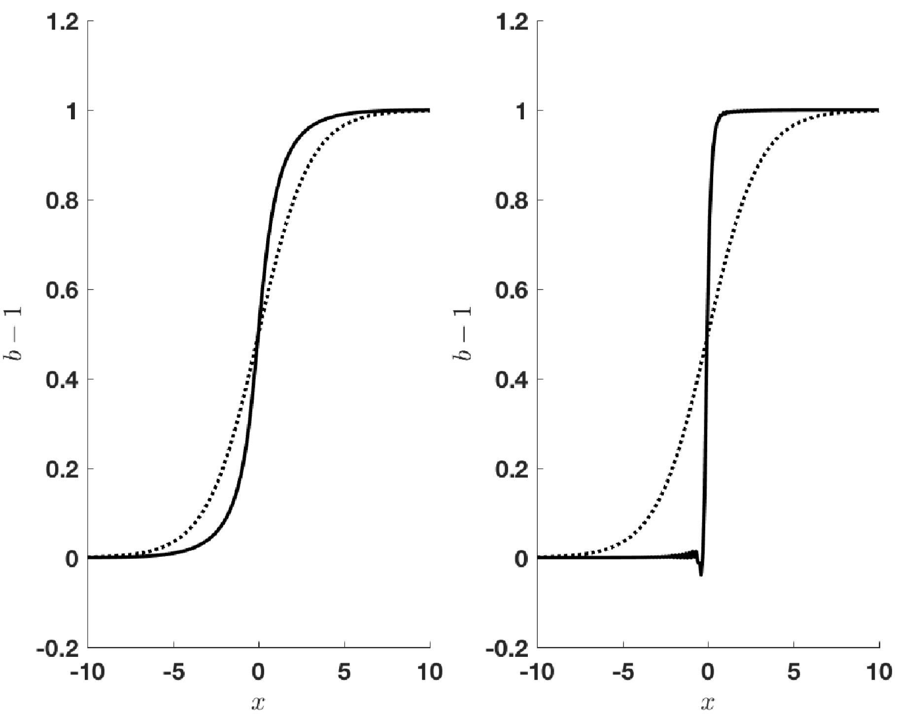
Initial (dotted line) and evolved profiles for
 $S=1$
.

Figure 1 shows two profiles achieved at two different times as a result of steepening for
 $S=1$
. The initial profile is shown by the dotted line. Although the dissipation and the dispersion terms are stiff, they appear to compete. In this case the dissipation is strong enough to ensure quick convergence to a final stationary state, which is not monotonic. This is clearly seen in movie 1 (online supplementary materials available at https://doi.org/10.1017/S0022377818000107). The steepening-un-steepening cycles are prevented by the strong dissipation and whistler wave trains are not generated. A phase-standing whistler is formed. Figure 2 shows two profiles for two different times for
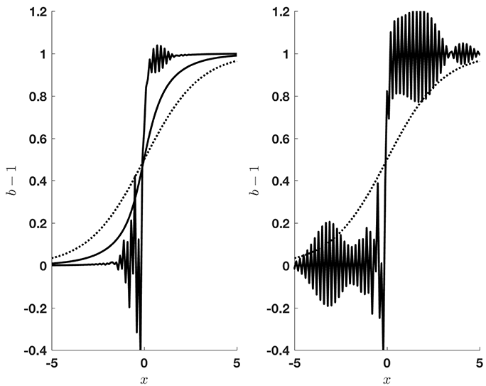
 $S=0.25$
. The ramp and the magnetic dip before the ramp are weakly time-dependent. Time-dependent wave trains in the form of enveloped short wavelength oscillations are generated both upstream and downstream by the steepened profile. The variations are illustrated in movie 2 (online supplementary materials). Finally, figure 3 shows two profiles achieved at two different times for
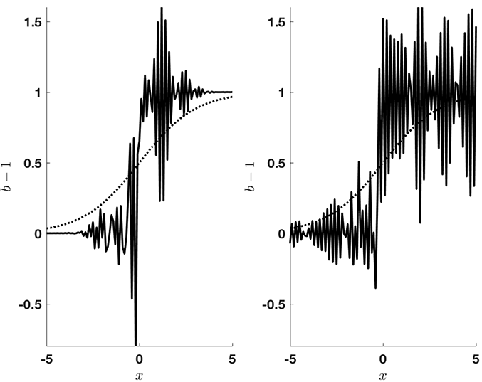
 $S=0.05$
. The two late profiles are quite different, which indicates essential non-stationarity of the shock front. The evolution of the profile in this case is shown in movie 3 (online supplementary materials). It is worth mentioning that although downstream wave trains are also present, they should not be taken seriously, since ion kinetics is important in this region and the assumptions of an isotropic polytropic state equation for ions are not valid in this region (Gedalin et al.
Reference Gedalin, Friedman and Balikhin2015a
). In low-Mach number, low-
 $\unicode[STIX]{x1D6FD}$
shocks the upstream plasma is not expected to be distorted substantially by the shock itself to break down the applied hydrodynamic approach. Yet, such distortions may occur and, if significant, would require a different treatment. In all cases, it is understood that the hydrodynamic approach is an approximation, and its validity for specific shock environment should be verified before applying the results obtained here.
Two profiles at two different times for
 $S=0.25$
and the initial profile (dotted line).

Two profiles at two different times for
 $S=0.005$
and the initial profile (dotted line).

7 Conclusions
We have shown that weak shocks with weak resistive dissipation can be described by KdV–Burgers equation. This equation is expected to possess stationary solutions. However, it is quite plausible that not any initial smooth profile with different asymptotical values of the magnetic field converges to the stationary point or that the convergence rate is extremely slow. In this case the profile will steepen until it begins to generate time-dependent wave trains which prevent further steepening. Thus, the shock profile is intrinsically time-dependent and stationary only on average. Although the wave trains are generated in a time-dependent manner, the time-dependence of the ramp (the main magnetic increase) may be weak for a range of dissipation parameters, so that the stationary approximation would be justified for the analysis of the ion motion across the shock front. If the dissipation is strong enough, the upstream wave train is also nearly stationary or even reduces to a small number of phase standing oscillations adjacent to the ramp. For sufficiently weak dissipation, propagating wave trains are formed with the changing shape and the shock front experiences reformation. These findings may explain the observed variety of the low-Mach number shock profiles (Farris et al.
Reference Farris, Russell and Thomsen1993; Wilson et al.
Reference Wilson, Cattell, Kellogg, Goetz, Kersten, Hanson, MacGregor and Kasper2007; Russell et al.
Reference Russell, Jian, Blanco-Cano and Luhmann2009; Kajdič et al.
Reference Kajdič, Blanco-Cano, Aguilar-Rodriguez, Russell, Jian and Luhmann2012; Wilson et al.
Reference Wilson III, Koval, Szabo, Stevens, Kasper, Cattell and Krasnoselskikh2017). Although a number of dissipation mechanisms have been proposed and the dissipation rate has been quantified (see Wilson et al.
Reference Wilson, Sibeck, Breneman, Contel, Cully, Turner, Angelopoulos and Malaspina2014, and references therein), translation of these findings into the corresponding dissipation parameter
 $\unicode[STIX]{x1D708}$
appearing in the two-fluid equations has yet to be done. Therefore, at this stage we are unable to present first-principle-based estimates for the control parameter
 $S$
. One of the possible scenarios of proceeding toward quantization of
 $S$
would be to include the dissipation produced by the wave-particle interaction with the participation of the generated whistlers themselves (Wilson et al.
Reference Wilson, Sibeck, Breneman, Contel, Cully, Turner, Angelopoulos and Malaspina2014; Oka et al.
Reference Oka, Wilson, Phan, Hull, Amano, Hoshino, Argall, Le Contel, Agapitov and Gershman2017).
Acknowledgement
This study was supported in part by the Israel Science Foundation (grant no. 368/14).
Supplementary movies
Supplementary movies are available at https://doi.org/10.1017/S0022377818000107.