1 Introduction
This work is on the free motion of a finite sized body in a wall-bounded shear flow. It is motivated by applications in external and internal flows.
If the body is an ice shard in a boundary layer of air flow on a wing the shard may impact locally upon the wing surface and freeze or cause damage or it may depart from the boundary layer and cause freezing or damage elsewhere on the vehicle, such as in an engine intake. This is important for heat transfer, for the aerodynamics of the wing and for safety reasons as well as flow transition (Gent et al. Reference Gent, Dart and Cansdale2000; Schmidt et al. Reference Schmidt, Young and Benard2010; Purvis & Smith Reference Purvis, Smith, Aston, Mulholland and Tate2016). In the case of other small bodies close to an airfoil or fuselage, such as debris or a parcel drop, the body may move towards the airfoil and even impact upon the airfoil surface. The occurrence again poses a potential hazard for both the surface and the body, in addition to the flow response. This form of fluid–body interaction raises questions of whether a detailed fluid-dynamical account can be given of the phenomenon and if so whether safety measures to avoid the phenomenon can be predicted. Similar questions arise in other external-flow interactions with bodies or particles such as dust and ice-shard motion (Einav & Lee Reference Einav and Lee1973; Wang & Levy Reference Wang and Levy2006) and internal-flow interactions such as those involved in plumbing problems, grain and rubble transport, dust movement in hoovers and transport of drugs or thrombi in blood vessel networks or lung airways (Portela et al. Reference Portela, Cota and Oliemans2002; Semwogerere & Weeks Reference Semwogerere and Weeks2008; Muller et al. Reference Muller, Fedosov and Gompper2014; Sinclair et al. Reference Sinclair, Lee, Schuster, Chiribi, Van Den Wijngaard, Van Horssen, Siebes, Spaan, Nagel and Smith2015).
The underlying flow throughout is one with zero slip at the wall(s). A point of issue is whether there is a preferred lateral direction for the body movement, in the sense that the body tends to migrate towards a nearby solid wall or away from it. Our particular interest lies in the mechanisms at increasing flow rates, especially concerned with the influences of different body shapes and parametric effects. When the fluid flow is at low Reynolds number a spherical body, circular cylinder in two dimensions, or a similarly shaped body, may be drawn gradually towards or away from a nearby wall: see Gavze & Shapiro (Reference Gavze and Shapiro1997), Frank et al. (Reference Frank, Anderson, Weeks and Morris2003), Kishori & Gu (Reference Kishori and Gu2010). With regard to the trend as inertia increases, various numerical simulations, experiments and empirical analyses have been performed at low or intermediate Reynolds numbers (Poesio et al. Reference Poesio, Ooms, Cate and Hunt2006; Loth & Dorgan Reference Loth and Dorgan2009; Kishori & Gu Reference Kishori and Gu2010) typically for spheres, circles or similar shapes. At medium-to-high Reynolds numbers slip streaming would suggest that in the presence of shear the lower velocity side of the body induces less pressure effect and so the overall pressure force should push the body into the lower velocity area of motion, thereby causing migration towards the wall. The present analytical approach suggests, in line with other approaches, that the above idea is incomplete and often incorrect because of significant unsteady responses in a full fluid–body interaction incorporating dependence on initial conditions and because of body-shape effects. Recent analytical studies by Smith & Ellis (Reference Smith and Ellis2010), Wilson & Smith (Reference Wilson and Smith2013), Smith & Johnson (Reference Smith and Johnson2016) for settings quite different from the present one likewise suggest shape dependence. They also indicate considerable initial value dependence.
Major examples where the fluid and body motions affect each other substantially in near-wall shear flow are the boundary layer (Hall Reference Hall1964; Einav & Lee Reference Einav and Lee1973; Petrie et al. Reference Petrie, Morris, Bajwa and Vincent1993; Wang & Levy Reference Wang and Levy2006; Schmidt & Young Reference Schmidt and Young2009; Schmidt et al. Reference Schmidt, Young and Benard2010) and channel flow (Portela et al. Reference Portela, Cota and Oliemans2002; Smith & Ellis Reference Smith and Ellis2010; Loisel et al. Reference Loisel, Abbas, Masbernat and Climen2013; Smith & Johnson Reference Smith and Johnson2016), whether for a single body or many bodies. Increased physical understanding of the detailed interaction between fluid flow and a single finite body contained within it may lead to improved models for many-particle interactions involving particles of finite sizes (Schmidt et al. Reference Schmidt, Young and Benard2010; Smith & Johnson Reference Smith and Johnson2016). This is supplementary to bulk modelling of multi particle phenomena. The body of interest here is short compared with the boundary-layer development length, which is typically an airfoil chord, and the body is located laterally in the middle of the oncoming boundary layer under a given free-stream velocity. The body is relatively thin but of length large compared with the boundary-layer thickness (or large compared with the vessel width in the case of channel flow).
The work is partially complementary to the recent study of Smith & Johnson (Reference Smith and Johnson2016) on shorter bodies in channel flow. Their study indicates various time scales of concern and identifies an unusual instability. We take this up by addressing steady flow first in a boundary layer and unsteadiness later, followed by consideration of possible stabilising effects. The present work also differs from the study above because the present focus is on rather longer length scales and the work covers boundary layers as well as channels. The emphasis is on high Reynolds numbers and analytical features to be complementary to numerical simulations and experiments. Viscous–inviscid interplay involving significant contributions from an inviscid core response and viscous sublayers has a decisive role in the fluid–body interactions of interest here.
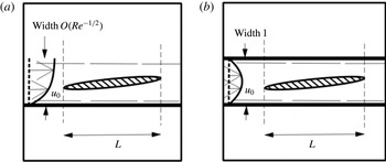
The body of length
 $L$
in
 $(a)$
a laminar boundary layer of width
 $O(Re^{-1/2})$
with dashed lines indicating the induced viscous wall layer and the effective edge of the boundary layer,
 $(b)$
a channel flow of width unity where dashes indicate the two viscous wall layers. Sketch not to scale.

The fluid is incompressible and its motion is assumed to be two-dimensional and laminar. Section 2 considers the behaviour induced within a boundary layer (see figure 1 a) by the presence of a finite rigid body fixed in the midst of the layer, allowing for multi-scale structure as well as distinct leading edge and trailing edge conditions. Solution properties presented in § 3 include the wall pressure and skin friction or wall shear stress. Section 4 then describes the analogous problem in a channel (see figure 1 b) and shows the same reduced problem and detailed solution properties apply there. Unsteady behaviour is accommodated in § 5 with the body moving freely in response to the flow pressure forces according to Newton’s second law and thus changing the flow field and vice versa. This full fluid–body interaction can result in instability. Stabilisation is achievable however as described in § 6, while final comments are given in § 7. Three specific stabilising factors are explored in detail.
2 Flow response in the boundary layer
The length scales involved are considerably less than the development length of the boundary layer and so the surrounding boundary-layer flow is almost unidirectional. A non-dimensionalisation is made in which fluid-flow velocities are measured relative to the free-stream velocity
 $u^{\ast }$
at the edge of the boundary layer, lengths are measured with respect to the development length
 $a^{\ast }$
, which is typically the airfoil chord in aerodynamics and the Reynolds number
 $Re$
(
 $\gg 1$
) is
 $u^{\ast }a^{\ast }/\unicode[STIX]{x1D708}^{\ast }$
where
 $\unicode[STIX]{x1D708}^{\ast }$
is the kinematic viscosity of the fluid. A single asterisk denotes a dimensional quantity. The pressure is based on
 $\unicode[STIX]{x1D70C}^{\ast }{u^{\ast }}^{2}$
, with
 $\unicode[STIX]{x1D70C}^{\ast }$
being the fluid density. In non-dimensional terms the boundary layer occupies
 $y>0$
and has width
 $O(Re^{-1/2})$
and length
 $O(1)$
whereas the body length
 $L\ll 1$
; the planar Cartesian coordinates are
 $x$
,
 $y$
, respectively horizontal and vertical as in figure 1(a), the corresponding flow velocity components are
 $u$
,
 $v$
and the pressure is
 $p$
relative to the free-stream value which is taken as zero. The characteristic streamwise flow velocity is of order unity.
The body which is currently considered as fixed, or moving with negligible velocity, is closed, is of uniform density and may be of thickness comparable with the boundary-layer thickness whereas its underside is approximately parallel with the wall on the boundary-layer scale. Far upstream of the thin body the incident flow is almost unidirectional with profiles
 $u_{0}(\bar{y})$
,
 $Re^{-1/2}\unicode[STIX]{x1D713}_{0}(\bar{y})$
for the velocity
 $u$
and streamfunction
 $\unicode[STIX]{x1D713}$
where
 $u_{0}(\bar{y})=\unicode[STIX]{x1D713}_{0}^{\prime }(\bar{y})$
and
 $y=Re^{-1/2}\bar{y}$
. The prime denotes a
 $\bar{y}$
derivative. The profiles are of general
 $O(1)$
form with a positive velocity except at the wall
 $\bar{y}=0$
, with a normalised skin friction
 $u_{0}^{\prime }(0)=Re^{1/2}\unicode[STIX]{x1D706}$
at that wall and with uniform flow say
 $u_{0}=1$
at large
 $\bar{y}$
. Orders of magnitude as in Stewartson (Reference Stewartson1970), Sychev (Reference Sychev1972), Smith (Reference Smith1973), Smith & Daniels (Reference Smith and Daniels1981), Smith & Ellis (Reference Smith and Ellis2010) then indicate that the flow structure comprises a core of two quasi-inviscid parts, one above and the other below the body, a viscous wall layer near
 $\bar{y}=0$
and two viscous layers on the body itself, in addition to which at least one adjustment zone is induced near the leading edge of the body.
The underside of the body, nearly aligned with the wall as in figure 1(a), lies at a scaled height
 $\bar{y}=\bar{y}_{0}$
(
 $=O(1)$
) inside the boundary layer. The streamwise length scale
 $L$
of the body is such that within the majority of the surrounding fluid motion there is insignificant normal variation in the pressure except across the body itself and the viscous wall layer remains thin compared with the boundary-layer width. The insignificance of the normal pressure gradient implies that
 $L$
is greater than
 $O(Re^{-3/8})$
and no significant upstream influence occurs over the scale of
 $L$
(Smith Reference Smith1973; White & Smith Reference White and Smith2012), while the wall layer property agrees with
 $L$
being less than
 $O(1)$
. Next we present details in § 2.1 for readers more interested in the detailed scales, fluid-dynamical structure and interactions, as well as the application to channel flow in a later section, followed in § 2.2 by the summarised problem which leads on to solution properties in other subsequent sections.
2.1 Details of the fluid–body interplay
The wall layer has thickness
 $O(L^{1/3}Re^{-1/2})$
from an inertial–viscous balance of momentum and so the major part (the core) of the flow where
 $\bar{y}$
is
 $O(1)$
is expected to be inviscid. This indicates the orders of magnitude of the disturbance in the core if significant interaction is to take place. Thus
 $$\begin{eqnarray}\displaystyle x=LX\quad \text{with }Re^{-3/8}\ll L\ll 1, & & \displaystyle\end{eqnarray}$$
and the flow solution is expanded in the following form, where
 $\unicode[STIX]{x1D716}$
denotes an arbitrary small amplitude parameter representing the relative displacement due to the underside of the body,
 $$\begin{eqnarray}\displaystyle [u,\unicode[STIX]{x1D713},p]=\left[u_{0},Re^{-1/2}\unicode[STIX]{x1D713}_{0},0\right]+\unicode[STIX]{x1D716}\left[L^{1/3}u_{1},L^{1/3}Re^{-1/2}\unicode[STIX]{x1D713}_{1},L^{2/3}p_{1}\right]+\cdots \,. & & \displaystyle\end{eqnarray}$$
This is for
 $\bar{y}$
of
 $O(1)$
in both parts of the core below and above the thin body in the figure. The unknown perturbations
 $u_{1}$
,
 $\unicode[STIX]{x1D713}_{1}$
,
 $p_{1}$
are functions of
 $X$
,
 $\bar{y}$
to be found, subject to the perturbations having to tend to zero upstream to match with the incident flow properties. Substitution into the Navier–Stokes equations then yields to leading order
 $u_{1}=\unicode[STIX]{x2202}\unicode[STIX]{x1D713}_{1}/\unicode[STIX]{x2202}\bar{y}$
,
 $v_{1}=-\unicode[STIX]{x2202}\unicode[STIX]{x1D713}_{1}/\unicode[STIX]{x2202}X$
,
 $u_{0}\unicode[STIX]{x2202}u_{1}/\unicode[STIX]{x2202}X+v_{1}u_{0}^{\prime }=0$
and
 $\unicode[STIX]{x2202}p_{1}/\unicode[STIX]{x2202}\bar{y}=0$
in the continuity and
 $x$
-,
 $y$
-momentum equations. Hence a simple displacement effect holds in each part of the core,
 $$\begin{eqnarray}\displaystyle u_{1}=A^{\pm }(X)u_{0}^{\prime }(\bar{y}),\quad \unicode[STIX]{x1D713}_{1}=A^{\pm }(X)u_{0}(\bar{y}),\quad p_{1}=P^{\pm }(X), & & \displaystyle\end{eqnarray}$$
with the pressures
 $P^{\pm }$
and effective negative displacements
 $A^{\pm }$
being unknown and the superscripts
 $\pm$
referring to the core flows above and below the body respectively.
The underside thickness of the body occupying
 $0\leqslant X\leqslant 1$
is assumed slightly less than that of the viscous wall layer, on account of the small factor
 $\unicode[STIX]{x1D716}$
, and for clarity the same size is taken for the topside (although this will be extended below). The non-zero velocity
 $u_{0}$
at height
 $Re^{-1/2}\bar{y}_{0}$
implies that the zero-normal-flow condition must apply on the body surfaces
 $$\begin{eqnarray}\displaystyle y=Re^{-1/2}\bar{y}_{0}+\unicode[STIX]{x1D716}L^{1/3}Re^{-1/2}f^{\pm }(X)\quad \text{for }0<X<1, & & \displaystyle\end{eqnarray}$$
say. The fluid flow is separation free and the Blasius-like viscous layers on the upper and lower body surfaces remain negligibly thin as in Smith & Jones (Reference Smith and Jones2000). The kinematic boundary condition becomes
 $$\begin{eqnarray}\displaystyle A^{\pm }=-f^{\pm }+K^{\pm }\quad \text{for }0<X<1, & & \displaystyle\end{eqnarray}$$
where
 $K^{\pm }$
are unknown constants. This is because the condition requires
 $\unicode[STIX]{x1D713}$
to be constant on the surfaces (2.4) and so by expansion
 $\unicode[STIX]{x1D713}_{0}(\bar{y}_{0}^{\pm })+\unicode[STIX]{x1D716}L^{1/3}f^{\pm }\unicode[STIX]{x1D713}_{0}^{\prime }(\bar{y}_{0}^{\pm })+\cdots +\unicode[STIX]{x1D716}L^{1/3}\unicode[STIX]{x1D713}_{1}^{\prime }(\bar{y}_{0}^{\pm })+\cdots \,$
is constant. Hence at order
 $\unicode[STIX]{x1D716}L^{1/3}$
we have
 $f^{\pm }u_{0}(\bar{y}_{0}^{\pm })+A^{\pm }u_{0}(\bar{y}_{0}^{\pm })$
being constant, from which (2.5) is obtained.
The flow field on top of the body extends to the outer parts of the boundary layer where free-stream properties hold. Hence in particular
 $$\begin{eqnarray}\displaystyle P^{+}=0\quad \text{for }0<X<1. & & \displaystyle\end{eqnarray}$$
The condition (2.6) applies over the present length scales even when the topside of the body is more extensive, for example of thickness comparable with the boundary-layer thickness. By contrast the flow underneath induces a non-zero pressure response
 $P^{-}$
by means of viscous effects. The viscous wall layer near
 $y=0$
is described by
 $y=L^{1/3}Re^{-1/2}Y$
and the expansion (Smith & Jones Reference Smith and Jones2000)
 $$\begin{eqnarray}\displaystyle [u,\unicode[STIX]{x1D713},p]=\left[L^{1/3}\unicode[STIX]{x1D706}Y,{\textstyle \frac{1}{2}}L^{2/3}Re^{-1/2}\unicode[STIX]{x1D706}Y^{2},0\right]+\unicode[STIX]{x1D716}\left[L^{1/3}U,L^{2/3}Re^{-1/2}\unicode[STIX]{x1D6F9},L^{2/3}P\right]+\cdots \,, & & \displaystyle\end{eqnarray}$$
where
 $P=P^{-}$
by virtue of the normal momentum equation. Hence the governing equations are those of a viscous–inviscid wall layer,
 $$\begin{eqnarray}\displaystyle & \displaystyle U=\unicode[STIX]{x1D6F9}_{Y}, & \displaystyle\end{eqnarray}$$
 $$\begin{eqnarray}\displaystyle & \displaystyle V=-\unicode[STIX]{x1D6F9}_{X}, & \displaystyle\end{eqnarray}$$
 $$\begin{eqnarray}\displaystyle & \displaystyle \unicode[STIX]{x1D706}YU_{X}+V\unicode[STIX]{x1D706}=-P_{X}^{-}+U_{YY}, & \displaystyle\end{eqnarray}$$
subject to the requirements
 $$\begin{eqnarray}\displaystyle & \displaystyle U=0\quad \text{at }Y=0, & \displaystyle\end{eqnarray}$$
 $$\begin{eqnarray}\displaystyle & \displaystyle V=0\quad \text{at }Y=0, & \displaystyle\end{eqnarray}$$
 $$\begin{eqnarray}\displaystyle & \displaystyle U\rightarrow \unicode[STIX]{x1D706}A^{-}(X)\quad \text{as }Y\rightarrow \infty . & \displaystyle\end{eqnarray}$$
These are for no slip at the wall and for matching with the core solution respectively. The unknown pressure and displacement here yield viscous–inviscid interaction. The overall system is of elliptic type due to the requirements on the
 $P^{-}$
,
 $A^{-}$
solution and specifically the property that
 $$\begin{eqnarray}\displaystyle P^{+}=P^{-}=0\quad \text{for }0<X,X>1\quad \text{and}\quad A^{-}=0\quad \text{for }X<0. & & \displaystyle\end{eqnarray}$$
This arises because of the classical boundary layer in
 $X<0$
,
 $X>1$
, the body being absent there. No pressure response occurs at such
 $X$
values and there is a displacement effect only:
 $A^{+}=A^{-}$
is generally non-zero in the wake
 $X>1$
and this scaled wake displacement is to be determined (in contrast with the result
 $A^{+}=A^{-}=0$
upstream). In addition as stated earlier no significant normal pressure gradient acts over the current streamwise scale.
An Euler-like zone and a viscous–inviscid zone are produced near the leading edge (Smith & Ellis Reference Smith and Ellis2010; Smith & Johnson Reference Smith and Johnson2016). The zones which are shorter horizontally than the long scale in (2.1) are necessary to account for the slight change across
 $X=0\pm$
in streamline height due to the unknown values
 $K^{\pm }$
on the body by virtue of (2.2)–(2.5) as well as abrupt changes in derivatives of velocity and pressure locally. The smooth adjustment locally is achieved by a combination of predominantly inviscid behaviour over an axial scale of order
 $Re^{-1/2}$
near the leading edge and viscous–inviscid interplay over the axial scale of order
 $Re^{-3/8}$
(compare with (2.1)), both of which admit upstream influence ahead of the body itself. The
 $Re^{-3/8}$
scale ensures continuity of displacement by means of an
 $Re^{3/8}x$
functional dependence and the corresponding pressure variation is small relative to that in (2.2) while the
 $O(Re^{-1/2})$
scale then allows for the slope of the displacement to be made continuous. Further, the leading edge behaviour here has to accommodate the feature that the streamfunction
 $\unicode[STIX]{x1D713}$
must be continuous on the body, hence
 $A^{\pm }u_{0}(\bar{y})$
must be continuous everywhere on the body from (2.3), hence
 $A^{\pm }$
must be continuous at
 $X=0+$
and hence
 $K^{\pm }$
are equal from (2.5) since the upper and lower body surface shapes
 $f^{\pm }$
are identical at
 $X=0$
. This leads to the relation
 $$\begin{eqnarray}\displaystyle K^{+}=K^{-}=K, & & \displaystyle\end{eqnarray}$$
say. At the trailing edge
 $X=1$
a Kutta-like condition applies in order to keep the flow separation free and continuity of pressure holds across the wake (Smith & Ellis Reference Smith and Ellis2010; Smith & Johnson Reference Smith and Johnson2016), requiring
 $$\begin{eqnarray}\displaystyle P^{-}=0\quad \text{at }X=1, & & \displaystyle\end{eqnarray}$$
by virtue of (2.14). The quasi-height
 $K$
in (2.15) based on the streamfunction acts as a circulation constant and has to adjust or be adjusted to ensure that (2.16) is satisfied, a condition which highlights the spatial ellipticity.
2.2 Summarised problem
The task in summary is that of solving viscous equations and interactive conditions, in the following neater form:
 $$\begin{eqnarray}\displaystyle & \displaystyle U=\unicode[STIX]{x1D6F9}_{Y},\quad V=-\unicode[STIX]{x1D6F9}_{X}, & \displaystyle\end{eqnarray}$$
 $$\begin{eqnarray}\displaystyle & \displaystyle \unicode[STIX]{x1D706}YU_{X}+V\unicode[STIX]{x1D706}=-P_{X}+U_{YY}, & \displaystyle\end{eqnarray}$$
 $$\begin{eqnarray}\displaystyle & \displaystyle U=V=0\quad \text{at }Y=0, & \displaystyle\end{eqnarray}$$
 $$\begin{eqnarray}\displaystyle & \displaystyle U\rightarrow \unicode[STIX]{x1D706}\{K-f_{u}(X)-h-(X-{\textstyle \frac{1}{2}})\unicode[STIX]{x1D703}\}\quad \text{as }Y\rightarrow \infty , & \displaystyle\end{eqnarray}$$
 $$\begin{eqnarray}\displaystyle & \displaystyle P(0)=P(1)=0, & \displaystyle\end{eqnarray}$$
for
 $U$
,
 $V$
,
 $P$
,
 $K$
. This flow problem is almost one of the viscous–inviscid kind with fixed displacement and unknown pressure as studied in previous works (Smith & Daniels Reference Smith and Daniels1981; White & Smith Reference White and Smith2012; Pruessner & Smith Reference Pruessner and Smith2015) but here the circulation constant
 $K$
is also unknown and that ties in with the presence of a downstream requirement at
 $X=1$
in (2.21). Here
 $f_{u}(X)$
is the prescribed shape of the underbody. The contributions
 $h$
,
 $\unicode[STIX]{x1D703}$
are due to changes in the lateral location and orientation of the body, scaled on
 $\unicode[STIX]{x1D716}L^{1/3}Re^{-1/2}$
and
 $\unicode[STIX]{x1D716}L^{-2/3}Re^{-1/2}$
respectively, and these are also taken as prescribed at this stage.
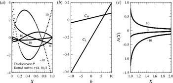
 $(a)$
Scaled pressure
 $P$
(thick curves) and skin-friction perturbation
 $\unicode[STIX]{x1D70F}/\unicode[STIX]{x1D6FF}$
(dotted curves) at the wall, versus scaled distance
 $X$
, for parabolic undershape (3.1) when
 $h=\unicode[STIX]{x1D703}=1$
. Values of the thickness parameter
 $b$
are indicated.
 $(b)$
Lift
 $C_{L}$
and torque or moment
 $C_{M}$
versus
 $b$
; both change sign as
 $b$
increases.
 $(c)$
Wake displacement
 $A$
versus
 $X$
(
 ${>}1$
) for
 $b$
values of
 $-10,0,10$
.

3 Solution properties in the boundary layer
The detailed solving and results for a general body shape are given in appendix A.
For the specific example of a parabolic-shaped underbody, namely
 $$\begin{eqnarray}\displaystyle f_{u}(X)=bX(1-X)\quad \text{for }0<X<1, & & \displaystyle\end{eqnarray}$$
with
 $b$
being a positive or negative constant corresponding to the underbody curvature, the above results give the explicit responses
 $$\begin{eqnarray}\displaystyle P=\unicode[STIX]{x1D6FE}\left\{3X^{1/3}(h-K)+\left({\textstyle \frac{9}{4}}X^{4/3}-{\textstyle \frac{3}{2}}X^{1/3}\right)\unicode[STIX]{x1D703}+{\textstyle \frac{9}{28}}b\left(7X^{4/3}-6X^{7/3}\right)\right\}, & & \displaystyle\end{eqnarray}$$
with
 $$\begin{eqnarray}\displaystyle K=h+\frac{\unicode[STIX]{x1D703}}{4}+\frac{3b}{28}, & & \displaystyle\end{eqnarray}$$
while the perturbation in skin friction has the explicit form, with
 $$\begin{eqnarray}\displaystyle \unicode[STIX]{x1D6FF}=3A_{i}(0)\unicode[STIX]{x1D706}^{4/3}/\unicode[STIX]{x1D6E4}\left({\textstyle \frac{2}{3}}\right) & & \displaystyle\end{eqnarray}$$
being a positive constant,
 $$\begin{eqnarray}\displaystyle \unicode[STIX]{x1D70F}(X,0)=\unicode[STIX]{x1D6FF}\left\{3X^{-1/3}\left(K-h+{\textstyle \frac{1}{2}}\unicode[STIX]{x1D703}\right)-{\textstyle \frac{3}{2}}(\unicode[STIX]{x1D703}+b)X^{2/3}+{\textstyle \frac{9}{5}}bX^{5/3}\right\}. & & \displaystyle\end{eqnarray}$$
The solutions for the scaled wall pressure and the skin-friction perturbation are presented in figure 2(a) for a range of values of the upwards curvature or thickness parameter
 $b$
, with
 $h$
,
 $\unicode[STIX]{x1D703}$
taken as unity as a typical example. It is observed that only the combination
 $h_{K}=h-K$
affects the flow solutions. Increasing the upwards curvature parameter
 $b$
raises the pressures near the rear of the body and lowers those near the front as may be anticipated physically. The skin-friction response near the leading edge is singular and this is due overwhelmingly to the jump in the effective displacement A whereas near the trailing edge the skin friction reacts to the favourable pressure gradient for
 $b$
of
 $10$
by increasing and to the adverse value for
 $b$
of
 $-10$
by decreasing as expected.
Also shown in figure 2(b) is the scaled lift
 $C_{L}$
and torque or moment
 $C_{M}$
acting on the body. Since the pressure produced on the topside of the body is much less than that beneath the body (in view of (2.6)) the lift and torque are dominated by the influence of the underneath pressure solution: see appendix A. The effects from viscous stresses are substantially smaller. Hence the scaled lift and torque are given by
 $$\begin{eqnarray}\displaystyle & \displaystyle C_{L}=\int _{0}^{1}P(X)\,\text{d}X, & \displaystyle\end{eqnarray}$$
 $$\begin{eqnarray}\displaystyle & \displaystyle C_{M}=\int _{0}^{1}\left(X-\frac{1}{2}\right)P(X)\,\text{d}X, & \displaystyle\end{eqnarray}$$
under the assumption that the centre of mass lies at the central position
 $X=1/2$
. In the case of the underbody shape (3.1) the lift and torque results are
 $$\begin{eqnarray}\displaystyle & \displaystyle C_{L}=9\unicode[STIX]{x1D6FE}\left\{\frac{h_{K}}{4}-\frac{\unicode[STIX]{x1D703}}{56}+\frac{3b}{70}\right\}, & \displaystyle\end{eqnarray}$$
 $$\begin{eqnarray}\displaystyle & \displaystyle C_{M}=9\unicode[STIX]{x1D6FE}\left\{\frac{h_{K}}{56}+\frac{\unicode[STIX]{x1D703}}{80}+\frac{3b}{728}\right\}. & \displaystyle\end{eqnarray}$$
The dependence on the curvature parameter
 $b$
in the figure is of interest. The changes in sign for both
 $C_{L}$
,
 $C_{M}$
arise directly because of the pressure behaviour in figure 2(a). Increasing
 $b$
implies that the underbody shape becomes more concave downwards such that lift and torque are enhanced.
Downstream of the body in
 $X>1$
a wake occurs in which (2.14) applies to the emergent displacements and pressures. Clearly the pressures are zero. Application of the general results in appendix A to the displacement problem then gives
 $$\begin{eqnarray}\displaystyle A(X)=\unicode[STIX]{x1D6FF}_{2}\unicode[STIX]{x1D706}^{-5/3}\int _{0}^{1}P(S)(X-S)^{-4/3}\,\text{d}S,\quad \text{for }X>1, & & \displaystyle\end{eqnarray}$$
allowing
 $A(=A\pm )$
in the wake to be determined from the pressures acting on the body. The constant
 $\unicode[STIX]{x1D6FF}_{2}=-1/(9A_{i}^{\prime }(0)\unicode[STIX]{x1D6E4}(2/3))$
(approximately equal to
 $0.31703$
) is positive. The condition (2.16) ensures convergence of the integral in (3.10). Results are shown in figure 2(c) with
 $h$
,
 $\unicode[STIX]{x1D703}$
again unity for the parabolic undershape and tend to confirm the algebraic
 $X^{-4/3}$
decay at large positive
 $X$
seen in (3.10) with the coefficient of proportionality being related to the scaled lift on the body. The displacement in the wake is continuous with that from the given body shape at the trailing edge: for example a zero b value in (3.10) gives an
 $A$
value of
 $-0.25$
immediately downstream of the trailing edge which agrees with the result
 $-\unicode[STIX]{x1D703}/4$
from the underbody effect at the trailing edge.
4 Solution properties in channel flow
A similar physical reasoning is found to apply for a thin body in channel flow over length scales suitably larger than the channel width
 $a^{\ast }$
. With a Reynolds number
 $R$
based conventionally on this
 $a^{\ast }$
(instead of the development length used in
 $Re$
) and on the typical axial incident velocity, the coordinates
 $x$
,
 $y$
are as in figure 1(b) and the channel walls are at
 $y=0$
,
 $1$
. The incident profiles
 $u_{0}(y)$
,
 $\unicode[STIX]{x1D713}_{0}(y)$
yield positive velocity except at
 $y=0$
,
 $1$
, with a normalised wall shear stress
 $u_{0}^{\prime }(0)=\unicode[STIX]{x1D706}^{-}$
of order unity at the lower wall and similarly at the upper wall
 $u_{0}^{\prime }(1)=-\unicode[STIX]{x1D706}^{+}$
say. Here
 $R$
is large and the orders of magnitude of the main properties then are as in Smith (Reference Smith1976, Reference Smith1977).
The core flow has
 $x=LX$
with
 $R^{1/7}\ll L\ll R$
and a simple displacement takes place in each part of the core,
 $$\begin{eqnarray}\displaystyle & & \displaystyle \hspace{-8.99994pt}[u,\unicode[STIX]{x1D713},p]=\left[u_{0},\unicode[STIX]{x1D713}_{0},0\right]\nonumber\\ \displaystyle & & \displaystyle \hspace{-8.99994pt}\quad +\,\unicode[STIX]{x1D716}\left[L^{1/3}R^{-1/3}A^{\pm }(X,T)u_{0}^{\prime }(y),L^{1/3}R^{-1/3}A^{\pm }(X,T)u_{0}(y),L^{2/3}R^{-2/3}P^{\pm }(X)\right]+\cdots \,.\qquad \quad\end{eqnarray}$$
The body surfaces are prescribed as
 $y=y_{0}+\unicode[STIX]{x1D716}L^{1/3}R^{-1/3}f^{\pm }(X)$
for
 $0<X<1$
and so the upper and lower displacement effects are given by
 $$\begin{eqnarray}\displaystyle A^{\pm }=-f^{\pm }+K^{\pm },\quad 0<X<1, & & \displaystyle\end{eqnarray}$$
respectively. The lower viscous wall layer near
 $y=0$
is described by
 $y=L^{1/3}R^{-1/3}Y$
and the expansion (Smith Reference Smith1976)
 $$\begin{eqnarray}\displaystyle [u,\unicode[STIX]{x1D713},p] & = & \displaystyle \left[L^{1/3}R^{-1/3}\unicode[STIX]{x1D706}^{-}Y,{\textstyle \frac{1}{2}}L^{2/3}R^{-2/3}\unicode[STIX]{x1D706}^{-}Y^{2},0\right]\nonumber\\ \displaystyle & & \displaystyle +\,\unicode[STIX]{x1D716}[L^{1/3}R^{-1/3}U^{-},L^{2/3}R^{-2/3}\unicode[STIX]{x1D6F9}^{-},L^{2/3}R^{-2/3}P^{-}]+\cdots \,,\end{eqnarray}$$
with an analogous form holding in the upper viscous wall layer. Hence the governing equations and boundary conditions are
 $$\begin{eqnarray}\displaystyle & \displaystyle U^{\pm }=\unicode[STIX]{x1D6F9}_{Y}^{\pm },\quad V^{\pm }=-\unicode[STIX]{x1D6F9}_{X}^{\pm }, & \displaystyle\end{eqnarray}$$
 $$\begin{eqnarray}\displaystyle & \displaystyle \unicode[STIX]{x1D706}^{\pm }YU_{X}^{\pm }+V^{\pm }\unicode[STIX]{x1D706}^{\pm }=-P_{X}^{\pm }+U_{YY}^{\pm }, & \displaystyle\end{eqnarray}$$
 $$\begin{eqnarray}\displaystyle & \displaystyle U^{\pm }=V^{\pm }=0\quad \text{at }Y=0, & \displaystyle\end{eqnarray}$$
 $$\begin{eqnarray}\displaystyle & \displaystyle U^{\pm }\rightarrow \mp \unicode[STIX]{x1D706}^{\pm }A^{\pm }(X)\quad \text{as }Y\rightarrow \infty , & \displaystyle\end{eqnarray}$$
in the two wall layers. Also the arguments behind (2.15), (2.16) apply still, slightly modified and yielding
 $K^{+}=K^{-}=K$
,
 $P^{+}=P^{-}$
at
 $X=1$
, while the upstream and downstream relations give
 $$\begin{eqnarray}\displaystyle A^{+}=A^{-},P^{+}=P^{-},\quad \text{for }X<0\quad \text{and }X>1, & & \displaystyle\end{eqnarray}$$
since the body is absent there and no significant normal pressure gradient acts there. An axial length scale of order
 $R^{1/7}$
(
 $\ll L$
) acts to provide continuity of displacement upstream through an
 $\exp (\bar{\unicode[STIX]{x1D705}}R^{-1/7}x)$
process where
 $\bar{\unicode[STIX]{x1D705}}$
is a positive constant (Smith Reference Smith1977).
The same final problem as in § 2.2 is found to apply here but for reasons slightly different from those for the boundary layer. If the incident wall shears
 $\unicode[STIX]{x1D706}^{\pm }$
in the channel flow are equal then subtraction of the upper and lower wall-layer systems above leads to (2.17)–(2.21) precisely but with
 $$\begin{eqnarray}\left[U^{+}-U^{-},V^{+}-V^{-},P^{+}-P^{-},{\textstyle \frac{1}{2}}(A^{+}+A^{-})\right]=\left[U,V,P,K-f_{u}-h-(X-{\textstyle \frac{1}{2}})\unicode[STIX]{x1D703}\right]\end{eqnarray}$$
representing the differences between the upper and lower wall pressures and the means of the displacements. The central problem (2.17)–(2.21) has the same form as those studied by Smith & Jones (Reference Smith and Jones2000), White & Smith (Reference White and Smith2012) for symmetric channel flow over shorter length scales, except that in their studies the
 $K$
contribution is absent because of symmetry across the channel and no downstream condition analogous to (2.21) is involved. The pressure differences and mean displacements in the present setting are seen to act similarly to the pressure and displacement effects in the boundary-layer case. The flow properties in channel flow are thus exactly as described in the previous section.
5 Unsteady flow–body interaction
When the rigid body is free to move the scaled lift and torque in (3.6) and (3.7) act along with gravity to drive the changes in linear and angular momentum of the body by means of Newton’s second law. This is considered below mainly with the boundary-layer case in mind but it applies equally well for the channel-flow case as well.
The scaled height
 $h$
and angle
 $\unicode[STIX]{x1D703}$
thus become time dependent. In dimensional orders of magnitude the lateral linear momentum terms are
 $O(M^{\ast }u^{\ast }Re^{-1/2}\unicode[STIX]{x1D716}L^{1/3}\unicode[STIX]{x1D70E}^{-1})$
where
 $M^{\ast }$
is the body mass and the time scale is written
 $a^{\ast }{u^{\ast }}^{-1}\unicode[STIX]{x1D70E}$
. So the rate of change of linear momentum is
 $O(M^{\ast }{u^{\ast }}^{2}{a^{\ast }}^{-1}Re^{-1/2}\unicode[STIX]{x1D716}L^{1/3}\unicode[STIX]{x1D70E}^{-2})$
in the lateral direction. The forces to balance the rate of change are dominated by the
 $C_{L}$
influence in (3.6) which gives a lift force of
 $O(\unicode[STIX]{x1D70C}^{\ast }{u^{\ast }}^{2}a^{\ast })$
accompanied by a gravity force which we take to be comparable. Hence the time scale satisfies
 $\unicode[STIX]{x1D70E}^{2}\sim M^{\ast }{a^{\ast }}^{-2}{\unicode[STIX]{x1D70C}^{\ast }}^{-1}Re^{-1/2}\unicode[STIX]{x1D716}L^{1/3}$
. Similar reasoning applies to the angular momentum. On the other hand the streamwise component of the linear momentum balance for the body simply gives
 $\text{d}^{2}X_{c}/dX^{2}$
as zero predominantly where
 $X=X_{c}$
is the streamwise position of the centre of mass; the streamwise forces due to the fluid motion (pressure and stress forces) are too small to affect the main response which is that
 $X_{c}$
may move with a constant velocity
 $V_{c}$
. We take
 $V_{c}$
to be negligible in the present and the preceding settings but explore the influence of non-negligible
 $V_{c}$
in the next section.
The height and the orientation angle vary in time according to the balances of lateral momentum and angular momentum,
 $$\begin{eqnarray}\displaystyle & \displaystyle \hat{M}\frac{\text{d}^{2}h}{\text{d}T^{2}}=C_{L}-\hat{M}{\hat{g}}, & \displaystyle\end{eqnarray}$$
 $$\begin{eqnarray}\displaystyle & \displaystyle \hat{I} \frac{\text{d}^{2}\unicode[STIX]{x1D703}}{\text{d}T^{2}}=C_{M}, & \displaystyle\end{eqnarray}$$
which hold at leading order. Here
 $\hat{M}$
,
 $\hat{I}$
are defined by
 $L^{-4/3}Re^{1/3}M^{\ast }/({a^{\ast }}^{2}\unicode[STIX]{x1D70C}^{\ast }\unicode[STIX]{x1D70E}^{2})$
and
 $L^{-7/3}Re^{1/3}I^{\ast }/({a^{\ast }}^{4}\unicode[STIX]{x1D70C}^{\ast }\unicode[STIX]{x1D70E}^{2})$
where the dimensional mass
 $M^{\ast }$
and moment of inertia
 $I^{\ast }$
of the body per unit distance perpendicular to the plane of the motion are themselves comparable with or greater than
 $L^{1/3}Re^{-1/3}{a^{\ast }}^{2}\unicode[STIX]{x1D70C}_{B}^{\ast }$
,
 $L^{1/3}Re^{-1/3}{a^{\ast }}^{4}\unicode[STIX]{x1D70C}_{B}^{\ast }$
in turn and
 $\unicode[STIX]{x1D70C}_{B}^{\ast }$
is the body density. We suppose
 $\hat{M}$
,
 $\hat{I}$
are of the same order throughout. The body’s orientation with
 $\unicode[STIX]{x1D703}$
being small implies that the pressures
 $P$
are exerted vertically to leading order on either surface of the body. The balance (5.1) includes
 ${\hat{g}}$
, the scaled gravity effect, while T denotes time in units of
 $a^{\ast }{u^{\ast }}^{-1}\unicode[STIX]{x1D70E}$
, with the
 $a^{\ast }{u^{\ast }}^{-1}$
part being a convective scale.
The fluid flow itself remains quasi-steady during the free body motion provided that in essence the
 $\unicode[STIX]{x2202}/\unicode[STIX]{x2202}T$
operator implicit in the main streamwise momentum equations following (2.2), (2.7) remains small relative to the inertial and viscous operators. Of the latter operators the smallest in magnitude occurs in the viscous–inviscid wall layer and is
 $O(L^{-2/3})$
. So the quasi-steady flow assumption is that
 $\unicode[STIX]{x1D70E}\gg L^{2/3}$
, on which basis the flow structure and solutions of §§ 2–4 continue to apply: this includes especially the Kutta condition in (2.16) or (2.21) at the trailing edge since close to that edge the small spatial scales emphasise the spatial dependence over the relatively slow temporal dependence. Dependence on time
 $T$
is now supposed for all the variables in those sections:
 $A^{\pm }(X,T)$
,
 $P^{\pm }(X,T)$
,
 $U(X,Y,T)$
and so on. The
 $h(T)$
,
 $\unicode[STIX]{x1D703}(T)$
values of §§ 2–4 now become coupled with the evolution equations (5.1)–(5.2). In particular the parabolic underbody shape of (3.1) gives lift and torque as in (3.8)–(3.9) and in consequence the coupled system reduces to
 $$\begin{eqnarray}\displaystyle & \displaystyle \hat{M}\frac{\text{d}^{2}h}{\text{d}T^{2}}=9\unicode[STIX]{x1D6FE}\left\{\frac{h_{K}}{4}-\frac{\unicode[STIX]{x1D703}}{56}+\frac{3b}{70}\right\}-\hat{M}{\hat{g}}, & \displaystyle\end{eqnarray}$$
 $$\begin{eqnarray}\displaystyle & \displaystyle \hat{I} \frac{\text{d}^{2}\unicode[STIX]{x1D703}}{\text{d}T^{2}}=9\unicode[STIX]{x1D6FE}\left\{\frac{h_{K}}{56}+\frac{\unicode[STIX]{x1D703}}{80}+\frac{3b}{728}\right\}, & \displaystyle\end{eqnarray}$$
together with the relationship, from (3.2),
 $$\begin{eqnarray}\displaystyle h_{K}=-\frac{\unicode[STIX]{x1D703}}{4}-\frac{3b}{28}. & & \displaystyle\end{eqnarray}$$
Here, to repeat,
 $h_{K}=h-K$
. This specific case highlights the general point that
 $\unicode[STIX]{x1D703}$
alone is governed by the angular momentum balance, here (5.4), after which (5.5) (or (3.2)) determines the relative height factor
 $h_{K}$
and then the linear momentum balance, here (5.3), serves to determine the height
 $h$
. (The appearance of
 $K$
only in the form
 $h-K$
makes physical sense through the completely vertical displacements that are part of (2.3), (2.5), and this ties in with the substitution of
 $h-K$
which yields the equation for
 $\unicode[STIX]{x1D703}$
alone leading to (5.4).)
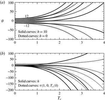
 $(a)$
Evolution of
 $\unicode[STIX]{x1D703}$
versus scaled time
 $T_{c}$
for different
 $\unicode[STIX]{x1D703}(0)$
values (
 $-12,-6,0,6,12$
) with
 $\text{d}\unicode[STIX]{x1D703}/\text{d}T(0)=0$
, when
 $b=0$
or
 $10$
. The horizontal dashed curve is for
 $\unicode[STIX]{x1D703}(0)=b=0$
.
 $(b)$
Scaled height
 $h$
(thick curves) and skin-friction perturbation
 $\unicode[STIX]{x1D70F}$
/
 $\unicode[STIX]{x1D6FF}$
at the trailing edge (dotted curves) versus
 $T_{c}$
, for
 $b$
zero, under the same conditions as in
 $(a)$
. The dotted curves are the thinner ones in
 $(b)$
;
 $\unicode[STIX]{x1D703}(0)=-12$
gives the top curves in
 $h$
,
 $\unicode[STIX]{x1D70F}/\unicode[STIX]{x1D6FF}$
whereas 12 gives the bottom ones.

Solutions of (5.3)–(5.5) are shown in figure 3(a,b) and cover a range of initial conditions as well as parameter values with regard to the underbody thickness and their influences on the long-term responses. Here
 $\hat{M}=1$
,
 $\hat{I} =0.2$
throughout. Figure 3(a) includes plots of
 $\unicode[STIX]{x1D703}$
versus scaled time and figure 3(b) shows the temporal variation of the corresponding h and skin-friction values at the trailing edge. These solutions are explicitly
 $$\begin{eqnarray}\displaystyle & \displaystyle \unicode[STIX]{x1D703}=D_{1}\exp (T_{c})+D_{2}\exp (-T_{c})-D_{3}, & \displaystyle\end{eqnarray}$$
 $$\begin{eqnarray}\displaystyle & \displaystyle h-h(0)-T_{c}\frac{\text{d}h}{\text{d}T_{c}}(0)=D_{4}(\exp (T_{c})-1)+D_{5}(\exp (-T_{c})-1)+D_{6}T_{c}^{2}, & \displaystyle\end{eqnarray}$$
while
 $h_{K}$
follows directly from (5.5), (5.6). The constants
 $D_{1}$
,
 $D_{2}$
depend on the initial conditions,
 $T=[\hat{I} \unicode[STIX]{x1D6FE}^{-1}2^{5}3^{-4}(35)]^{1/2}T_{c}$
,
 $b=[5^{-2}(91)]D_{3}$
,
 $D_{4}=\unicode[STIX]{x1D705}s_{1}D_{1}$
,
 $D_{5}=\unicode[STIX]{x1D705}s_{1}D_{2}$
,
 $D_{6}=\unicode[STIX]{x1D705}(s_{2}-s_{1}D_{3})/2$
where
 $s_{1}=-9/112$
,
 $s_{2}=9b/(560)-\hat{M}{\hat{g}}$
,
 $\unicode[STIX]{x1D705}=2^{5}(35)3^{-2}\hat{I} /\hat{M}$
. The results point to unbounded growth emerging. The long-term behaviour in every case takes the form, with constants having subscript
 $d$
,
 $$\begin{eqnarray}\displaystyle \left[h,\unicode[STIX]{x1D703},K\right]=\left[h_{d},\unicode[STIX]{x1D703}_{d},K_{d}\right]e^{QT}. & & \displaystyle\end{eqnarray}$$
The constant growth rate
 $Q$
is found to have four possible roots with the values of the coefficients
 $[h_{d},\unicode[STIX]{x1D703}_{d},K_{d}]$
determined by the initial conditions on
 $h$
,
 $\unicode[STIX]{x1D703}$
,
 $\text{d}h/\text{d}t$
,
 $\text{d}\unicode[STIX]{x1D703}/\text{d}t$
. These roots (characteristic values) come from replacing
 $\text{d}^{2}/\text{d}T^{2}$
by
 $Q^{2}$
of course in the unforced problem, and at least one root has positive real part
 $Q_{r}$
which indicates temporal unbounded growth or instability. In fact the roots are explicitly
 $$\begin{eqnarray}\displaystyle Q=\pm \frac{9}{4}\left\{\frac{\unicode[STIX]{x1D6FE}}{70\hat{I} }\right\}^{1/2},\,0\,(\text{twice}). & & \displaystyle\end{eqnarray}$$
The two zero roots correspond to
 $\unicode[STIX]{x1D703}$
identically zero with
 $h$
being
 $\hat{a}+\hat{b}T$
for constants
 $\hat{a}$
,
 $\hat{b}$
, but at large
 $T$
the
 $Q_{r}>0$
root dominates (5.8) in virtually every case. The roots all together depend only on the parameters
 $\hat{I}$
(moment of inertia),
 $\unicode[STIX]{x1D6FE}$
(viscous response) whereas the initial conditions and both
 $\hat{M}$
and
 $\hat{I}$
control
 $h_{d}$
, thereby bringing in the influences of the body mass. The influence of gravity
 ${\hat{g}}$
is negligible relative to (5.8). Overall exponential growth
 $(Q_{r}>0)$
accompanied by linear growth corresponding to (5.8), (5.9) dominates at large times.
Physically the non-alignment due to the scaled angle
 $\unicode[STIX]{x1D703}$
varying plays the decisive role in the exponential growth above as (5.3)–(5.5) show. The presence of fluid flow and hence fluid–body interaction accentuates this: a slight increase in
 $\unicode[STIX]{x1D703}$
induces pressure that is negative underneath the body compared with on top and biased towards the front of the body, when combined with the trailing edge constraint, which then yields positive torque and hence forces
 $\unicode[STIX]{x1D703}$
to increase further and so on, leading to unbounded growth. There is no so-called added mass effective here since the fluid flow remains quasi-steady. Moreover the increasing
 $\unicode[STIX]{x1D703}$
causes the relative height factor
 $h_{K}$
to decrease in view of the relationship (5.5) which is associated with the trailing edge constraint. So the combined influence on the vertical motion is to cause the body to accelerate towards the wall, from (5.3), giving a positive gravity effect. Thus with this initial condition the body rotates anticlockwise and approaches the wall. (An initially decreasing displacement in the lower part of the core broadly gives rise to a decreasing pressure there due to the viscous wall-layer response and it provokes no pressure on top. Hence the pressure difference rises, causing the body to accelerate towards from the wall. This adds to the decreasing displacement of the wall layer and core and so boosts the downward trend.) A similar self-perpetuating growth arises if the trend in
 $\unicode[STIX]{x1D703}$
starts downward, yielding a negative gravity effect; the body then rotates clockwise and departs from the wall. We remark that the basic height
 $y_{0}$
has no effect in any case in the current regime as inferred from the displacement properties in (2.3)–(2.5) and similarly the body length
 $L$
has no qualitative effect here. The main feature in the present range is clearly the growth (5.8), which comes from the influence of the torque on the scaled angle.
6 Stabilising features
Given the instability that is seen to occur in a boundary layer or channel flow in the configuration of the previous section we now examine the possibility of there being stabilising mechanisms. Three are found, as described in §§ 6.1–6.3 below.
6.1 Front-heavy body
When the centre of mass of the thin rigid body is in a general position
 $X=\unicode[STIX]{x1D6E5}$
rather than just at the midway point as assumed in the previous sections then most of the preceding analysis remains intact. Here
 $0<\unicode[STIX]{x1D6E5}<1$
. In fact the working in §§ 2–3 is unaltered except that
 $(X-1/2)$
is replaced by
 $(X-\unicode[STIX]{x1D6E5})$
in the scaled torque (3.7), (3.9) and the changes in § 5 are then associated with the influence of
 $\unicode[STIX]{x1D6E5}$
through the torque
 $C_{M}$
in (5.4). Consequently, for the case of the parabolic underbody shape, (5.4) becomes
 $$\begin{eqnarray}\displaystyle \hat{I} \frac{\text{d}^{2}\unicode[STIX]{x1D703}}{\text{d}T^{2}}=9\unicode[STIX]{x1D6FE}\{J_{1}\unicode[STIX]{x1D703}+J_{2}b\}, & & \displaystyle\end{eqnarray}$$
where the constants
 $J_{1}$
,
 $J_{2}$
are given by
 $$\begin{eqnarray}J_{1}=3^{2}2^{-5}7^{-1}\left[\frac{1}{5}+2\left(\unicode[STIX]{x1D6E5}-\frac{1}{2}\right)\right],\quad J_{2}=3^{2}2^{-4}7^{-2}5^{-1}\left[\frac{2^{-1}5^{2}}{13}-7\left(\unicode[STIX]{x1D6E5}-\frac{1}{2}\right)\right],\end{eqnarray}$$
after use of (5.5). The value of the coefficient
 $J_{1}$
is important since it controls the character of the solution
 $\unicode[STIX]{x1D703}$
of (6.1) with the variation of the angle
 $\unicode[STIX]{x1D703}$
itself dictating whether the whole fluid–body system exhibits unbounded growth or not. Here the first equation in (6.2) shows that there is a critical value
 $\unicode[STIX]{x1D6E5}_{0}$
of the streamwise position
 $\unicode[STIX]{x1D6E5}$
of the centre of mass, namely
 $$\begin{eqnarray}\displaystyle \unicode[STIX]{x1D6E5}_{0}={\textstyle \frac{2}{5}}, & & \displaystyle\end{eqnarray}$$
such that
 $J_{1}$
is positive for
 $\unicode[STIX]{x1D6E5}$
above
 $\unicode[STIX]{x1D6E5}_{0}$
and negative below
 $\unicode[STIX]{x1D6E5}_{0}$
. The former range indicates instability as before whereas the range
 $\unicode[STIX]{x1D6E5}<\unicode[STIX]{x1D6E5}_{0}$
suggests stability is possible.
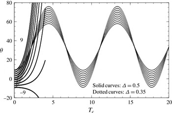
Angle
 $\unicode[STIX]{x1D703}$
versus
 $T_{c}$
for
 $\unicode[STIX]{x1D703}$
initial values (
 $-9$
to
 $9$
in steps of 2) as indicated when centre-of-mass position
 $\unicode[STIX]{x1D6E5}$
is changed from
 $0.5$
(solid curves) to
 $0.35$
(dotted curves). Here
 $b=8$
. On the dotted curves, which are the ones showing clear oscillation, the maximum amplitudes are those for an initial theta of
 $-0.9$
whereas the minimum amplitudes are for the initial value
 $9$
.

The main results for the evolution of the angle
 $\unicode[STIX]{x1D703}$
are shown in figure 4, for a thickness parameter
 $b=8$
. They are subject to the initial conditions of given
 $\unicode[STIX]{x1D703}(0)$
and zero
 $\text{d}\unicode[STIX]{x1D703}/\text{d}T$
at zero time and so, with
 $T_{c}$
denoting
 $Q_{1}T$
, they correspond to the solutions
 $$\begin{eqnarray}\displaystyle & \displaystyle \unicode[STIX]{x1D703}=\{\unicode[STIX]{x1D703}(0)+J_{2}bJ_{1}^{-1}\}\cosh (Q_{1}T)-J_{2}bJ_{1}^{-1}\quad \text{for }\unicode[STIX]{x1D6E5}>\unicode[STIX]{x1D6E5}_{0}, & \displaystyle\end{eqnarray}$$
 $$\begin{eqnarray}\displaystyle & \displaystyle \unicode[STIX]{x1D703}=\frac{9\unicode[STIX]{x1D6FE}J_{2}bT^{2}}{2\hat{I} }+\unicode[STIX]{x1D703}(0)\quad \text{for }\unicode[STIX]{x1D6E5}=\unicode[STIX]{x1D6E5}_{0}, & \displaystyle\end{eqnarray}$$
 $$\begin{eqnarray}\displaystyle & \displaystyle \unicode[STIX]{x1D703}=\{\unicode[STIX]{x1D703}(0)+J_{2}bJ_{1}^{-1}\}\cos (Q_{2}T)-J_{2}bJ_{1}^{-1}\quad \text{for }\unicode[STIX]{x1D6E5}<\unicode[STIX]{x1D6E5}_{0}, & \displaystyle\end{eqnarray}$$
as
 $\unicode[STIX]{x1D6E5}$
,
 $\unicode[STIX]{x1D703}(0)$
are varied. Here
 $Q_{1}=3(\unicode[STIX]{x1D6FE}J_{1}/\hat{I} )^{1/2}$
,
 $Q_{2}=3(-\unicode[STIX]{x1D6FE}J_{1}/\hat{I} )^{1/2}$
. In essence the non-trivial eigenvalues
 $Q$
in (5.9) are replaced by
 $\pm 3(\unicode[STIX]{x1D6FE}J_{1}/\hat{I} )^{1/2}$
but allowing for subcritical values of
 $J_{1}$
being negative. The change in character from exponential growth to bounded oscillation as
 $\unicode[STIX]{x1D6E5}$
is reduced from above critical to below is highlighted by the figure (which has
 $\unicode[STIX]{x1D6E5}$
equal to 0.5 and 0.35) and is as expected from (6.1). It is also sensible physically because as far as the torque is concerned the front loading of the body associated with decreasing
 $\unicode[STIX]{x1D6E5}$
below
 $1/2$
reduces the moment of the more rapidly varying pressure forces near the leading edge (compared with those towards the rear of the body) and this happens to such an extent when
 $\unicode[STIX]{x1D6E5}$
is less than
 $\unicode[STIX]{x1D6E5}_{0}$
that the effect suppresses any growth in the angle
 $\unicode[STIX]{x1D703}$
. It is worth remarking that the alteration in the position of the centre of mass required for stabilisation is predicted as 10 % only, according to (6.3), compared with the original central position; this alteration in conditions is notably small.
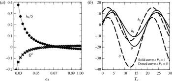
 $(a)$
Eigenvalue
 $Q^{2}$
(crosses) and relative height
 $h_{K}$
(dots) versus flexibility parameter
 $e_{2}$
. Effectively
 $P_{0}$
is zero. The changes in sign of
 $Q^{2}$
at (6.5) (approx.
 $0.062$
) and of
 $h_{K}$
at
 $e_{2}$
approx
 $0.077$
are noted.
 $(b)$
 $\unicode[STIX]{x1D703}$
,
 $h_{K}$
versus
 $T_{c}$
for
 $P_{0}$
of
 $1$
,
 $5$
when
 $e_{2}$
is
 $0.01$
.

6.2 Flexible section in body
If the underbody is flexible then again significant changes in the fluid–body interactive behaviour may be produced. The possibility arises from the effects of varying
 $b$
in § 3 (see figure 2
a,b) and is examined in detail below. In this context for the boundary layer the governing equations of § 2, § 3 mostly remain valid in their quasi-steady form but the underbody shape becomes unknown; so (3.1) for instance applies no longer. Instead the shape is related to the unknown underbody pressure
 $P(X,T)$
by means of a flexible surface equation (Cox & Mason Reference Cox and Mason1971; Carpenter & Garrad Reference Carpenter and Garrad1985; Guneratne & Pedley Reference Guneratne and Pedley2006; Pruessner & Smith Reference Pruessner and Smith2015). If
 $e_{2}$
is the scaled longitudinal tension of the underbody surface and
 $P_{0}$
is the constant scaled base pressure inside the body relative to the incident pressure, then the equations and boundary conditions are
 $$\begin{eqnarray}\displaystyle & \displaystyle e_{2}\frac{\unicode[STIX]{x2202}^{2}f_{u}}{\unicode[STIX]{x2202}X^{2}}=P_{0}-P, & \displaystyle\end{eqnarray}$$
 $$\begin{eqnarray}\displaystyle & \displaystyle f_{u}(0,T)=f_{u}(1,T)=0. & \displaystyle\end{eqnarray}$$
See the Pruessner & Smith (Reference Pruessner and Smith2015) system for a different setting. Here the signs in (6.7) reflect the property that a flow pressure higher than the base pressure provokes a negative curvature and thus an overall rise in the underbody shape. The ensuing interaction is thus controlled by (3.6), (3.7), (5.1), (5.2) with (6.7) and (6.8), as well as the general results (A 5), (A 6) in appendix A, for the prediction of
 $(\unicode[STIX]{x1D703},h,h_{K},P,f_{u})$
as time increases.
Solutions of the flexible body interaction yield a supercritical or subcritical response giving unbounded growth or bounded oscillation similar to that in the previous subsection. For comparison purposes we show in figure 5(a) the results of the
 $Q$
-approach in which a behaviour (5.8) is supposed as in § 5, such that
 $\hat{I} Q^{2}\unicode[STIX]{x1D703}_{d}$
replaces the left-hand side of (5.2). The value of
 $\unicode[STIX]{x1D703}_{d}$
can be normalised to unity by working with
 $(h,h_{K},P,f_{u})/\unicode[STIX]{x1D703}_{d}$
, the value of
 $\unicode[STIX]{x1D706}$
can likewise be taken as unity without loss of generality and the value of
 $P_{0}$
is negligible in the cases of exponential growth. The figure gives the prediction for
 $Q^{2}$
and the representative quantity
 $h_{K}$
as
 $e_{2}$
is varied. Although at larger
 $e_{2}$
the response
 $Q^{2}$
is always positive, as
 $e_{2}$
is decreased a form of resonance comes into action in which the response is enhanced (Pruessner & Smith Reference Pruessner and Smith2015) and this leads to successive changes in the sign of
 $Q^{2}$
. The critical value of the scaled longitudinal tension
 $e_{2}$
below which bounded behaviour is first found is
 $$\begin{eqnarray}\displaystyle e_{2}=e_{20}=\text{approx. }0.062. & & \displaystyle\end{eqnarray}$$
Hence stabilisation is again apparent.
Figure 5(b) presents results for the temporal evolution of the angle and the relative height factor
 $h_{K}$
at the subcritical value
 $e_{2}=0.01$
. For given flexible material properties a decrease of
 $e_{2}$
to a subcritical value for example is caused by an increase in the incident flow strength. The results agree with those in figure 5(a) in that continued oscillations are found to occur with the amplitude and frequency depending on the parameter values, namely
 $P_{0}$
of
 $1$
and
 $5$
in this case, for the subcritical range.
6.3 Streamwise movement of the body
As the velocity
 $V_{c}$
of the body is increased in the streamwise direction it first affects the fluid–body interaction significantly in the boundary-layer case when
 $V_{c}$
is of order
 $L^{1/3}$
, due to the background flow velocity in (2.7) (Smith & Johnson Reference Smith and Johnson2016). The influence on the core flow is negligible at this stage.
Above that size, for the range of body velocities
 $L^{1/3}\ll V_{c}\ll 1$
, the scaled central problem (2.17)–(2.21) is altered by having a term
 $-C$
(
 $=-V_{c}L^{-1/3}$
) due to advection in the inertial contribution in place of the term
 $\unicode[STIX]{x1D706}Y$
due to shear in (2.18). The influence of
 $V\unicode[STIX]{x1D706}$
is also suppressed then. In effect
 $Y$
is scaled by a factor
 $C^{-1/2}$
, leading to
 $f^{+}$
,
 $f^{-}$
,
 $K$
,
 ${\hat{h}}$
,
 $\hat{\unicode[STIX]{x1D703}}$
all being of order
 $P/C$
with the size of
 $P$
to be found. The time scale
 $T$
must decrease like
 $C^{-1/2}$
. The present assumption is that
 $\hat{M}$
,
 $\hat{I}$
are of order unity, as are
 $\unicode[STIX]{x1D706}$
,
 $X$
. The wall layer thereby becomes a classical layer subjected to an upstream moving wall condition, with the influence of the underlying shear proportional to
 $\unicode[STIX]{x1D706}$
being diminished. To leading order the fluid-flow equations are
 $$\begin{eqnarray}\displaystyle & \displaystyle U=\unicode[STIX]{x1D6F9}_{Y}, & \displaystyle\end{eqnarray}$$
 $$\begin{eqnarray}\displaystyle & \displaystyle V=-\unicode[STIX]{x1D6F9}_{X}, & \displaystyle\end{eqnarray}$$
 $$\begin{eqnarray}\displaystyle & \displaystyle -CU_{X}=-P_{X}+U_{YY}, & \displaystyle\end{eqnarray}$$
confirming that the major advection here is in the negative
 $X$
-direction. This classical sub-boundary layer acts as if with prescribed pressure except that the pressure is itself evolving. The behaviour in the outer reaches of the layer implies
 $$\begin{eqnarray}\displaystyle P=\unicode[STIX]{x1D706}C\left\{K-f_{u}(X)-h-(X-{\textstyle \frac{1}{2}})\unicode[STIX]{x1D703}\right\}+\hat{E} & & \displaystyle\end{eqnarray}$$
for the pressure where
 $\hat{E}$
is a constant, from (2.20) with (6.12). The response here is predominantly inviscid.
In consequence the body motion balances (5.1), (5.2) of the fluid–body interaction give successively
 $$\begin{eqnarray}\displaystyle & \displaystyle \hat{M}\frac{\text{d}^{2}h}{\text{d}T^{2}}=\unicode[STIX]{x1D706}C(K-h)+ & \displaystyle \hat{E}-\hat{M}{\hat{g}},\end{eqnarray}$$
 $$\begin{eqnarray}\displaystyle & \displaystyle \hat{I} \frac{\text{d}^{2}\unicode[STIX]{x1D703}}{\text{d}T^{2}}=-\frac{\unicode[STIX]{x1D706}C}{12}\unicode[STIX]{x1D703}, & \displaystyle\end{eqnarray}$$
after integration. This is strictly for an underbody shape
 $f_{u}$
of zero. A non-zero shape
 $f_{u}$
merely adds at most a constant to (6.14), (6.15) while if
 $f_{u}$
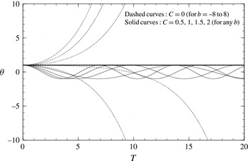
is symmetric about the centre of mass, as in the parabolic case of (3.1), then (6.15) remains unchanged. The decisive equation in any case is that for the angular momentum of the body in (6.15). Results are presented in figure 6 for varying positive
 $C$
values and compared with the corresponding results for the previous
 $C=0$
configuration, emphasising the stabilising effect of the body movement.
Angle
 $\unicode[STIX]{x1D703}$
versus scaled time for initial value
 $\unicode[STIX]{x1D703}(0)=1$
when body has scaled streamwise velocity
 $C=0$
(with
 $b$
of
 $-8,-4,0,4,8$
, from the bottom to the top dashed curve respectively) or
 $C=0.5,1,1.5,2$
(for any
 $b$
value).

Physically the fluid motion part of the present interaction yields a pressure contribution proportional to the flow width, a result which is akin to that in Smith & Daniels (Reference Smith and Daniels1981) in a different context, and the coupling with the body motion part then produces oscillations in
 $\unicode[STIX]{x1D703}$
for any positive body velocity
 $C$
. Thus in (6.13) an increase in
 $\unicode[STIX]{x1D703}$
induces a pressure decrease downstream of the centre of mass of the body, which here is at the midway location, whereas the pressure upstream is increased, and this acts to reduce the torque on the body. In turn the angular acceleration is therefore reduced in (5.2) or explicitly as in (6.15) which tends to decrease the angular velocity and so the movement is stabilised, as in simple harmonic motion. The oscillation frequency increases with increasing
 $C$
. The reduced form in (6.13) and hence in (6.14)–(6.15) is related to the findings from the response of the Tietjens function in Smith & Johnson (Reference Smith and Johnson2016) and it is noted that a response similar to that in (6.10)–(6.14) occurs for the channel-flow case of § 4 at increased body velocity.
7 Further discussion
The results altogether have shown first that over the present scales the fluid/body interaction for a single finite body moving freely is the same in a boundary layer as in a channel flow. Second, the interaction can be unstable. Third however there are at least three factors that can stabilise the interplay by changing the decisive balance of angular momentum of the body. These three are a shift forward in the location of the centre of mass, a flexible underside in the body and a slight streamwise movement of the body. Fourth, the overall effects produced are independent of the lateral position of the body within the core over the current range of scales. The considerable implications from this are as follows.
The waves (in stabilised cases) and the instabilities (otherwise) studied in this work rely on two-way interplay between the body movements and the surrounding fluid motions in the boundary layer or channel flow. All of the stabilising measures considered seem to make sense physically as well as indicating potential safety measures in certain applications. Front loading of a body in a relatively fast flow of fluid in order to mitigate against instability is intuitively sensible and also agrees with the reduced torque from pressures near the leading edge. Using wall or body flexibility to absorb energy and suppress instability is also intuitively reasonable as well as subject to delicate balances between shape, pressure and torque. Moving the body along with the fluid may similarly appear sensible physically and is in keeping with the change induced in the pressure–displacement interaction which forms part of the whole fluid–body interplay. In detail however the shift in the location of the centre of mass needed for stabilisation due to front-loading is surprisingly small, being only 10 %, i.e. a shift from the 50 % midway location to the 40 % location. Likewise the body velocity needed for stabilisation due to streamwise movement is notably small, being at any rate between the order of the viscous wall-layer speed and order unity relative to the incident speed in the boundary layer and similarly small in terms of the underlying velocity in a channel flow. This is for rightwards movement in figure 1(a,b). If the body is moved leftwards then the reversed convection yields increased instability instead. Figure 6 for example illustrates the point about mitigation in terms of the rightwards body movement. The mitigations or stabilisations here have varied relevance in the applications described in the introduction to the paper. We remark also that in the stable cases the perturbation in body orientation (denoted
 $\unicode[STIX]{x1D703}$
) oscillates in time whereas that in distance from the wall (denoted
 $h$
) increases linearly with time but the direction remains dependent on the initial conditions.
Neither the lateral location nor the streamwise length of the body has any qualitative effect at leading order within the present range of concern shown in figure 1(a,b). The current work and that in Smith & Johnson (Reference Smith and Johnson2016) imply that apart from the stabilising measures above most body lengths can lead to unstable fluid–body interaction with viscous–inviscid shear flow, which appears to contrast significantly with properties at low flow rates. On the other hand the question of what happens when the body is nearer a wall, especially inside a viscous wall layer, remains to be studied. Interesting further problems arise also if the body length is reduced to the triple-deck size or enhanced to the development length scale associated respectively with the lower and upper restrictions of the theory (see (2.1)) in the context of a boundary layer and likewise for a channel flow (see just before (4.1)). Increased ellipticity is bound to arise for shorter lengths in view of the length scales of upstream influence. Related to the upstream influence in channel flow a low axial speed has a prime effect only in altering upstream effects ahead of the leading edge and these alterations take place over a length scale of order
 $R^{1/7}$
, much less than the body length, see (4.1). The lateral pressure gradient becomes important then yielding an extension of the original
 $\exp (\bar{\unicode[STIX]{x1D705}}R^{-1/7}x)$
mechanism but an additional mechanism discussed in an appendix of Smith (Reference Smith1984) on upstream influence in separating flow is found to enter the reckoning. These mechanisms are associated with zero-pressure-gradient and zero-displacement viscous layers respectively when the velocity continues to increase. A similar process arises for the boundary layer but is a little more complicated because of algebraic upstream influence.
Restrictions on the theory due to lateral location and length scales have been mentioned, and other restrictions concern two-dimensionality, the Reynolds-number (
 $Re$
) range, the streamwise body velocity and the body thickness for example. The time scale assumption imposes the limitation that for the boundary layer setting the density ratio
 $\unicode[STIX]{x1D70C}_{B}^{\ast }/\unicode[STIX]{x1D70C}^{\ast }\gg ReL^{2/3}\unicode[STIX]{x1D716}^{-2}$
, which is large, and indeed time scales other than those examined here are of additional concern. In the case of an ice shard in a boundary layer of air the density ratio is of the order
 $10^{3}$
typically which may exceed the expression above. This depends on local boundary-layer properties: characteristic values are
 $Re$
of
 $10^{3}$
to
 $10^{5}$
say, length
 $L$
of
 $10^{-2}$
at least,
 $\unicode[STIX]{x1D716}^{-2}$
of approximately
 $5$
, which give a similar or smaller order of magnitude but the skin-friction factor
 $\unicode[STIX]{x1D706}$
can effectively reduce or increase the value of
 $\unicode[STIX]{x1D716}$
by altering the viscous wall-layer thickness. Further, the body Reynolds number
 $Re_{p}$
based on body length may be as low as
 $10^{2}$
to
 $10^{3}$
for the above range and this covers the range of experimental values of the critical
 $Re_{p}$
observed (Petrie et al.
Reference Petrie, Morris, Bajwa and Vincent1993; Schmidt et al.
Reference Schmidt, Young and Benard2010) for spherical particles in a laminar boundary layer. The work may seem contentious in view of all the assumptions made but it does support the possibility of extensive flow destabilisation due to interaction, as well as contrasting stabilisation measures which include front loading, flexible bodies and favourable streamwise movement in particular applications. These features might be helpful or of interest experimentally and in terms of direct simulations and they also provide a set of analytical case studies potentially useful for comparisons.
The effects of further increased body velocity in the streamwise direction examined in § 6.3 and the last-but-one paragraph and of increased disturbance amplitude are now addressed. The former provides a springboard for considering body velocities of order unity, a regime which is perhaps of most practical interest. Clearly a critical layer occurs then as in Smith & Johnson (Reference Smith and Johnson2016), and this is without an inflection point in the cases considered so far. We have focused on small disturbances and these produce linear interactions which allow more progress analytically. Nonlinear cases occur if the amplitude parameter (
 $\unicode[STIX]{x1D716}$
) is increased slightly, with the viscous wall layer of § 2 first becoming nonlinear through an inertial response of the form
 $UU_{X}+VU_{Y}$
essentially: cf. (2.18). A combination of both effects produces in addition the boundary condition
 $U\sim \unicode[STIX]{x1D706}Y-C+\unicode[STIX]{x1D706}A$
at large values of the wall-layer coordinate
 $Y$
. As the scaled body velocity
 $C$
increases the shear influence
 $\unicode[STIX]{x1D706}Y$
diminishes, pointing to the relation
 $P=-1/2(C-\unicode[STIX]{x1D706}A)^{2}$
to within an additive function of time. This is coupled with the relation involving
 $A$
,
 $\unicode[STIX]{x1D703}$
in § 3 (see also appendix A) and the body angular momentum equation in § 5 involving
 $P$
,
 $\unicode[STIX]{x1D703}$
. The nonlinear response then is overwhelmingly inviscid but has the potential for viscous sublayer eruptions. That is based initially on the issue of separation in the quasi-steady classical viscous layer close to the wall when the amplitude is sufficiently large. It might suggest a classical Goldstein singularity but with account taken that the free movement of the body renders the pressure unknown and there is interplay with the original viscous–inviscid interactive wall layer (cf. Smith & Daniels Reference Smith and Daniels1981). Further study is again necessary here.
Acknowledgements
Thanks are due to R. Gent and R. Moser at AeroTex, R. Lewis at TotalSim, S. Bee and M. Honeywood at Sortex-Buhler and colleagues R. Bowles, E. Johnson, N. Ovenden and S. Timoshin for helpful discussions on body and particle movement in near-wall shear flow. Support from EPSRC (UK) through grant numbers GR/T11364/01, EP/D069335/1, EP/G501831/1, EP/H501665/1, EP/H500278/1 during part of this research is gratefully acknowledged.
Appendix A. Detailed solving and results for a general body shape
The viscous parts in (2.17)–(2.21) can be treated as follows. Taking a Fourier transform in
 $X$
with transformed variable
 $\unicode[STIX]{x1D6FC}$
converts (2.17)–(2.18) to Airy’s equation for the transformed shear stress
 $\unicode[STIX]{x1D70F}^{(F)}$
as in Stewartson (Reference Stewartson1970), Smith (Reference Smith1973) with
 $(.)^{(F)}$
denoting the Fourier transform and
 $\unicode[STIX]{x1D70F}$
denoting
 $U_{Y}$
. We then apply the boundary conditions on
 $\unicode[STIX]{x1D70F}_{Y}^{(F)}$
at
 $Y=0$
and on the integral of
 $\unicode[STIX]{x1D70F}^{(F)}$
with respect to
 $Y$
from
 $0$
to
 $\infty$
to obtain the transforms of the pressure and skin-friction solutions
 $$\begin{eqnarray}\displaystyle & \displaystyle P^{(F)}(\unicode[STIX]{x1D6FC})=3(\text{i}\unicode[STIX]{x1D6FC})^{-1/3}\unicode[STIX]{x1D706}^{5/3}A^{(F)}(\unicode[STIX]{x1D6FC})A_{i}^{\prime }(0), & \displaystyle\end{eqnarray}$$
 $$\begin{eqnarray}\displaystyle & \displaystyle \unicode[STIX]{x1D70F}^{(F)}(\unicode[STIX]{x1D6FC},0)=(\text{i}\unicode[STIX]{x1D6FC})^{2/3}\unicode[STIX]{x1D706}^{-1/3}P^{(F)}(\unicode[STIX]{x1D6FC})A_{i}(0)/A_{i}^{\prime }(0). & \displaystyle\end{eqnarray}$$
Here
 $A(X)=K-f_{u}(X)-h-(X-1/2)\unicode[STIX]{x1D703}$
is known over the body length
 $0<X<1$
although unknown in the wake
 $X>1$
. The form (A 1) allows the pressure response in particular to be expressed explicitly in terms of the displacement response, or vice versa. Also
 $A=0$
in
 $X<0$
owing to the lack of upstream influence but
 $A$
jumps across
 $X=0\pm$
in general whereas
 $P=0$
in
 $X<0$
and
 $P=0$
at
 $X=0+$
. Inversion of (A 1) thus leads to the direct relation (Pruessner & Smith Reference Pruessner and Smith2015)
 $$\begin{eqnarray}\displaystyle P(X)=\unicode[STIX]{x1D6FE}\int _{0}^{X}\left\{f_{u}(S)+h+\left(S-{\textstyle \frac{1}{2}}\right)\unicode[STIX]{x1D703}-K\right\}(X-S)^{-2/3}\,\text{d}S,\quad \text{for }0<X<1, & & \displaystyle\end{eqnarray}$$
where the constant
 $\unicode[STIX]{x1D6FE}=0.289838(\unicode[STIX]{x1D706})^{5/3}$
is positive. The form (A 2) leads to the result (3.5). The parabolic nature of (A 3) on its own in the positive
 $X$
-direction is noted, i.e. the integral runs forward from zero to
 $X$
, although the entire system here, i.e. (2.17)–(2.21), remains elliptic between
 $X=0$
,
 $1$
because of
 $K$
. The upstream match with zero pressure is incorporated in (A 3), while the downstream effect or wake is discussed near the end of the present section.
Given (A 3) the pressure condition (2.21) requires
 $$\begin{eqnarray}\displaystyle 3K=\int _{0}^{1}\left\{f_{u}(S)+h+\left(S-\frac{1}{2}\right)\unicode[STIX]{x1D703}\right\}(1-S)^{-2/3}\,\text{d}S, & & \displaystyle\end{eqnarray}$$
determining
 $K$
whenever
 $f_{u}$
,
 $h$
,
 $\unicode[STIX]{x1D703}$
are known. We therefore obtain the pressure underneath the body as
 $$\begin{eqnarray}\displaystyle P=\unicode[STIX]{x1D6FE}\{(h-K)i_{1}(X)+\unicode[STIX]{x1D703}i_{2}(X)+i_{3}(X)\}. & & \displaystyle\end{eqnarray}$$
Here
 $i_{1}$
,
 $i_{2}$
and
 $i_{3}$
depend only on
 $X$
; thus
 $i_{1}(X)=3X^{1/3}$
,
 $i_{2}(X)=-3X^{1/3}/2+9X^{4/3}/4$
,
 $i_{3}(X)=\int _{0}^{X}f_{u}(S)(X-S)^{-2/3}\,\text{d}S$
. Also
 $K$
is given by
 $$\begin{eqnarray}\displaystyle K=h+\frac{\unicode[STIX]{x1D703}}{4}+E_{1}, & & \displaystyle\end{eqnarray}$$
where
 $E_{1}=i_{3}(1)/3$
; this result for the quasi-height
 $K$
stems from (A 4).