1. Introduction
The COVID-19 pandemic has been one of the largest global crises in a century, endangering human lives and health and inducing severe economic downturns across the globe. This paper aims to investigate the effects of the pandemic on both the health and macroeconomic outcomes of China. For the Chinese government, the COVID-19 outbreak has constituted a dramatic public health emergency and has undoubtedly been the most severe challenge faced since the establishment of the People’s Republic of China in 1949. During the first wave of the pandemic, it took over a month for China to achieve initial success in curbing the spread of the virus, about two months to bring the daily figure of new domestic cases on the mainland down to single digits, and three months to insulate the center of the epidemic, Wuhan city and the Hubei province, from the disease.
In this paper, we begin by briefly documenting China’s containment policies – including lockdowns, testing, and contact tracing – and present empirical evidence on the role of the online economy in the transmission of the COVID shock to the macroeconomy. We then apply a calibrated SIR-macro model tailored to the Chinese context to identify the key forces driving the dynamics of health and economic outcomes during the COVID-related recession, as well as those underpinning the subsequent recovery of the Chinese economy. The model replicates infections and deaths, along with the behavior of major macroeconomic variables during the period under study.
Our main findings are as follows: (i) The online economy, exemplified by online consumption and remote work (work-from-home, WFH), has played a critical role in mitigating the recession. Specifically, remote work has been especially effective in cushioning the declines in output, employment, and investment, while online consumption has been essential for stabilizing aggregate consumption; (ii) the effectiveness of lockdown implementation has significantly influenced both health and economic outcomes. While stricter and well-enforced lockdowns are more successful in reducing infections and deaths, they also result in larger short-run economic losses; (iii) the timing of lockdowns also matters: early implementation can reduce health costs without worsening the severity of the recession; (iv) large-scale testing and contract tracing are crucial for containing the health impacts of a pandemic. We use these findings, along with the institutional and policy details documented in the appendix to convey two broader messages. First, societal resilience – reflected in digital readiness and effective policy execution – is an important factor in successfully combating a pandemic. Second, our analysis supports the view that sustainable economic recovery depends on restoring public confidence in virus containment (Chetty et al., Reference Chetty, Friedman, Hendren and Stepner2020; Romer, Reference Romer2020), and more generally, that containing the pandemic is a prerequisite for stabilizing the economy (Feng et al. Reference Feng, Wu, Yuan and Zhou2022). Thus, while China’s experience may appear exceptional and not easily replicable, some basic principles of epidemic control – such as the importance of digital readiness, credible containment strategies, and adaptive infrastructure – are likely to hold across institutional contexts and can offer useful insights for other countries facing future epidemic crises.
In the paper, we focus on the economic and health effects of the first wave of the epidemic for two reasons.Footnote 1 First, different waves of the epidemic have been characterized by diverse basic reproduction numbers (R0),Footnote 2 leading to distinct health outcomes. Thus, it is challenging to integrate distinct scenarios into a single model. Second, our analysis implements the perfect foresight method as a solution technique, which requires that agents learn the values of all future shocks. This underlying assumption was widely held during the first wave. In contrast, during subsequent waves, there were changes in the international setting, such as the outbreak of the Russia-Ukraine War and transformations in China’s economic conditions, such as the cooling down of the real estate market. The occurrence of these events would prevent us from fully disentangling the economic impact of the epidemic shock from other shocks.
A large body of literature using SIR-macro models has emerged in response to the COVID19 pandemic, aiming to analyze the interplay between epidemiological dynamics and macroeconomic outcomes. Eichenbaum et al. (Reference Eichenbaum, Rebelo, Trabandt and Koijen2021) extend the canonical SIR model of Kermack and McKendrick (Reference Kermack and McKendrick1927) by introducing the interaction between economic activities and the spread of the virus (see also Chan, Reference Chan2021, and Chen et al., Reference Chen, He, Hsieh and Song2020). Kaplan et al. (Reference Kaplan, Moll and Violante2020) embed a SIR-macro model with ICU constraints into a heterogeneous-agent, incomplete-markets model to examine the distributional effects of the pandemic and associated policies. Hevia, Macera and Neumeyer (Reference Hevia, Macera and Neumeyer2022) use data from Colombia to study the effects of lockdowns and one-time transfers on different income groups. Eichenbaum et al. (Reference Eichenbaum, Rebelo and Trabandt2022) investigate how testing, quarantining and non-pharmaceutical interventions affect both health and economic outcomes (see also Berger et al., Reference Berger, Herkenhoff, Huang and Mongey2022). Goenka and Liu (Reference Goenka and Liu2024) argue that economic epidemiology models are essential for guiding public health policy during a pandemic, as they explicitly capture the interactions between disease transmission and individual behavior – something overlooked by pure epidemiological or economic models, which can lead to misguided policy decisions (see also Acemoglu et al., Reference Acemoglu, Chernozhukov, Werning and Whinston2021 and Atkeson, Reference Atkeson2020).Footnote 3
Our paper contributes to this strand of literature in several ways. First, and most importantly, building on the empirical evidence presented in this paper, we explicitly incorporate the online economy – comprising both online consumption and remote work (WFH) – into the SIR-macro framework. This allows us to study how digital infrastructure can cushion economic downturns during a pandemic. Second, while many existing studies introduce lockdowns as stylized policy shocks, we construct a data-driven lockdown process using the Baidu daily within-city travel intensity index, which captures the actual variation in mobility restrictions across time. This approach enables a more realistic modeling of lockdown intensity and its effects on economic and epidemiological outcomes. Third, in contrast to much of the SIR-macro literature that abstracts from capital accumulation for simplicity, our model includes physical capital dynamics, allowing us to analyze the impact of the pandemic on investment and recovery paths. As emphasized by Boucekkine et al. (Reference Boucekkine, Chakraborty, Goenka and Liu2024), incorporating capital is essential for evaluating recovery dynamics more accurately.
The remainder of the paper is organized as follows. Section 2 documents the containment policies implemented in China, describes the U-shaped recovery of the Chinese economy using weekly data, and presents evidence on the role of the online economy. Section 3 introduces the model, and Section 4 describes the calibration strategy. Section 5 presents the main results, including those from the benchmark model as well as several applications of the model. Section 6 concludes. Additional details – including the epidemic timeline, other containment measures, model assumptions regarding households’ beliefs about their health status, population dynamics, solution methods, and robustness checks – are provided in Online Appendices A-H.
2. China’s response to the COVID-19 epidemic: Containment, online economy, and macroeconomic dynamics
In this section, we review China’s pandemic containment strategy, examine macroeconomic responses, and assess the role of the online economy during the crisis. A detailed chronology of the epidemic and additional containment policies is provided in Appendix A.
2.1 Containment policies and institutional context
To curb the spread of COVID-19, the Chinese government implemented swift and large-scale containment measures. Central among these was a strict lockdown initiated in Wuhan on January 23, 2020. This measure – unprecedented in modern Chinese history – involved sealing off the city, suspending public transport, closing public venues, and restricting movement within residential communities. Similar restrictions were adopted across the Hubei province and in other regions.
To enforce these policies at the local level, China relied on its grid-based community governance structure. Community committees coordinated daily operations, enforced lockdown rules, and facilitated contactless delivery of essential goods. More than 150 million people were placed under home isolation at the peak of the outbreak, necessitating complex logistic coordination between central and local governments and more than 500 enterprises to maintain supplies of food, fuel, and medicine. This highly centralized and community-led implementation was critical in halting virus transmission.
In parallel, China significantly expanded its testing and tracing capacity. By April 2020, all second-tier hospitals and district-level disease control centers were required to conduct nucleic acid testing. Innovative pooled testing strategies, such as the “5-in-1” method, were adopted to improve efficiency.Footnote 4 Authorities used big data and artificial intelligence to trace contacts and assess individual exposure risk, issuing digital health QR codes to manage mobility. These measures enabled rapid containment of new outbreaks and contributed to public reassurance.
While these responses were at times criticized as excessive, epidemiological experts have argued that they were instrumental in containing the epidemic and facilitating a relatively swift economic recovery.
2.2 Macroeconomic dynamics and the role of the online economy
2.2.1 Macroeconomic dynamics
In the face of the COVID-19 pandemic, China prioritized the health and well-being of its citizens over short-term economic gains. This commitment was reflected in the stringent nationwide lockdown that lasted two and a half months and ultimately succeeded in containing the virus. With the epidemic under control, economic activities gradually resumed.
Figure 1 shows the year-on-year growth rates of GDP, total consumption, online consumption, and investment from January 20, 2020 to September 28, 2020.Footnote
5
An advantage of using year-on-year growth rates is that they largely eliminate the effects of seasonality. The data are from the National Bureau of Statistics of China. We transform quarterly or monthly data into weekly data using the quadratic-match sum method. Appendix B provides details of this transformation. The weekly GDP growth rate, depicted by the solid line, reached its lowest point in week 7 at
 $-15.94\%$
. This negative growth rate persisted for 13 weeks before turning slightly positive in week 14 (April 20–27), and GDP growth remained positive thereafter. Similarly, the weekly growth rate of aggregate consumption, shown by the dashed line, bottomed out in week 5 at −27.43%. It stayed negative for 19 weeks and turned positive in week 20 (June 1–8), then continued on an upward path.
The year-on-year growth rates of GDP, total consumption, online consumption, and investment from January 20, 2020 to September 28, 2020.

The solid line with circles shows the year-on-year growth rate of investment at the weekly frequency. Its trough occurred in week 7, at −37.79%. After 17 weeks of negative growth, investment became slightly positive starting week 18 (May 18–25), followed by a moderate upward trend.
The dashed line with circles represents the weekly year-on-year growth rate of online consumption. The lowest point was in week 7, at −14.79%. Growth turned positive in week 10 (March 23–30) and remained consistently positive for the rest of the period. These patterns yield key insights. First, the decline in online consumption was about half that of total consumption, implying a sharper contraction in offline spending. Second, online consumption rebounded much faster than total consumption, underscoring its stabilizing role during the crisis. The next subsections examine this role more systematically, first by analyzing the foundations of China’s online economy and then presenting empirical evidence of its buffering effects.
2.2.2 Development of the online economy before the pandemic
Prior to the COVID-19 pandemic, China’s online economy had already undergone rapid and large scale – albeit uneven – development, supported by three main factors. First, China made substantial investments in digital infrastructure. Between 2015 and 2020, these investments totaled over 1.5 trillion yuan.Footnote 6 According to the Digital China Development Report (2020), released by the Cyberspace Administration of China, China had become the global leader in digital infrastructure, building the world’s largest fiber-optic and 4G/5G networks.Footnote 7 Fixed broadband household penetration rose from 52.6% in 2015 to 96% in 2020, while mobile broadband user penetration increased from 57.4% to 108%.Footnote 8 In terms of 5G network construction, China ranked first globally in both speed and scale of deployment, establishing 718,000 base stations and over 200 million terminal connections by 2020. The number of internet users increased from 688 million in 2015 to 989 million in 2020, while the internet penetration rate rose from 50.3% to 70.4% over the same period.Footnote 9 This rapid expansion in user access, combined with extensive infrastructure investment, enabled the online economy (e.g. WFH) to operate with minimal disruption during the pandemic.
Second, China developed a sophisticated e-commerce ecosystem, characterized by vertically integrated platforms, seamless digital payments, and efficient logistics. Major firms like Alibaba and JD.com manage end-to-end supply chains – from AI-based inventory to last-mile delivery. Ubiquitous mobile payments (e.g., Alipay and WeChat Pay) facilitate over 98% of all transactions. During the pandemic, these platforms sustained over 90% operational capacity, supporting “contactless consumption” and maintaining household access to essential goods.
Third, consumer behavior reinforced this digital shift. Unlike many Western consumers who prioritize privacy, Chinese consumers prioritize convenience over absolute privacy protection. They are willing to make a controlled trade-off of their privacy rights in exchange for digital benefits. This accelerated the adoption of livestreamed shopping, telemedicine, and online education during lockdowns.
Together, these factors – digital infrastructure, platform capacities, and consumer adaptability – positioned China as the global leader in online retail. According to the United Nations Conference on Trade and Development (UNCTAD), seven countries – Australia, Canada, China, Korea, Singapore, the United Kingdom, and the United States – accounted for 65% of global Business-to-Consumer (B2C) e-commerce in 2019. China led the group in 2018–2020, with online retail sales of
 $\$$
1,060.4 billion,
 $\$$
1,233.6 billion and
 $\$$
1,414.3 billion, respectively, amounting to over half of the total online retail sales among the seven countries.
However, the development of online retail has not been uniform across China. A joint report by the World Bank and Alibaba Group shows significant regional disparities. In 2017, online purchases accounted for 49% of retail sales in Shanghai, 44% in Beijing, 36% in Guangzhou, and 35% in Zhejiang – all coastal and economically advanced regions. In contrast, seven inland provinces reported less than 2% online retail share.Footnote
10
China’s ranking in the 2019 UNCTAD B2C E-commerce Index further highlights this discrepancy.Footnote
11
While Switzerland ranked first, China placed
 $55^{th}.$
This relatively low ranking reflects the index’s emphasis on readiness factors such as internet access, secure servers, financial inclusion, and postal reliability – rather than the scale of e-commerce itself. For example, in 2019, China ranked only
 $87^{th}$
in internet penetration and
 $33^{rd}$
in online shopping penetration.
2.3 Evidence from a difference-in-differences test
We provide evidence on the influence of the online economy (digital development) on the transmission of the COVID shock to Chinese households’ consumption using a difference-in-differences approach. Our goal is to verify whether the access of Chinese households to the online economy influenced, and possibly mitigated, their response to the shock induced by the COVID pandemic. To this end, we conduct a difference in difference estimation, in which we test the response of Chinese households’ consumption to (a proxy for) the COVID shock, accounting for the level of digital development at the provincial level. Consistent with the above discussion, Lin et al. (Reference Lin, Zhang, Hou and Li2023) document a wide heterogeneity in the development of the digital economy across Chinese provinces. In conducting our analysis, we use quarterly data at the provincial level from 2018Q1 to 2021Q4, thus covering the period preceding the COVID outbreak as well as the pandemic period.
More specifically, in our empirical model, we regress the per capita consumption of households at the provincial level against an indicator for the intensity of the COVID shock at the provincial level, as given by the provincial number of COVID infection cases.Footnote 12 We proxy for the level of digital development of the provinces using the indicator of IT development constructed by Lin et al. (Reference Lin, Zhang, Hou and Li2023), as detailed below. The diff-in-diff empirical model reads:
 \begin{equation} Cons_{it}=\alpha Covid_{it}+\beta Covid_{it}\times Digital_{i}+\gamma Infrast_{it}+\eta _{i}+\eta _{t}+u_{it} \end{equation}
where
 $Cons_{it}$
denotes consumption per capita in province
 $i$
in quarter
 $t$
,Footnote
13
 $Covid_{it}$
is our proxy for the intensity of the COVID shock, the number of cumulative infected cases in province
 $i$
in quarter
 $t$
,
 $Digital_{i}$
is the index for the level of development of the online economy in province
 $i$
,
 $\eta _{i}$
denote province fixed effects, capturing time-invariant characteristics of the province that may affect consumption, and
 $\eta _{t}$
denote quarter fixed effects, capturing common aggregate shocks that affect consumption in all provinces at the same time.
 $u_{it}$
is the error term.
Data on consumption per capita at the provincial level are obtained from the National Bureau of Statistics of China. Data on the number of cumulative confirmed COVID cases (
 $Covid_{it}$
) are obtained from the CEIC database, which is compiled by the National Health Commission of China. The original data were reported at daily frequency starting from December 31, 2019, for the Hubei province and from around January 20 for other provinces. Since we use quarterly data, we consider the cumulative confirmed cases at the end of each quarter (e.g., March 31 for the first quarter, or June 30 for the second quarter).
We capture the provincial level of development of the digital economy (
 $Digital_{i}$
) through the indicator of provincial IT development compiled by Lin et al. (Reference Lin, Zhang, Hou and Li2023). This reflects the development of digital infrastructures and, by extension, the ease with which digital online interactions, and hence consumption decisions, can be conducted exploiting the digital economy. In particular, Lin et al. (Reference Lin, Zhang, Hou and Li2023) use an entropy method to construct the index of the development of the digital economy at the provincial level from five dimensions.Footnote
14
For example, the index includes several measures of e-commerce, digital product manufacturing, cell phone penetration rate, etc., which are necessary for online consumption and work-at-home activities. We use the average level between 2016 and 2020 calculated by Lin et al. (Reference Lin, Zhang, Hou and Li2023) because the change in the digital economy development level of each province is very small over time (Lin et al. (Reference Lin, Zhang, Hou and Li2023)).
In the regressions, we also experiment with including a time-varying proxy for the quality of physical infrastructures in the province, as given by the indicator of development of road infrastructures (
 $Infrast_{it}$
), namely, ten thousands kilometers of road length per square kilometers. Data on road length are obtained from the National Bureau of Statistics of China, while data on provincial areas are sourced from the Ministry of Civil Affairs of the People’s Republic of China.Footnote
15
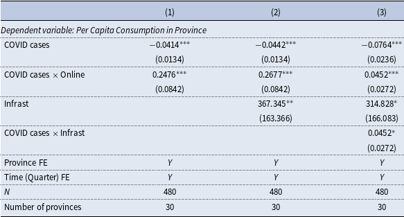
Table 1 displays the coefficient estimates. Consistent across specifications, we estimate a significant negative effect of the (proxy for) the intensity of the COVID shock on households’ per capita consumption (
 $\alpha \lt 0)$
. Most importantly for our analysis, the estimates reveal that this negative effect is significantly attenuated by a stronger development of the digital economy in the province (
 $\beta \gt 0$
). These conclusions remain virtually unaltered when we control for the provincial level of development of physical infrastructures.
Consumption, COVID, and the role of the online economy

Note: This table reports the estimates for the effects of the COVID shock and the development of the digital economy on consumption per capita in Chinese provinces. COVID cases is the number of cumulative infected COVID cases in the province. Online is the indicator for digital development of the province. Infrast is the proxy for physical infrastructures in the province, as given by the density of the road network. All regressions include province and time (quarter) fixed effects. ***,**,*. denote significance at the 1%, 5%, 10% level.
To summarize, the diff-in-diff analysis points to a material role of the online economy in attenuating the impact of the COVID shock on Chinese households’ consumption.
2.4 Further evidence from a SVAR analysis
To further investigate the stabilization role of online consumption during the COVID-19 pandemic, we next estimate a Structural Vector Autoregression (SVAR) model. The SVAR specification isFootnote 16
 \begin{equation} A_{0}Y_{t}=A_{1}Y_{t-1}+A_{2}Y_{t-2}+\epsilon _{t} \end{equation}
where the vector of endogenous variables,
 $Y_{t}=\left [ Lockdown_{t},OnlineCons_{t},TotalCons_{t}\right ]$
, includes a constructed lockdown index (see Section 3.2.5), and the HP-filtered log values of online and total consumption, all at weekly frequency. The sample runs from January 20 to September 28, 2020, with Pro-COVID trends based on 2019 data.
We identify the SVAR using a Cholesky decomposition, ordering the variables as in the vector
 $Y_{t}$
. This ordering assumes that lockdown shocks affect online and total consumption contemporaneously, and that online consumption can contemporaneously affect total consumption, but not vice versa.Footnote
17
Next, we also re-estimate the SVAR by replacing total consumption with offline consumption, defined as the deviation component of the HP-filtered log of offline retail consumption.Footnote
18
The impulse responses, displayed in Appendix Figure A.1, reveal key patterns that shed light on the dynamic interaction between lockdown measures and consumption behavior. A lockdown shock produces an immediate decline in all the three measures – online, total, and offline consumption (Panels (a), (b), and (d) in Appendix Figure A.1). However, the speed of recovery differs markedly. Online consumption rebounds the fastest, regaining its pre-COVID trend by around week 15. Total consumption follows more slowly, recovering by week 32, while offline consumption lags the most, returning to trend only by week 37. This staggered recovery pattern underscores the cushioning role of online consumption channels during periods of restricted mobility.
The responses to an online consumption shock further confirm its importance in sustaining aggregate demand. A one standard deviation increase in online consumption leads to a measurable and positive effect on both total and offline consumption (Panels (c) and (e)). The effect on total consumption is unsurprising, given the substantial share of online transactions in aggregate retail sales, but the positive effect on offline consumption suggests the presence of complementary demand spillovers – possibly reflecting households’ increased willingness to spend more broadly when digital channels function smoothly.Footnote 19
3. The model
In this section, we present our benchmark model before and after the outbreak of the epidemic. The model economy comprises households, firms, and the government. Households consume, save, and supply labor to firms. Firms produce goods by combining capital and labor. The government makes transfers (i.e., taxes when negative and subsidies when positive) during the epidemic.
3.1 The pre-infection economy
In this subsection we first present the household’s problem and then the firm’s problem. We assume that the steady state of the pre-infection economy is the starting point of the post-infection model economy.
3.1.1 The household’s problem
Prior to the epidemic, the economy is populated by a continuum of ex-ante identical households with measure one. In period
 $t$
, the representative household consumes offline consumption goods
 $\left ( c_{t}^{out}\right )$
and online consumption goods
 $\left ( c_{t}^{in}\right )$
, saves by purchasing firms’ shares
 $\left ( s_{t}\right )$
at price
 $q_{t}$
, and supplies labor
 $\left ( n_{t}\right )$
to firms. The representative household’s lifetime utility is given by (3)
 \begin{equation} \sum _{t=0}^{\infty }\beta ^{t}\left \{ \phi \ln c_{t}^{out}+\left ( 1-\phi \right ) \ln c_{t}^{in}-\frac {\theta }{2}n_{t}^{2}\right \} \end{equation}
where
 $\beta \in \left ( 0,1\right )$
denotes the discount factor, and
 $\phi$
and
 $\theta$
capture the utility weight of offline consumption and the disutility of labor, respectively.
The household’s period budget constraint is given by
 \begin{equation} c_{t}^{out}+p_{h}c_{t}^{in}+q_{t}s_{t}=w_{t}n_{t}+d_{t}s_{t-1}+q_{t}s_{t-1} \end{equation}
where
 $p_{h}$
denotes the price of e-commerce goods,
 $w_{t}$
denotes the real wage and
 $d_{t}$
denotes the dividends on the shares owned by the household that are distributed by firms. The household spends its labor income (
 $w_{t}n_{t}$
) and the revenues from holding period
 $t-1$
shares (
 $d_{t}s_{t-1}+q_{t}s_{t-1}$
) on offline and online consumption and for their purchase of period
 $t$
shares (
 $q_{t}s_{t}$
).
For simplicity, we normalize to one the price of offline consumption goods and treat the price of online consumption goods,
 $p_{h}$
, as a parameter. We assume that the price of online consumption goods is a fraction of that of offline consumption goods, that is,
 $p_{h}\lt 1$
. We calibrate the value of
 $p_{h}$
in Section 4 and provide arguments why
 $p_{h}\lt 1$
.
Let
 $\lambda _{bt}$
denote the Lagrangian multiplier associated with the budget constraint (4). The household’s problem is to choose offline and online consumption, savings, and labor supply to maximize its lifetime utility (3) subject to the budget constraint (4). The first-order conditions for the representative household’s problem are:
 \begin{align} \left [ c_{t}^{out}\right ] :& \quad \phi \frac {1}{c_{t}^{out}} =\lambda _{bt} \end{align}
 \begin{align} \left [ c_{t}^{in}\right ] :& \quad \left ( 1-\phi \right ) \frac {1}{c_{t}^{in}}=p_{h}\lambda _{bt} \end{align}
 \begin{align} \big[ n_{t}\big] :& \quad \theta n_{t}=\lambda _{bt}w_{t} \end{align}
 \begin{align} \big[ s_{t}\big] :& \quad q_{t}\lambda _{bt}=\beta \lambda _{bt+1}\big( d_{t+1}+q_{t+1}\big) \end{align}
3.1.2 The firm’s problem
There is a continuum of competitive representative firms of unit measure. The representative firm produces goods using capital (
 $k_{t}$
), labor (
 $n_{t}$
), and technology (
 $A_{t}$
) according to the Cobb-Douglas production function:
 \begin{equation} Y_{t}=A_{t}k_{t}^{\alpha }n_{t}^{1-\alpha } \end{equation}
For simplicity, we normalize
 $A_{t}$
to oneFootnote
20
We assume that the firm accumulates capital and that capital depreciates at the rate
 $\delta$
. The firm’s investment is given by
 \begin{equation} I_{t}=k_{t+1}-\big( 1-\delta \big) k_{t} \end{equation}
Define
 $d_{t}\equiv d\big( k_{t}\big) =k_{t}^{\alpha }n_{t}^{1-\alpha }-w_{t}n_{t}-\big( k_{t+1}-\big( 1-\delta \big) k_{t}\big)$
as the dividend paid by the firm to the household in period
 $t$
and
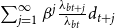
 $D\big( k_{t}\big) =\max \sum _{j=0}^{\infty }\beta ^{j}\frac {\lambda _{bt+j}}{\lambda _{bt}}d\big( k_{t+j}\big) =\max \sum _{j=0}^{\infty }\beta ^{j}\frac{u^{\prime }\big( c_{t+j}^{out}\big) }{u^{\prime }\big( c_{t}^{out}\big) }d\big( k_{t+j}\big)$
as the maximum value of the firm from period
 $t$
onwards.Footnote
21
The firm chooses capital (
 $k_{t+1}$
) and labor (
 $n_{t}$
) to maximize its value. We can write the firm’s problem in recursive form as
 \begin{equation} D\big( k_{t}\big) =\max _{\left \{ k_{t+1},n_{_{t}}\right \} }\left \{ k_{t}^{\alpha }n_{t}^{1-\alpha }-w_{t}n_{t}-\left ( k_{t+1}-\left ( 1-\delta \right ) k_{t}\right ) +\beta \frac {u^{\prime }\left ( c_{t+1}^{out}\right ) }{u^{\prime }\left ( c_{t}^{out}\right ) }D\left ( k_{t+1}\right ) \right \} \end{equation}
The first-order conditions for the firm’s problem read:
 \begin{align} \big[ n_{t}\big] :& \quad \left ( 1-\alpha \right ) \frac {Y_{t}}{n_{t}}=w_{t} \end{align}
 \begin{align} \big[k_{t+1}\big] :& \quad \beta \frac {u^{\prime }\big( c_{t+1}^{out}\big) }{u^{\prime }\big( c_{t}^{out}\big)}\big( \alpha \frac {Y_{t+1}}{k_{t+1}}+1-\delta \big) =1 \end{align}
In equilibrium, the representative household and the representative firm solve their optimization problems and the labor, goods, and asset markets clear.Footnote 22 Appendix F presents the solution for the steady state of the pre-infection economy, which serves as the initial point for the post-infection economy.
3.2 The outbreak of the epidemic
This subsection begins with some assumptions about testing and the households’ beliefs regarding their health status. We then proceed to detail the problems faced by the heterogeneous households and the representative firm during the pandemic. Finally, we present the specification of the lockdown shocks.
3.2.1 Testing and households’ beliefs about their health status
Modeling the macroeconomic effect of testing is challenging because the timing of testing and its accuracy can generate huge heterogeneity in people’s beliefs about their health status, thus inducing great heterogeneity in people’s economic decisions. As in Eichenbaum et al. (Reference Eichenbaum, Rebelo and Trabandt2022), to mitigate these sources of heterogeneity, we make some assumptions. First, we divide the population into a testing pool and a non-testing pool. In each period, the government tests
 $\mu$
percent of the population that has not yet been tested, resulting in a growing number of individuals in the testing pool over time depending on the value of
 $\mu$
. Second, we posit that those in the testing pool are tested every period until they recover or die. This assumption ensures that a person’s current economic decisions are not affected by the timing of their entry into the testing pool, but rather by his/her current health status. Third, we assume that tests are accurate, allowing for the revelation of a person’s health status. This assumption reduces the degree of heterogeneity without fundamentally changing the basic results.
We assume that each group (people outside the testing pool or people inside the testing pool) consists of four sub-groups: susceptible, infected, recovered, and deceased. The fraction of the susceptible, infected, recovered, and deceased people who are outside the testing pool are denoted by
 $S_{t}^{u},I_{t}^{u},R_{t}^{u}$
, and
 $D_{t}^{u}$
, respectively. The fraction of the susceptible, infected, recovered, and deceased people who are inside the testing pool are denoted by
 $S_{t}^{k},I_{t}^{k},R_{t}^{k}$
, and
 $D_{t}^{k}$
, respectively. At time zero, a fraction
 $\varepsilon$
of the population becomes infected. We assume that this information is public and that testing starts in period zero, so the initial conditions for the different groups of people are
 $I_{0}^{u}=\varepsilon,S_{0}^{u}=1-\varepsilon,R_{0}^{u}=0,I_{0}^{k}=S_{0}^{k}=R_{0}^{k}=0.$
Households’ beliefs about their health status. After period zero, individuals’ health status may change due to recovery or death for those infected and the possibility of infection for those susceptible. Individuals outside of the testing pool lack knowledge of their own health status and so form subjective probabilities regarding their health.
We denote individuals’ subjective probabilities regarding their health status at time
 $t$
, given they are alive at time
 $t$
(
 $a_{t}$
), as
 $p(s_{t}|a_{t})$
,
 $p(i_{t}|a_{t})$
, and
 $p(r_{t}|a_{t})$
for susceptibility
 $\left ( s_{t}\right )$
, infection
 $\left ( i_{t}\right )$
, and recovery
 $\left ( r_{t}\right )$
, respectively. It is assumed that in every period, a fraction
 $\pi _{r}$
of infected people recover and a fraction
 $\pi _{d}$
of infected people die. The subjective probability for susceptible individuals outside of the testing pool of becoming infected by the virus is denoted as
 $\tau _{t}^{u}$
. Appendix D details that the subjective probabilities of individuals becoming susceptible, infected, or recovered at time
 $t+1$
, conditional on being alive at time
 $t$
, are given by equations (14), (15), and (16), respectively.
 \begin{equation} p(s_{t+1}\mid a_{t+1}) [ 1-\pi _{d}p ( i_{t}\mid a_{t})] =( 1-\tau _{t}^{u}) p( s_{t}\mid a_{t}) \end{equation}
 \begin{equation} p\left ( i_{t+1}\mid a_{t+1}\right ) \left [ 1-\pi _{d}p\left ( i_{t}\mid a_{t}\right ) \right ] =\tau _{t}^{u}\,\,p\left ( s_{t}\mid a_{t}\right ) +\left ( 1-\pi _{r}-\pi _{d}\right ) p\left ( i_{t}\mid a_{t}\right ) \end{equation}
 \begin{equation} p\left ( r_{t+1}\mid a_{t+1}\right ) \left [ 1-\pi _{d}p\left ( i_{t}\mid a_{t}\right ) \right ] =p\left ( r_{t}\mid a_{t}\right ) +\pi _{r}p\left ( i_{t}\mid a_{t}\right ) \end{equation}
where
 $[ 1-\pi _{d}p( i_{t}\mid a_{t})]$
 $(\!=p( a_{t+1}\mid a_{t}))$
is the probability that the individual is still alive at time
 $t+1$
.
We assume that at time zero the probabilities that an individual outside the testing pool is susceptible, infected, or recovered are given by
 $p\left ( s_{0}\mid a_{0}\right ) =1-\varepsilon$
,
 $p\left ( i_{0}\mid a_{0}\right ) =\varepsilon$
,
 $p\left ( r_{0}\mid a_{0}\right ) =0$
, respectively. In the above equations, a key variable is
 $\tau _{t}^{u}$
, which represents the subjective probability of susceptible persons outside the testing pool that he or she is infected by the virus.Footnote
23
This variable plays a dual role as one of the determinants of both the subjective probabilities regarding individuals’ health states outside of the testing pool and the population dynamics across various groups of individuals. We will specify how
 $\tau _{t}^{u}$
is determined in the next subsection.
3.2.2 People outside the testing pool (or uncertain about health status)
The lifetime utility of an individual who is outside the testing pool at time
 $t$
,
 $U_{t}^{u}$
, is given by
 \begin{align} U_{t}^{u}=& u\big( c_{t}^{out,u},c_{t}^{in,u},n_{t}^{u}\big) +\left ( 1-\mu \right ) \beta \left [ 1-{\pi _{d}}p\left ( i_{t}\mid a_{t}\right ) \right ] U_{t+1}^{u} \notag \\ & +\mu \beta \left [ 1-\pi _{d}\left ( i_{t}\mid a_{t}\right ) \right ] \left [ p\left ( s_{t+1}\mid a_{t}\right ) U_{t+1}^{s}+p\left ( i_{t+1}\mid a_{t}\right ) U_{t+1}^{i}+p\left ( r_{t+1}\mid a_{t}\right ) U_{t+1}^{r}\right ] \end{align}
Here, the variables
 $U_{t+1}^{s},U_{t+1}^{i}$
, and
 $U_{t+1}^{r}$
denote the lifetime utility of a tested person who is susceptible, infected, and recovered at time
 $t+1$
, respectively. The parameter
 $\mu$
represents the fraction of people that enter the test pool (or the fraction of people who are certain about their health status). Equation (17) states that the lifetime utility of the person at time
 $t$
is equal to the current period utility
 $u( c_{t}^{out,u},c_{t}^{in,u},n_{t}^{u})$
plus the discounted expected lifetime utility from time
 $t+1$
. In period
 $t+1$
, the probability of an individual being alive and not in the testing pool is
 $\left ( 1-\mu \right ) \left [ 1-\pi _{d}\left ( i_{t}\mid a_{t}\right ) \right ]$
. The probabilities of an individual being alive and tested negative, positive, or recovered are given by
 $\mu \left [ 1-\pi _{d}\left ( i_{t}\mid a_{t}\right ) \right ] p\left ( s_{t+1}\mid a_{t}\right )$
,
 $\mu \left [ 1-\pi _{d}\left ( i_{t}\mid a_{t}\right ) \right ] p\left ( i_{t+1}\mid a_{t}\right )$
, and
 $\mu \left [ 1-\pi _{d}\left ( i_{t}\mid a_{t}\right ) \right ] p\left ( r_{t+1}\mid a_{t}\right )$
, respectively. The discounted expected lifetime utility from time
 $t+1$
is given by the sum of the second and the third terms in equation (17).
We assume that the period utility of the person outside the testing pool is given by
 \begin{equation} u\left ( c_{t}^{out,u},c_{t}^{in,u},n_{t}^{u}\right ) =\left ( 1-L_{t}\right ) \phi \ln c_{t}^{out,u}+\left ( 1-\chi L_{t}\right ) \left ( 1-\phi \right ) \ln c_{t}^{in,u}-\frac {\theta }{2}\left ( n_{t}^{u}\right ) ^{2} \end{equation}
where
 $c_{t}^{out,u}$
and
 $c_{t}^{in,u}$
denote the individual’s offline consumption and online consumption, respectively. The variable
 $0\lt L_{t}\lt 1$
represents lockdown shocks which reduce the utilities and, hence, demands for offline and online consumption. The parameter
 $0\lt \chi \lt 1$
captures the fact that lockdown shocks have relatively smaller effects on online consumption. In addition, we assume
 $n_{t}^{u}=\left ( 1-L_{t}\right ) n_{t}^{u}+L_{t}n_{t}^{u}$
. That is,
 $\left ( 1-L_{t}\right )$
fraction of labor is performed on-site and the remaining
 $L_{t}$
fraction of labor is performed at home.
We assume that lockdown shocks also directly affect online consumption through the presence in the utility function, for the following reason: although online consumption was more resilient than offline channels, it was not entirely insulated from lockdown-related disruptions. While certain segments of the online economy – particularly direct-distribution platforms such as JD.com, SF Express, and Hema Fresh – expanded rapidly by adopting models like “online ordering + contactless pickup lockers”, other parts of the online retail infrastructure experienced significant constraints. In particular, franchise-based delivery services (e.g., YTO, STO, and Yunda) saw substantial declines in volume – by as much as 35% or more – due to delayed resumptions of operations, cross-regional transportation bottlenecks caused by highway controls, and reduced efficiency at sorting hubs following tightened public health protocols. These operational frictions constrained consumers’ ability to access online goods and services during lockdowns.Footnote 24
The budget constraint of an individual outside the testing pool is given by
 \begin{equation} c_{t}^{out,u}+p_{h}c_{t}^{in,u}+q_{t}s_{t}^{u}=w_{t}n_{t}^{u}+d_{t}s_{t-1}^{u}+q_{t}s_{t-1}^{u}+\Gamma _{t}^{u} \end{equation}
where
 $s_{t}^{u}$
is the equity share held by an individual outside the testing pool, and
 $\Gamma _{t}^{u}$
is the lump-sum transfers. In steady state
 $\Gamma _{t}^{u}=0$
. For simplicity, following Zhao (Reference Zhao2020), we assume that the same wage rate
 $w_{t}$
is received by households, irrespective of their place of work.
In our model, the probability of being susceptible and infected at time
 $t+1$
for an individual outside the testing pool depends on
 $\tau _{t}^{u}$
, the probability of the susceptible person becoming infected at time
 $t$
, which in turn, depends on the social interactions between the susceptible and infected people outside the testing pool.Footnote
25
Following Eichenbaum et al. (Reference Eichenbaum, Rebelo, Trabandt and Koijen2021), we assume that social interactions occur in three ways: purchasing consumption goods, working, and engaging in non-economic activities. Thus, the probability that the virus is transmitted to a susceptible person outside the testing pool due to social interactions is given by
 \begin{eqnarray} \tau _{t}^{u}&=&\frac {1}{\sigma _{u}}\left [ \pi _{1}\left ( 1-L_{t}\right ) c_{t}^{out,u}\left ( 1-L_{t}\right ) I_{t}^{u}C_{t}^{out,u}\right.\nonumber\\&&\left. +\pi _{2}n_{t}^{u}\left ( 1-L_{t}\right ) I_{t}^{u}N_{t}\left ( 1-L_{t}\right ) +\pi _{3}\left ( 1-L_{t}\right ) I_{t}^{u}\left ( 1-L_{t}\right ) \right ] \end{eqnarray}
Here,
 $\left ( 1-L_{t}\right ) I_{t}^{u}C_{t}^{out,u}$
and
 $\left ( 1-L_{t}\right ) I_{t}^{u}N_{t}^{u}$
are the average consumption and hours worked of infected people, whose health status is unknown and who are subject to the lockdown restriction. In (20), the first two terms in the square brackets,
 $\pi _{1}\left ( 1-L_{t}\right ) c_{t}^{out,u}\left ( 1-L_{t}\right ) I_{t}^{u}C_{t}^{out,u}$
and
 $\pi _{2}n_{t}^{u}\left ( 1-L_{t}\right ) I_{t}^{u}N_{t}\left ( 1-L_{t}\right )$
, reflect virus transmissions that result from consumption- and work-related interactions, respectively. The parameter
 $\pi _{1}$
reflects the probability that the virus is transmitted as a result of shopping interactions. The parameter
 $\pi _{2}$
reflects the probability that the virus is transmitted as a result of work interactions. Note that in the first term, only people who do offline shopping interact with each other. Similarly, in the second term, only people who work on-site interact with each other. The term
 $\pi _{3}\left ( 1-L_{t}\right ) I_{t}^{u}\left ( 1-L_{t}\right )$
reflects transmissions that result from non-economic interactions, where
 $\pi _{3}$
reflects the probability that the virus is transmitted as a result of non-economic social interactions. Finally,
 $\sigma _{u}$
is a scaling parameter that is used to better match the health outcomes (e.g. the death rate and the infection rate).Footnote
26
The problem of an individual outside the testing pool is to maximize his or her lifetime utility (17) subject to the budget constraint (19), the transmission function (20), and the laws of motion for the probability of being susceptible (14) and infected (15).Footnote 27
The first-order conditions areFootnote 28
 \begin{align} \left [ c_{t}^{out,u}\right ] :& \quad \frac {\left ( 1-L_{t}\right ) \phi }{c_{t}^{out,u}}-\lambda _{bt}^{u}+\lambda _{\tau t}^{u}\frac {1}{\sigma _{u}}\pi _{1}\left ( 1-L_{t}\right ) ^{2}I_{t}^{u}C_{t}^{out,u}=0 \end{align}
 \begin{align} \left [ c_{t}^{in,u}\right ]:&\quad \frac {\left ( 1-\chi L_{t}\right ) \left ( 1-\phi \right ) }{c_{t}^{in,u}}-p_{h}\lambda _{bt}^{u}=0 \end{align}
 \begin{align} \left [ n_{t}^{u}\right ] :& \quad {-\theta n_{t}^{u}}+\lambda _{bt}^{u}w_{t}+\lambda _{\tau t}^{u}\frac {1}{\sigma _{u}}\pi _{2}\left ( 1-L_{t}\right ) I_{t}^{u}N_{t}^{u}\left ( 1-L_{t}\right ) =0\end{align}
 \begin{align} \left [ s_{t}^{u}\right ] :& \quad q_{t}\lambda _{bt}^{u}=\beta \lambda _{bt+1}^{u}\left [ 1-\pi _{d}p\left ( i_{t}\mid a_{t}\right ) \right ] \left ( d_{t+1}+q_{t+1}\right ) \\[10pt]\nonumber \end{align}
 \begin{equation} \left [ p\left ( i_{t+1}\mid a_{t+1}\right ) \right ] : \left ( \begin{array}{c} \frac {dU_{t}^{u}}{dp\left ( i_{t+1}\mid a_{t+1}\right ) }-\lambda _{it}^{u}\left [ 1-\pi _{d}p\left ( i_{t}\mid a_{t}\right ) \right ] +\beta \lambda _{it+1}^{u}p\left ( a_{t+1}\mid a_{t}\right ) \left ( 1-\pi _{r}-\pi _{d}\right ) \\[8pt] +\beta \lambda _{it+1}^{u}p\left ( a_{t+1}\mid a_{t}\right ) \pi _{d}p\left ( i_{t+2}\mid a_{t+2}\right ) +\beta \lambda _{st+1}^{u}p\left ( a_{t+1}\mid a_{t}\right ) \pi _{d}p\left ( s_{t+2}\mid a_{t+2}\right ) \\[8pt] +\beta \lambda _{rt+1}^{u}p\left ( a_{t+1}\mid a_{t}\right ) \pi _{r}+\beta \lambda _{rt+1}^{u}p\left ( a_{t+1}\mid a_{t}\right ) \pi _{d}p\left ( r_{t+2}\mid a_{t+2}\right ) =0\end{array}\right ) \end{equation}
 \begin{equation} \left [ p\left ( s_{t+1}\mid a_{t+1}\right ) \right ] :\quad \left ( \begin{array}{c} \frac {dU_{t}^{u}}{dp\left ( s_{t+1}\mid a_{t+1}\right ) }-\lambda _{st}^{u}\left [ 1-\pi _{d}p\left ( i_{t}\mid a_{t}\right ) \right ] +\beta \lambda _{it+1}^{u}p\left ( a_{t+1}\mid a_{t}\right ) \tau _{t+1}^{u} \\[8pt] +\beta \lambda _{st+1}^{u}p\left ( a_{t+1}\mid a_{t}\right ) \left ( 1-\tau _{t+1}^{u}\right ) =0\end{array}\right ) \end{equation}
where
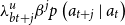 $\lambda _{bt+j}^{u}\beta ^{j}p\left ( a_{t+j}\mid a_{t}\right )$
,
 $\lambda _{\tau t+j}^{u}\beta ^{j}p\left ( a_{t+j}\mid a_{t}\right )$
,
 $\lambda _{st+j}^{u}\beta ^{j}p\left ( a_{t+j}\mid a_{t}\right )$
, and
 $\lambda _{it+j}^{u}\beta ^{j}p\left ( a_{t+j}\mid a_{t}\right )$
denote the Lagrange multipliers associated with the budget constraint (19), the transmission function (20), and the laws of motion for the probability of being susceptible (14) and infected (15), respectively.
3.2.3 People inside the testing pool
Under our assumptions about testing (Section 3.2.1), people inside the testing pool know whether they are susceptible, infected or recovered in the current period, but susceptible and infected people face uncertainty about their future health status.
Susceptible people Let
 $\tau _{t}^{s}$
be the probability that a susceptible person becomes infected and
 $1-\tau _{t}^{s}$
be the probability that a susceptible person remains susceptible. The lifetime utility of a susceptible person,
 $U_{t}^{s}$
, is
 \begin{equation} U_{t}^{s}=\left ( 1-L_{t}\right ) \phi \ln c_{t}^{out,s}+{\left ( 1-\chi L_{t}\right )} \left ( 1-\phi \right ) \ln c_{t}^{in,s}-\frac {\theta }{2}\left ( n_{t}^{s}\right ) ^{2}+\beta \left [ \left ( 1-\tau _{t}^{s}\right ) U_{t+1}^{s}+\tau _{t}^{s}U_{t+1}^{i}\right ] \end{equation}
where
 $c_{t}^{out,s}$
and
 $c_{t}^{in,s}$
denote the person’s offline consumption and online consumption, respectively. The person’s labor
 $n_{t}^{s}$
consists of work on-site,
 $\left ( 1-L_{t}\right ) n_{t}^{s}$
, and work at home,
 $L_{t}n_{t}^{s}$
.
The budget constraint is
 \begin{equation} c_{t}^{out,s}+p_{h}c_{t}^{in,s}+q_{t}s_{t}^{s}=w_{t}n_{t}^{s}+d_{t}s_{t-1}^{u}+q_{t}s_{t-1}^{u}+\Gamma _{t}^{s} \end{equation}
where
 $s_{t}^{s}$
is the equity share held by the susceptible person, and
 $\Gamma _{t}^{s}$
is the lump-sum transfers. In steady state
 $\Gamma _{t}^{s}=0$
.
The probability that the virus is transmitted to a susceptible person due to social interactions is given by
 \begin{eqnarray} \tau _{t}^{s}&=& \frac {1}{\sigma _{s}}\left[ \pi _{1}\left ( 1-L_{t}\right ) c_{t}^{out,s}\left( 1-L_{t}\right) I_{t}^{u}C_{t}^{out,u}\right.\nonumber\\&&\left. +\pi _{2}n_{t}^{s}\left ( 1-L_{t}\right ) I_{t}^{u}N_{t}^{u}\left ( 1-L_{t}\right ) +\pi _{3}\left ( 1-L_{t}\right ) I_{t}^{u}\left ( 1-L_{t}\right ) \right ] \end{eqnarray}
Similar to equation (20), the three terms on the RHS of equation (29) represent the three channels through which the susceptible individual is infected by the virus: the consumption channel, the working channel, and the non-economic channel. Again,
 $\sigma _{s}$
is the scaling parameter which is used to better match the health outcomes.
The problem of a susceptible individual is to maximize his or her lifetime utility (27) subject to the budget constraint (28) and the transmission function (29). The first-order conditions are
 \begin{align} \left [ c_{t}^{out,s}\right ] :& \quad \frac {\left ( 1-L_{t}\right ) \phi }{c_{t}^{out,s}}-\lambda _{bt}^{s}+\lambda _{\tau t}^{s}\frac {1}{\sigma _{s}}\pi _{1}\left ( 1-L_{t}\right ) ^{2}I_{t}^{u}C_{t}^{out,u}=0 \end{align}
 \begin{align} \left [ c_{t}^{in,s}\right ] :& \quad \frac {\left ( 1-\chi L_{t}\right ) \left ( 1-\phi \right ) }{{c_{t}^{in,s}}}-p_{h}\lambda _{bt}^{s}=0 \end{align}
 \begin{align} \left [ n_{t}^{s}\right ] :& \quad -\theta n_{t}^{s}+\lambda _{bt}^{s}w_{t}+\lambda _{\tau t}^{s}\frac {1}{\sigma _{s}}\pi _{2}\left ( 1-L_{t}\right ) I_{t}^{u}N_{t}^{u}\left ( 1-L_{t}\right ) =0 \end{align}
 \begin{align} \left [ s_{t}^{s}\right ] :& \quad q_{t}\lambda _{bt}^{s}=\beta \lambda _{bt+1}^{s}( d_{t+1}+q_{t+1}) \end{align}
where
 $\lambda _{bt}^{s}$
and
 $\lambda _{\tau t}^{s}$
are the Lagrange multipliers associated with the budget constraint (28) and the transmission function (29), respectively.
Infected people In our benchmark model, the identified infected people are quarantined and their consumption is provided by the government. For simplicity, we assume that they can maintain their consumption at the steady-state level of the pre-infection economy. Therefore,
 $c_{t}^{out,i}=c^{out}$
,
 $c_{t}^{in,i}=c^{in}$
. Clearly, infected people cannot (or are not allowed to) work. Therefore,
 $n_{t}^{i}=0.$
Footnote
29
To facilitate our counterfactual analysis, below we also present the problem of the infected people in a general case. An infected person at time
 $t$
could become recovered with probability
 $\pi _{r}$
at time
 $t+1$
, or remain infected with probability
 $1-\pi _{r}-\pi _{d}$
. The lifetime utility of an infected person,
 $U_{t}^{i}$
, is
 \begin{equation} U_{t}^{i}=\left ( 1-L_{t}\right ) \phi \ln c_{t}^{out,i}+\left ( 1-\chi L_{t}\right ) \left ( 1-\phi \right ) \ln c_{t}^{in,i}-\frac {\theta }{2}\left ( n_{t}^{i}\right ) ^{2}+\beta \left [ \left ( 1-\pi _{r}-\pi _{d}\right ) U_{t+1}^{i}+\pi _{r}U_{t+1}^{r}\right ] \end{equation}
The budget constraint is
 \begin{equation} c_{t}^{out,i}+p_{h}c_{t}^{in,i}+{q_{t}}s_{t}^{i}=w_{t}n_{t}^{i}+d_{t}s_{t-1}^{i}+q_{t}s_{t-1}^{i}+\Gamma _{t}^{i} \end{equation}
where
 $s_{t}^{i}$
is the equity share held by the infected person, and
 $\Gamma _{t}^{i}$
is the lump-sum transfers. In steady state
 $\Gamma _{t}^{i}=0$
.
The problem of an infected person is to maximize his or her lifetime utility (34) subject to the budget constraint (35). The first-order conditions are
 \begin{equation} \left [ c_{t}^{out,i}\right ] :\quad \frac {\left ( 1-L_{t}\right ) \phi }{c_{t}^{out,i}}-\lambda _{bt}^{i}=0 \end{equation}
 \begin{equation} \left [ c_{t}^{in,i}\right ] :\quad \frac {\left ( 1-\chi L_{t}\right ) \left ( 1-\phi \right ) }{c_{t}^{in,i}}-p_{h}\lambda _{bt}^{i}=0 \end{equation}
 \begin{equation} \left [ n_{t}^{i}\right ] :\quad -\theta n_{t}^{i}+\lambda _{bt}^{i}w_{t}=0 \end{equation}
 \begin{equation} \left [ s_{t}^{i}\right ] :\quad q_{t}\lambda _{bt}^{i}=\beta \lambda _{bt+1}^{i}\left ( d_{t+1}+q_{t+1}\right ) \end{equation}
where
 $\lambda _{bt}^{i}$
is the Lagrangian multiplier associated with the budget constraint (35).
Recovered people We assume that a recovered individual will not become infected or susceptible in the future. The lifetime utility of a recovered person,
 $U_{t}^{r}$
, is
 \begin{equation} U_{t}^{r}=\left ( 1-L_{t}\right ) \phi \ln c_{t}^{out,r}+\left ( 1-\chi L_{t}\right ) \left ( 1-\phi \right ) \ln c_{t}^{in,r}-\frac {\theta }{2}\left ( n_{t}^{r}\right ) ^{2}+\beta U_{t+1}^{r} \end{equation}
The person’s budget constraint is
 \begin{equation} c_{t}^{out,r}+p_{h}c_{t}^{in,r}+q_{t}s_{t}^{r}=w_{t}n_{t}^{r}+d_{t}s_{t-1}^{r}+q_{t}s_{t-1}^{r}+\Gamma _{t}^{r} \end{equation}
where
 $s_{t}^{r}$
is the equity share, and
 $\Gamma _{t}^{r}$
is the lump-sum transfers. In steady state
 $\Gamma _{t}^{r}=0$
.
The problem of a recovered individual is to maximize his or her lifetime utility (40) subject to the budget constraint (41). The first-order conditions read:
 \begin{align} \left [ c_{t}^{out,r}\right ] :& \quad \frac {\left ( 1-L_{t}\right ) \phi }{c_{t}^{out,r}}-\lambda _{bt}^{r}=0 \end{align}
 \begin{align} \left [ c_{t}^{in,r}\right ] :& \quad \frac {\left ( 1-\chi L_{t}\right ) \left ( 1-\phi \right ) }{c_{t}^{in,r}}-p_{h}\lambda _{bt}^{r}=0 \end{align}
 \begin{align} \left [ n_{t}^{r}\right ] :& \quad -\theta n_{t}^{r}+\lambda _{bt}^{r}w_{t}=0 \end{align}
 \begin{align} \left [ s_{t}^{r}\right ] :& \quad q_{t}\lambda _{bt}^{r}=\beta \lambda _{bt+1}^{r}\left ( d_{t+1}+q_{t+1}\right ) \end{align}
where
 $\lambda _{bt}^{r}$
is the Lagrange multiplier associated with the budget constraint (41).
3.2.4 Firms
We follow Zhao (Reference Zhao2020) in modeling the firm’s production function. Specifically, we assume that during the pandemic a fraction
 $\left ( 1-L_{t}\right )$
of labor is on-site and the remaining fraction
 $L_{t}$
of labor is performed at home. The production function is given by
 \begin{equation} Y_{t} =k_{t}^{\alpha }\left [ \left ( 1-L_{t}\right ) n_{t}+{\Phi L_{t}}n_{t}\right ] ^{1-\alpha } \end{equation}
Here, the parameter
 $\Phi$
 $\left ( 0\lt \Phi \lt 1\right )$
measures the productivity of workers who work from home relative to workers who work on-site.Footnote
30
The firm’s problem is to choose labor and capital to maximize its lifetime dividends:
 \begin{equation} \max \left \{ k_{t}^{\alpha }\left [ \left ( 1-L_{t}\right ) n_{t}+\Phi \left ( L_{t}\right ) n_{t}\right ] ^{1-\alpha }-w_{t}n_{t}-\left ( k_{t+1}-\left ( 1-\delta \right ) k_{t}\right ) +\beta \frac{u^{\prime }( c_{t+1}^{out,r}) }{u^{\prime }( c_{t}^{out,r}) }D( k_{t+1}) \right \} \end{equation}
where
 $D\left ( k_{t}\right ) =\max \sum _{j=0}^{\infty }\beta ^{j}\frac {\lambda _{bt+j}^{r}}{\lambda _{bt}^{r}}d\left ( k_{t+j}\right ) =\max \sum _{j=0}^{\infty }\beta ^{j}\frac {u^{\prime }\left ( c_{t+j}^{out,r}\right ) }{u^{\prime }\left ( c_{t}^{out,r}\right ) }d\left ( k_{t+j}\right )$
Footnote
31
is the maximum value of the firm and
 $d( k_{t}) =k_{t}^{\alpha }\left [ \left ( 1-L_{t}\right ) n_{t}+\Phi L_{t}n_{t}\right ] ^{1-\alpha }-w_{t}n_{t}-( k_{t+1}-( 1-\delta) k_{t})$
is the dividend of the firm.
The first-order conditions are given by
 \begin{align} \left [ n_{t}\right ] :& \quad \left ( 1-\alpha \right ) \frac {Y_{t}}{n_{t}}=w_{t} \end{align}
 \begin{align} \left [ k_{t+1}\right ] :& \quad \beta \frac {u^{\prime }\left ( c_{t+1}^{out,r}\right ) }{u^{\prime }\left ( c_{t}^{out,r}\right ) }\left ( \alpha \frac {y_{t+1}}{k_{t+1}}+1-\delta \right ) =1 \end{align}
3.2.5 Modeling the lockdown shocks
We construct the exogenous lockdown variable,
 $L_{t}$
, based on the Baidu daily within-city travel intensity index (Baidu index for short). We follow three steps to construct
 $L_{t}$
. In the first step, we normalize the Baidu index on January 20, 2020, to be one and calculate the corresponding index from January 21, 2020 to April 8, 2020. We then calculate the difference between one and the above calculated index from January 20 to April 8. We call the result the daily preliminary lockdown index. In the second step, we calculate the weekly average of the daily preliminary lockdown index and denote it by
 $l_{t}^{w}$
. In the third step, we construct the lockdown variable
 $\left ( L_{t}\right )$
by calculating the cumulative average of the weekly lockdown index from week 1 to week 9 as follows:Footnote
32
 \begin{equation} L_{t} =\frac {1}{1+j}\sum _{t=1}^{j+1}l_{t}^{w} \qquad \textrm {j}=0,1,2,\ldots 8 \end{equation}
We use the cumulative average for two reasons. First, it captures the persistence or the memory feature of the lockdown shocks. Indeed, although the adoption and lifting of the lockdown policy may be sudden, the real and psychological impacts of this policy may be relatively long-lasting. Second, if we directly used the weekly preliminary lockdown index
 $\left ( l_{t}^{w}\right )$
as the lockdown variable, the model economy would recover fairly quickly in response to the epidemic, which is inconsistent with the data.
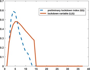
The preliminary lockdown index and lockdown shocks.

In Figure 2, the dashed curve shows the weekly preliminary lockdown index
 $\left ( l_{t}^{w}\right )$
, while the solid curve shows the lockdown variable
 $\left ( L_{t}\right )$
we use for our model. Compared to the weekly index, the peak of the lockdown variable occurred about one week later and it did not die out rapidly. Specifically, the lockdown variable increased sharply after the announcement of lockdown (January 23, 2020) and peaked between week 4 and week 5 (between February 17 and February 24, 2020). As the infection rate declined, the lockdown variable declined gradually. It turns out that this modeling of the lockdown variable can better capture the behavior of the key macroeconomic variables in response to the epidemic.
3.3 Population dynamics
The populations of people in different health states are important state variables in the model. The evolution of the size of susceptible, infected, recovered people, inside and outside the testing pool, and the evolution of the size of dead people, are given by equations (51)–(57), respectively. Appendix E contains the detailed explanations of these equations.
 \begin{equation} S_{t+1}^{k}=S_{t}^{k}-T_{t}^{k}+\mu \left ( S_{t}^{u}-T_{t}^{u}\right ) \end{equation}
 \begin{equation} S_{t+1}^{u}=\left ( 1-\mu \right ) \left ( S_{t}^{u}-T_{t}^{u}\right ) \end{equation}
 \begin{equation} I_{t+1}^{k}=T_{t}^{k}+\left ( 1-\pi _{r}-\pi _{d}\right ) I_{t}^{k}+\mu \left [ T_{t}^{u}+\left ( 1-\pi _{r}-\pi _{d}\right ) I_{t}^{u}\right ] \end{equation}
 \begin{equation} I_{t+1}^{u}=\left ( 1-\mu \right ) \left [ T_{t}^{u}+\left ( 1-\pi _{r}-\pi _{d}\right ) I_{t}^{u}\right ] \end{equation}
 \begin{equation} R_{t+1}^{k}=R_{t}^{k}+\pi _{r}I_{t}^{k}+\mu \left ( R_{t}^{u}+\pi _{r}I_{t}^{u}\right ) \end{equation}
 \begin{equation} R_{t+1}^{u}=\left ( 1-\mu \right ) \left ( R_{t}^{u}+\pi _{r}I_{t}^{u}\right ) \end{equation}
 \begin{equation} D_{t+1}=D_{t}+\pi _{d}\left ( I_{t}^{u}+I_{t}^{k}\right ) \end{equation}
3.4 Equilibrium
In equilibrium, agents solve their optimization problems and group-specific aggregates and individual levels of consumption and hours worked coincide:
 $c_{t}^{out,u}=C_{t}^{out,u}$
,
 $c_{t}^{in,u}=C_{t}^{in,u}$
,
 $c_{t}^{out,s}=C_{t}^{out,s}$
,
 $c_{t}^{in,s}=C_{t}^{in,s}$
,
 $c_{t}^{out,i}=C_{t}^{out,i}$
,
 $c_{t}^{in,i}=C_{t}^{in,i}$
,
 $c_{t}^{out,r}=C_{t}^{out,r}$
,
 $c_{t}^{in,r}=C_{t}^{in,r}$
,
 $n_{t}^{u}=N_{t}^{u}$
,
 $n_{t}^{s}=N_{t}^{s}$
,
 $n_{t}^{i}=N_{t}^{i}=0$
,
 $n_{t}^{r}=N_{t}^{r}$
.
The asset, goods, and the labor market equilibrium conditions and the government budget constraint are given by equations (58)–(61), respectively,Footnote 33
 \begin{equation} S_{t}^{k} s_{t}^{s}+I_{t}^{k} s_{t}^{i} +R_{t}^{k} s_{t}^{r} +\left ( S_{t}^{u}+I_{t}^{u}+R_{t}^{u}\right ) s_{t}^{u}=1 \end{equation}
 \begin{eqnarray}&&\qquad S_{t}^{k} \left(c_{t}^{out,s} + p_{h} c_{t}^{in,s} \right) + I_{t}^{k} \left(c_{t}^{out,i} + p_{h} c_{t}^{in,i} \right) + R_{t}^{k} \left(c_{t}^{out,r}+p_{h}c_{t}^{in,r}\right) \notag\\ &&\qquad\qquad + \left(S_{t}^{u} + I_{t}^{u} + R_{t}^{u}\right) \left(c_{t}^{out,u} + p_{h} c_{t}^{in,u} \right) + k_{t+1} - \left(1-\delta \right) k_{t} \notag \\&&\quad\qquad= k_{t}^{\alpha} \left[\left(1-L_{t}\right) N_{t}+\Phi L_{t}N_{t}\right]^{1-\alpha} \end{eqnarray}
 \begin{equation} N_{t}=S_{t}^{k}n_{t}^{s}+R_{t}^{k}n_{t}^{r}+\left ( S_{t}^{u}+I_{t}^{u}+R_{t}^{u}\right ) n_{t}^{u} \end{equation}
 \begin{equation} \Gamma _{t}^{i}I_{t}^{k}=\Gamma _{t}( S_{t}^{k}+R_{t}^{k}+S_{t}^{u}+I_{t}^{u}+R_{t}^{u}) \end{equation}
Equation (61) states that the government imposes lump-sum taxes
 $\left ( \Gamma _{t}\right )$
on susceptible
 $\left ( S_{t}^{k}\right )$
, recovered
 $\left ( R_{t}^{k}\right )$
and unknown health status people
 $\left ( S_{t}^{u}+I_{t}^{u}+R_{t}^{u}\right )$
to make transfers
 $\left ( \Gamma _{t}^{i}\right )$
to infected people
 $\left ( I_{t}^{k}\right )$
, where
 $\Gamma _{t}^{i}=c^{out}+p_{h}c^{in}$
.
4. Calibration
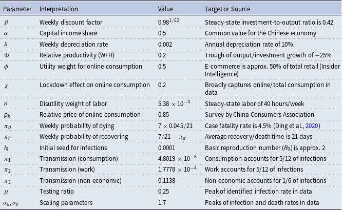
In our model, we set a unit of time as one week and proceed to calibrate the following parameters (see also Table 2). To begin, we specify the case fatality rate to be 4.5%, a figure corroborated by Ding, Cheng and Wan’s (2020) identification of the average COVID-19 case fatality rate in China up until March 18, 2020. Moreover, we assume that an individual infected with COVID-19 requires 21 days, on average, to either recover or die. For the purposes of a weekly model, we establish
 $\pi _{r}+\pi _{d}=7/21$
, wherein a 4.5% case fatality rate implies
 $\pi _{d}=7\times 0.045/21$
.
Calibrated parameters
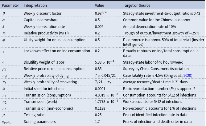
We follow the same assumptions outlined in Eichenbaum et al. (Reference Eichenbaum, Rebelo and Trabandt2022) to determine values of
 $\pi _{1}$
,
 $\pi _{2}$
, and
 $\pi _{3}$
. Specifically, we assume that the fraction of total infections associated with non-economic interactions at the beginning of the epidemic,
 $\left ( \pi _{3}I_{0}S_{0}\right )/ \left ( \pi _{1}S_{0}C^{2}I_{0}+\pi _{2}S_{0}N^{2}I_{0}+\pi _{3}I_{0}S_{0}\right )$
, is
 $1/6$
. Here,
 $S_{0}$
and
 $I_{0}$
are the total number of susceptible and infected people at the beginning of the epidemic, respectively, and
 $C$
and
 $N$
are consumption and hours worked in the pre-infection steady state. Furthermore, we posit that consumption and work-related activities each contribute equally to
 $(1-1/6)/2=5/12$
fraction of total infection at the beginning of the epidemic. That is,
 \begin{equation} \frac {\pi _{1}S_{0}C^{2}I_{0}}{\pi _{1}S_{0}C^{2}I_{0}+\pi _{2}S_{0}N^{2}I_{0}+\pi _{3}I_{0}S_{0}}=\frac {5}{12} \end{equation}
 \begin{equation} \frac {\pi _{2}S_{0}N^{2}I_{0}}{\pi _{1}S_{0}C^{2}I_{0}+\pi _{2}S_{0}N^{2}I_{0}+\pi _{3}I_{0}S_{0}}=\frac {5}{12} \end{equation}
In addition, we assume that without containment policies, as the standard SIR model indicates, eventually 83 percent of the population either recovers from the infection or dies.Footnote 34 That is,
 \begin{equation} R_{H}+D_{H} =0.83 \end{equation}
Here, the subscript
 $H$
denotes the time horizon by which
 $83\%$
of the population either recovers or dies. In the simulation, we choose
 $H=200$
, corresponding to nearly 4 years.
 $R_{H}$
and
 $D_{H}$
denote the recovery rate and the cumulative death rate at period
 $H$
, respectively.Footnote
35
Equations (62), (63) and (64) constitute a system of non-linear equations in
 $\pi _{1},\pi _{2}$
and
 $\pi _{3}$
. Solving this system numerically, we obtain that
 $\pi _{1}=4.8019\times 10^{-8},\pi _{2}=$
 $1.7778\times 10^{-4}$
and
 $\pi _{3}=$
 $0.1138$
. We set the initial seed of infection at
 $0.0001$
. This parameter, together with other parameters, implies that
 $R_{0}$
is about
 $2$
, which is consistent with the value of this parameter reported by Riou and Althaus (Reference Riou and Althaus2020).
We set the weekly depreciation rate,
 $\delta$
, at
 $0.002$
, implying an annual depreciation rate of
 $10\%$
. Moreover, we choose the capital share
 $\alpha$
to be 0.5, a commonly used value for the Chinese economy. Additionally, we specify the annual discount factor to take a value of
 $0.98$
. Thus, the weekly discount factor can be calculated as
 $\beta =0.98^{\frac {1}{52}}$
. Using these parameters, we evaluate the steady-state ratio of investment to output and find it to be approximately
 $0.42$
, in agreement with empirical observations. Furthermore, the relative productivity parameter, denoted by
 $\Phi$
, exerts a pivotal impact on the growth rates of output and investment. We set it to be
 $0.2$
, which manifests in a trough of roughly
 $-25$
percent for the growth rate of output and investment.
As outlined in Section 3.1.1, we normalize the price of offline consumption goods to be
 $1$
and posit that the price of online consumption goods
 $p_{h}$
is less than 1. In a survey paper on digital economics, Goldfarb and Tucker (Reference Goldfarb and Tucker2019) provide a clear explanation for why online consumption goods are typically priced lower than their offline counterparts. First, online transactions generally involve lower search costs, which enable consumers to easily locate and compare a broad range of prices for similar goods. A number of empirical studies confirm this argument, with Brynjolfsson and Smith (Reference Brynjolfsson and Smith2000) reporting substantially reduced prices for books and CDs when purchased online. Second, purchasing goods online allows for reduced transportation costs, particularly in situations where offline purchasing may be inconvenient, if not impossible. Pozzi (Reference Pozzi2013) illustrates that consumers capitalize on online shopping to specifically minimize transportation costs. Our calibration exercise is guided by a report by the China Consumers Association that indicates that the average price of online consumption goods was approximately
 $15\%$
less than offline consumption goods between December 2016 and March 2017. Thus, we parameterize
 $p_{h}$
at 0.85.
We set the parameter
 $\phi$
, which characterizes the demand for online consumption goods, to be
 $0.5$
. As reported by Insider Intelligence, e-commerce in China continues to eclipse traditional brick-and-mortar retail sales as a percentage of the total retail market, with the proportion leaping from
 $35\%$
in 2019 to
 $52.1\%$
in 2021. The value of
 $\chi$
is assigned to
 $0.2$
, implying a limited effect of lockdowns on online consumption. The value of
 $\theta$
, which characterizes the disutility weight of labor supply, is set at
 $5.38\times 10^{-4}$
, implying a steady state value of labor supply of
 $40$
hours per week.
In Eichenbaum et al. (Reference Eichenbaum, Rebelo and Trabandt2022), the assumption is made that the testing ratio, represented by
 $\mu$
in our model, is an exceedingly small number. This hypothesis aligns well with the low testing rates observed in various regions of the United States. For our model, we opt to set
 $\mu$
at
 $0.25$
, a higher value than the aforementioned assumption. There are several justifications for this choice. Firstly, a value of
 $\mu$
at 0.25 can more closely mirror the peak of the confirmed infection rate. Secondly, we adopt a broader interpretation of
 $\mu$
, interpreting it as the fraction of individuals with a clear understanding of their health status. As noted in Section 2 and Appendix A, China has employed numerous strategies such as large-scale random testing and targeted testing via contact tracing and health QR codes, which provide greater clarity regarding the health status of their citizens. For instance, community staff promptly contact individuals who have been detected to have come into contact with infected individuals, requiring them to undergo quarantine. Similarly, if someone has recently visited a high-risk area, their health QR code will reflect this information and they may be compelled to undergo testing and possibly quarantine. Through such a rigorous implementation of containment and public health policies, uncertainty regarding one’s health status is reduced. Thirdly, the chosen value of
 $\mu$
is not unrealistic in comparison with rates suggested in the literature. For example, Romer (Reference Romer2020) has suggested testing 7 percent of the US population on a daily basis, implying a weekly testing rate of 50 percent of the US population.
Finally, the scaling parameters
 $\sigma _{u}$
and
 $\sigma _{s}$
are set at
 $1.7$
to approximately match the peak of the infection rate and the cumulative death rate.
5. Results
In this section, we first present the health and macroeconomic outcomes predicted by our benchmark model and compare them with the data. We show that our model can capture some key characteristics of the data. Based on this, we then conduct several experiments to explore the influence of the online economy, the roles of the implementation and timing of the lockdown policy, and the role of testing. Our main results are that the online economy plays a fundamental role in reducing economic costs; ineffective lockdowns are associated with higher health costs and lower economic costs; prompt lockdown is associated with lower health costs; and testing plays an important role in reducing health costs.
5.1 Results of the benchmark model
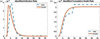
Figure 3 depicts the observed health outcomes (dashed line) alongside the predictions of our benchmark model (solid line). Specifically, Figure 3(a) presents the identified infection rate (
 $I^{k}$
), i.e., the proportion of identified infected individuals to the initial population. The data indicates that the peak of infection occurred in week 5. Our model predicts that the peak occurs between weeks 2 and 3. While our model forecasts the peak of infection earlier than the observed data, it nevertheless predicts well the magnitude of the peak.
Figure 3(b) displays the identified cumulative death rate (
 $D^{k}$
), which represents the percentage of the initial population that succumbs to the virus. The data reflects a sudden jump in deaths owing to adjustments made by Chinese authorities. Our model cannot fully replicate this discontinuity, only being capable of generating a smooth trajectory. However, it does manage to roughly track the general trajectory of cumulative deaths observed in the data. Overall, our model can broadly replicate crucial data of the epidemic.
Health outcomes in the data and in the benchmark model (a) First outcome. (b) Second outcome.

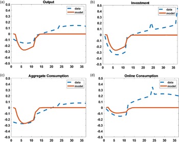
Macroeconomic variables in the data and in the benchmark model.

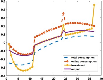
Figure 4 compares the percentage deviations from steady state for several key macroeconomic variables. The dashed blue lines represent the percentage deviations of output, investment, total consumption, and online consumption from their respective steady states in the data. We define each variable’s steady state as its average weekly value in 2019, consistent with the model’s assumption that the pre-pandemic state reflects the steady state.Footnote 36 The solid red lines show the corresponding percentage deviations generated by our benchmark model. Our analysis focuses on the first 15 weeks – spanning January 20 to April 27, 2020 – because the economy had largely recovered by week 16. Since the model is designed to converge to a steady state, it is not intended to capture the post-recovery fluctuations in the data.
While the model does not perfectly replicate the observed dynamics over this period, it successfully captures several key features of China’s macroeconomic trajectory. First, it replicates the U-shaped pattern of the percentage deviations. Second, it closely matches the timing of the troughs. For instance, in the data, output reaches its trough in week 6 (March 2, 2020), while the model predicts the trough in week 5 (February 24, 2020). The trough in total consumption occurs in week 5 in both the data and the model, while investment reaches its trough in week 4 in the data and week 5 in the model.
Finally, the model broadly captures the timing of macroeconomic recovery. In the data, the deviation of output from its steady state turns positive in week 14 (April 27, 2020); in the model, output reaches its steady state in the same week. Similarly, investment returns to its steady state in week 15 (May 4, 2020) in both the data and the model. Total consumption, however, recovers later in the data. It turns positive in week 33 (September 7, 2020), whereas the model shows recovery by week 15. Online consumption recovers earlier: in the data, its deviation becomes positive in week 11 (April 6, 2020), while in the model it reaches its steady state by week 15.
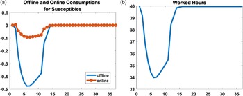
Figure 5 presents additional predictions generated by our benchmark model. Figure 5(a) displays the projected deviations of offline and online consumption from their respective steady states for susceptible individuals.Footnote 37 The model predicts that the decline in offline consumption is approximately five times larger than that in online consumption. Figure 5(b) shows the predicted dynamics of worked hours (i.e., equilibrium average employment). The steady state level of worked hours is 40; however, during the pandemic, this figure declined rapidly, reaching a trough of 34 in week 6.
The model-based predictions of consumption and worked hours.

5.2 Applications
5.2.1 More on the role of the online economy
To assess the impact of the online economy on the COVID-19-induced economic downturn, we conduct a counterfactual analysis by setting the parameters
 $\phi =0.999$
and
 $\Phi =0$
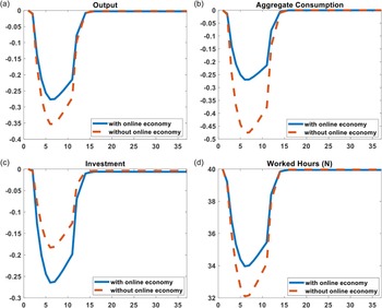
. This specification implies that most consumption occurs offline and that individuals do not engage in remote work due to zero productivity in that channel. Figure 6 presents the simulation results. The solid blue lines represent percentage deviations from steady state in the benchmark model with an online economy, while the dashed red lines represent the model without the online economy.
Our findings indicate that the online economy plays a significant role in mitigating the recession. In Figure 6(a), the absence of the online economy results in a much deeper and more prolonged output decline. Although both models reach their trough in week 5, output falls by about 8 percentage points more in the model without the online economy. The online economy also has a large effect on total consumption.Footnote 38 As shown in Figure 6(b), the deviation of total consumption from its steady state is substantially greater and more persistent without the online economy. While both models reach their consumption troughs in week 5, the drop in the model without the online economy is approximately 21% deeper than in the benchmark model.
Figure 6(c) shows the results for investment, which may initially seem counterintuitive: investment falls less in the model without the online economy. This is due to the model’s structure. Since
 $\Phi$
and
 $\phi$
affect output and consumption differently, the model without the online economy generates a smaller decline in output relative to consumption. To restore equilibrium in the goods market, investment must rise relative to its baseline. While this behavior is not central to our model’s intended contribution, the results for output and consumption remain realistic.
Figure 6(d) shows the evolution of hours worked. Without the online economy, hours decline substantially more, indicating that remote work plays a meaningful role in preserving labor input during the pandemic.
Macroeconomic variables in the benchmark model and the model without the online economy.

Our model suggests that the online economy has limited impact on health outcomes. The total infection rate and death rate are nearly identical in both scenarios. On the one hand, the presence of the online economy reduces interpersonal contact, thus lowering infection risk. On the other hand, in the absence of the online economy, lower consumption and reduced hours worked also decrease exposure, offsetting any gains from digital adaptation. This reflects the modeling assumption that the transmission rates (
 $\tau _{u}$
and
 $\tau _{s}$
) are proportional to consumption and labor effort.
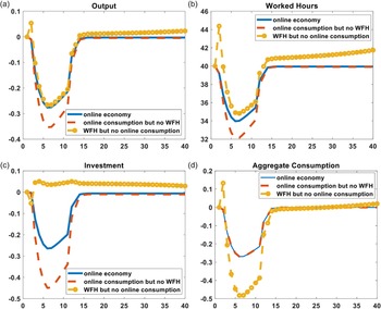
To further examine the contributions of the two main components of the online economy – online consumption and working from home (WFH) – we conduct two sets of quantitative experiments.
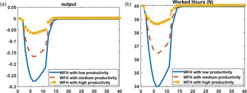
Disentangling online consumption and remote work In the first experiment, we compare macroeconomic outcomes (deviations of output, hours worked, investment, and total consumption) across three scenarios: (i) the benchmark model with both online consumption and WFH; (ii) a model with online consumption only; and (iii) a model with WFH only.
Figure 7 presents the simulation results across the three scenarios, where the solid blue lines represent scenario (i), the dashed red lines represent scenario (ii), and the dashed yellow lines with circles represent scenario (iii). Several key insights emerge from this comparison. First, working from home (WFH) plays a critical role in stabilizing output during the pandemic. In scenario (ii), where WFH is absent, output falls by 35% at the trough. In contrast, when WFH is included – as in scenarios (i) and (iii) – the decline in output is more moderate, reaching only 27%. This suggests that the ability to work remotely helped maintain productive capacity despite severe restrictions on mobility. Second, WFH also mitigates employment losses. In scenario (ii), hours worked fall to 32 hours per week at the trough, compared to 34 hours in scenario (i). However, the inclusion of online consumption alone, as in scenario (ii), does not substantially affect labor market outcomes, indicating that remote work is the more critical channel for preserving employment levels (scenario iii). Third, WFH plays an important role in buffering the decline in investment. In scenario (ii), investment contracts by 45% at the trough, while in the full model (scenario (i)), the drop is much smaller – only 27%. Counterintuitively, investment actually rises in scenario (iii), where WFH is excluded but online consumption is present. This counterintuitive result reflects underlying equilibrium adjustments in the goods market, which we discuss further in the footnote.Footnote 39 Finally, online consumption is found to be essential for stabilizing aggregate consumption. In scenario (iii), where online consumption is excluded, total consumption drops sharply – by as much as 48% at the trough. In contrast, scenarios (i) and (ii), both of which include online consumption, show a significantly milder contraction in total consumption, limited to around 27%. This highlights the crucial role that online consumption played in sustaining household demand during the most restrictive phases of the pandemic.
Macroeconomic dynamics under different types of online economy.

To summarize, WFH is especially important for mitigating declines in output, employment, and investment, while online consumption plays a central role in sustaining aggregate demand. These findings are particularly relevant to China, where rapid advances in e-commerce and remote work technologies enabled households and firms to adapt flexibly under strict lockdowns. Our model’s distinction between online and offline channels, as well as the inclusion of WFH, offers a nuanced understanding of how China’s digital infrastructure helped cushion the economic impact of the pandemic.
Productivity of remote work In the second experiment, we assess how WFH productivity affects macroeconomic outcomes by varying the productivity parameter
 $\Phi$
from 0.2 (benchmark) to 0.5 and 0.8. Since varying the productivity parameter has limited impact on aggregate consumption and generates noisy investment results, we focus on output and hours worked. Figure 8(a) shows that improving WFH productivity significantly reduces output losses. When
 $\Phi$
increases from 0.2 to 0.5 and then to 0.8, output contraction at the trough drops from 27% to 16% and then to just 6%. Figure 8(b) shows a similar pattern in hours worked: trough levels improve from 34 to 36 and 38 hours per week, respectively.
These findings underscore the importance of digital infrastructure and remote work capabilities as macroeconomic stabilizers. From a policy perspective, strengthening the online economy – especially by enhancing WFH productivity – can play a vital role in minimizing the adverse economic effects of future epidemic outbreaks.
Output growth and hours worked under different levels of WFH productivity.

5.2.2 The role of the effectiveness of lockdown
In the absence of vaccines and effective treatments during the early phase of the COVID-19 pandemic, nationwide lockdowns – though extreme – became a common and urgent response adopted by many countries. However, the success of a lockdown policy depends not only on its adoption but also, critically, on how effectively it is implemented. Following the literature, including Alvarez et al. (Reference Alvarez, Argente and Lippi2021) and Goenka et al. (Reference Goenka and Liu2024), we introduce a parameter
 $\rho \in (0,1]$
to capture the variations in lockdown enforcement. Specifically, all lockdown-related terms in the model are scaled by
 $\rho$
, where
 $\rho =1$
denotes full effectiveness, and lower values indicate reduced implementation quality.
In our benchmark model, we assume
 $\rho =1$
, reflecting effective lockdown implementation. This assumption is supported by Feng et al. (Reference Feng, Wu, Yuan and Zhou2022), who construct a measure of pandemic containment effectiveness (PCE) across 100 countries between January 3 and November 27, 2020. Using a stochastic cost frontier approach, they assess PCE based on mortality data while accounting for underreporting. During the first two weeks after the first reported death (January 11, 2020 for China), China ranked near the bottom among 10 major economies due to the virus’s early and rapid spread. However, China’s PCE ranking improved significantly over time due to swift government response, large-scale resource mobilization, and strict containment policies. By late June, China ranked 21st out of 97 countries, indicating effective virus control. Since lockdown was one of the most critical containment tools, we regard
 $\rho =1$
as a reasonable representation of China’s experience during the first wave.
To examine the consequences of less effective policy implementation, we simulate outcomes under
 $\rho =1$
,
 $\rho =0.8$
, and
 $\rho =0.75$
. Figure 9 presents the health outcomes – specifically, the aggregate infection rate (
 $I^{k}+I^{u}$
) and the cumulative death rate (
 $D^{k}+D^{u}$
). Several findings emerge: First, infection rates increase substantially as
 $\rho$
declines, indicating that poor enforcement leads to wider viral spread (Figure 9(a)). Second, when
 $\rho =1$
, infections peak in week 2 and decline smoothly to zero by week 15. When
 $\rho \lt 1$
, however, the infection rate initially declines but later resurges, indicating a failure to sustain containment. Third, cumulative death rates are substantially higher under less effective lockdowns (Figure 9(b)). With
 $\rho =1$
, deaths plateau after week 17, but with
 $\rho =0.75$
, fatalities continue to rise throughout the simulation window.
Figure 10 displays the corresponding economic outcomes. Weaker enforcement (i.e., lower values of
 $\rho$
) is associated with smaller short-run economic losses: output, investment, total consumption, and online consumption all decline less sharply when lockdowns are less strictly implemented. This highlights a classic policy trade-off: stronger lockdowns reduce infections and deaths more effectively but impose greater short-term economic costs.
Our model thus underscores that lockdown effectiveness plays a pivotal role in shaping both health and economic outcomes. While stricter and well-implemented lockdowns come with sharper near-term economic losses, they deliver better public health results and support a more stable recovery trajectory. These results are consistent with our broader interpretation that effective implementation capacity – an institutional and social feature – should be viewed as a key dimension of societal resilience. We revisit this point in Section 5.2.5.
Total infected and total deaths predicted by models with 100%, 80%, 70% of lockdowns.

Macroeconomic variables predicted by models with 100%, 80%, 70% of lockdowns.

5.2.3 The effects of the timing of lockdown
We next examine the impact of lockdown timing on pandemic outcomes. In this experiment, we assume that the government delays implementing the lockdown policy by two weeks. Specifically, the lockdown in our model begins in week 3 instead of week 1. Figure 11 presents the health outcomes under this delayed scenario. Both the total infection rate and the cumulative death rate are noticeably higher when the lockdown implementation is delayed. Figure 12 displays the economic outcomes, which show that the decline in output and total consumption is postponed correspondingly.
This experiment underscores the critical importance of timely lockdown implementation. A prompt response can substantially reduce health costs without amplifying economic losses. As the leading official of Wuhan City remarked in a CCTV (China Central Television) interview during the early 2020 outbreak, had the lockdown decision been made earlier, the situation in Wuhan would have been more favorable, and the epidemic’s spread to other regions might have been mitigated. Nonetheless, in early 2020, the epidemic’s nature and scale remained highly uncertain, and implementing such an extreme policy in a major metropolis was a difficult and unprecedented decision.
Infection rate and death rate with lockdown in week 1 (solid lines) and lockdown in week 3 (dashed lines).

Output and aggregate consumption with lockdown in week 1 (solid lines) and lockdown in week 3 (dashed lines).

5.2.4 The role of testing
To evaluate the role of testing, we conduct a counterfactual experiment by setting the testing rate parameter,
 $\mu$
, to 0.01 – a very low value. Our findings show that drastically reducing the testing rate, while keeping lockdown measures in place, has limited effects on economic outcomes. Since the macroeconomic variables under
 $\mu =0.01$
are nearly indistinguishable from those in the benchmark model, we do not display them in figures. Intuitively, when lockdowns are enforced, individuals’ uncertainty about their health status has little additional impact on aggregate macroeconomic behavior. Accordingly, our model attributes the observed contraction and recovery of output, investment, and consumption primarily to the imposition and removal of lockdown policies.
However, the health outcomes are substantially worse when testing is minimal, as shown in Figures 13(a)–(f). These panels illustrate the dynamics of the identified infection rate (
 $I^{k}$
), unidentified infection rate (
 $I^{u}$
), total infection rate (
 $I^{k}+I^{u}$
), identified death rate (
 $D^{k}$
), unidentified death rate (
 $D^{u}$
), and total cumulative death rate (
 $D^{k}+D^{u}$
). Several findings stand out. First,
 $I^{k}$
and
 $D^{k}$
are markedly lower under a low testing rate, which is expected. Second, with a high testing rate (
 $\mu =0.25$
),
 $I^{k}$
spikes and then declines rapidly. By contrast, when testing is low,
 $I^{k}$
persists and even resurges (Figure 13(a)). Similarly, with high testing,
 $D^{k}$
peaks in week 18 and remains stable thereafter. Under low testing,
 $D^{k}$
stays lower but steadily increases without bound (Figure 13(b)). Third, low testing leads to higher and more persistent values for
 $I^{u}$
,
 $D^{u}$
,
 $I^{k}+I^{u}$
(total infections) and
 $D^{k}+D^{u}$
(total deaths).
These patterns are consistent with the model’s structure. Equation (54) shows that the unidentified infection rate (
 $I_{t+1}^{u}$
) declines with higher testing rate (
 $\mu$
). Equations (20) and (29) indicate that infection probabilities rise with
 $I_{t}^{u}$
through non-economic interactions. Thereafter, even under lockdown, if testing is inadequate, unidentified carriers may continue spreading the virus, keeping total infections and deaths high. Our results highlight that widespread testing and isolation of infected individuals are critical to minimizing the health costs of a pandemic.
Infected and deaths in the benchmark model and the model with very low testing.

5.2.5 Discussion: Societal resilience and the online economy
While the preceding subsections have examined the health and economic outcomes under different policy scenarios, this subsection reflects on two broader insights from our analysis.
First, we highlight the importance of societal resilience – a country’s ability to absorb, adapt to, and recover from large-scale shocks while maintaining essential functions (Brunnermeier, Reference Brunnermeier2021). Although resilience is inherently multidimensional and difficult to capture fully in a formal model, our framework approximates it through two key mechanisms: the strength of the online economy and the effectiveness of lockdown implementation.
The rapid expansion of China’s digital infrastructure prior to the pandemic – ranging from e-commerce and digital payments to remote work capabilities – enabled households and firms to adapt quickly to mobility restrictions. As our simulations show, online consumption helped stabilize aggregate demand, and work-from-home mitigated employment losses and investment declines. In this sense, digital channels provided both continuity and flexibility, softening the economic blow of the lockdowns. This is consistent with international findings such as those by the OECD (2021), which identifies digital readiness as a key pillar of macroeconomic resilience in the face of pandemics.
In addition, the effectiveness of China’s containment efforts – driven by swift and well-coordinated policy execution, logistical capacity, and public compliance – also reflected institutional resilience. Our model captures this through enforcement quality, showing that stronger lockdowns reduce infection rates and death tolls more effectively, albeit at greater short-term economic cost.
Second, our findings support the view that restoring public confidence in virus containment is critical for economic recovery (Chetty et al., Reference Chetty, Friedman, Hendren and Stepner2020; Romer, Reference Romer2020; Feng et al. Reference Feng, Wu, Yuan and Zhou2022). Virus transmission involves significant externalities, meaning that private decisions alone cannot effectively limit spread. Government interventions – such as lockdowns, mass testing, and isolation of infected individuals – are necessary to contain outbreaks and reduce uncertainty. In the case of China, the rapid and stringent implementation of such measures not only suppressed infections but also signaled control, helping to reassure the public and enabling a faster recovery in consumption and output. These dynamics reinforce the argument that economic normalization depends on successful pandemic containment.
6. Conclusion
This paper utilizes a SIR-macro model to analyze the health and economic consequences of the first wave of the COVID-19 epidemic in China. Our analysis highlights the importance of two key structural features – the online economy and containment policies – in mitigating the pandemic’s health and economic toll. On May 5, 2023, the World Health Organization declared that COVID-19 no longer constituted a public health emergency of international concern. While the world has entered the post-pandemic era, new and unpredictable shocks remain inevitable. Some may resemble the pandemic in magnitude and systemic disruption. It is therefore crucial to draw lessons from past responses to improve preparedness and resilience. As our analysis suggests, societies that are better equipped to respond – through technological readiness, effective governance, and adaptive capacity – may bend under the weight of crisis, but they need not break.
Supplementary material
The supplementary material for this article can be found at http://doi.org/10.1017/S1365100525100722.
Acknowledgements
We are grateful to the editor, an associate editor and two anonymous referees for their comments. For helpful comments and conversations, we also thank Martin Eichenbaum, S. Nuri Erbas, Bo Li, Minghao Li, Jin Song, Zheng (Michael) Song, Shu Xu, Bo Zhao, Xiaodong Zhu and seminar and conference participants at Asia Meeting of the Econometric Society, East and Southeast Asia (Singapore), Asia Meeting of the Econometric Society in China (Shenzhen, virtual), Australasia Meeting of the Econometric Society (Brisbane, virtual), CCER Summer Institute (Beijing), China Economic Annual Conference (Guangzhou), Annual Meeting of Economic Fluctuation and Growth Research Workshop (Xiamen), Michigan State University, Royal Economic Society Annual Conference (Glasgow). We thank Zheng (Michael) Song for providing us with within-city travel data. Ying Tung Chan acknowledges the financial support from National Natural Science Foundation of China (NSFC) Grant No. 72203022.