The process of economic growth is rarely uniform: as an economy gets richer, so its structure also changes. In Argentina, much of the national economic debate over the twentieth century has concerned the causes and desirability of structural change, as the country industrialized and the traditionally dominant agricultural sector declined in relative importance. This article formalizes one strand of this long-standing debate in an attempt to answer the following question: what was the underlying cause of structural change in Argentina after the end of the Belle Epoque through the period of import-substituting industrialization (ISI)? The two obvious candidates are the policies of ISI themselves, and the decline in the land-labor ratio that occurred over the same period. Such a question can only be answered in a general equilibrium framework, which we provide in the form of a stylized CGE model.
The rise of manufacturing has exercised Argentine economists at least since Alejandro E. Bunge's (Reference Bunge1920) discussion of the implications of the closing of the land frontier. Bunge argued that the high wages produced by the rural sector made manufacturing uncompetitive, and that high import tariffs were therefore required to protect it. But the formulation of trade policy inevitably involves conflict between exporting and import-competing sectors of the economy, making the question of industrial protection highly political. As Guillermo O'Donnell (Reference O'Donnell1978) has famously argued, in Argentina the pendular swing of power between these groups fed back to economic outcomes in the form of the stop-go economy. Indeed, the conflict over trade policy continues to the present day, as demonstrations by the rural sector and its supporters against a rise in export taxes shook the Argentine government in mid-2008.
In his classic analysis of the Argentine economy, Carlos Díaz-Alejandro (Reference Díaz-Alejandro1970) argued that the trade policies of ISI, by reducing the relative price of agricultural goods,Footnote 1 deterred production and investment in that sector. He states that “during 1945–1955, domestic policies depressed the outlook for rural activities producing exportables” (p. 206). This is a standard view of the impact of ISI: its effect on relative prices benefitted import-competing manufacturing at the expense of exporting agriculture.
In contrast to Díaz Alejandro, and following Bunge (Reference Bunge1920), Guido Di Tella (Reference Di Tella and Brodersohn1970) emphasizes the importance of the closing of the land frontier in the process of industrialization. Di Tella argues that “the growth of the population exceeded the ‘growth’ of the stock of exploited land, and therefore the possibility of excess labor appeared… the employment capacity of industry was considered one of its main justifications from the beginning of its development” (p. 440).
These different perspectives imply two alternative explanations for structural change in Argentina. The ISI explanation is that policies that biased relative prices in favor of industry and against agriculture caused a slowdown and relative decline in agriculture. The factor endowments explanation is that it was caused by the decline in the land-labor ratio, due to land being in limited supply after a certain point while the population and hence labor force continued to grow.
The two explanations in turn imply different historical counterfactuals. We first test the ISI explanation econometrically by estimating price elasticities of sectoral output in the data. Our time-series regressions do not support the view that price changes had a significant impact on agricultural output. The core of the article, however, is an analysis of the different counterfactuals using a calibrated dynamic three-sector, three-factor computable general equilibrium (CGE) model. We construct a SAM for 1935 based on a combination of data for 1935 (the first year with current-price national accounts data and only the second year of full employment since 1929) and Argentina's first input-output matrix from 1950, running the model to 1960 (see Appendix 2 for a discussion of data and sources). The model has two tradable sectors, agriculture which is exported and industry which is import-competing, in addition to a third non-tradable services sector.
Such a simple model cannot hope to capture the rich detail of a real economy over 25 years, but with calibration it replicates the key sectoral trends. It also maps on to historical policy discussions, and is simple enough that the outcomes can be understood intuitively. But the presence of a third, non-tradable sector takes the model beyond the historical debate, where policy decisions are often represented as a zero-sum game between industry and agriculture. Since non-tradable services comprise approximately half of value added in our period of interest, the inclusion of this third sector makes a significant difference to the analysis.
Our approach is in the spirit of Allen C. Kelley and Jeffrey G. Williamson's (Reference Kelley and Williamson1973) two-sector analysis of Japan over 1887–1915, in which counterfactuals are simulated to establish the importance of different factors in explaining growth and structural change. Similarly, Alan M. Taylor (Reference Taylor1995) produces a CGE for Argentina for the period 1870–1914 in order to analyze the effect of immigration on wages and output. Here we simulate the following four counterfactuals. First, trade and other policies that affect the domestic relative price of tradables are fixed at their pre-ISI 1929 level, so that changes in domestic prices are driven primarily by changes in international prices. Second, the tariff is removed altogether. In the third simulation, the domestic relative price of industry to agriculture stays constant at its 1935 level, as if both trade policy and international prices were staying constant. These simulations indicate the role of relative prices in determining output, and hence the importance of ISI in determining the evolution of the structure of the economy.
In the final simulation, the area of available arable land continues to grow at the rate of labor supply growth after 1935, keeping the land-labor ratio constant rather than declining as in the data. The difference between this simulation and the baseline simulation tells us how important the closing of the land frontier was in determining the structure of the economy. In terms of standard trade theory, this is conceptually similar to estimating the Rybczinski effect of changing factor endowments,Footnote 2 where relative factor intensities in different sectors drive structural change.
In addition to policy- and factor endowment-induced changes in economic structure, structural change can also be induced by changes in relative demand. Cristina Echevarria (Reference Echevarria1997), Piyabha Kongsamut, Sergio Rebelo, and Danyang Xie (Reference Kongsamut, Rebelo and Xie2001), and Jürgen Meckl (Reference Meckl2002) model structural change as the result of non-homothetic preferences, and Engel's Law in particular, according to which people spend a declining share of their incomes on food (and hence agricultural produce) as their incomes rise. In this spirit, we model demand using a linear expenditure system, where demand for each sector's output has a subsistence level that must be satisfied, with remaining income distributed in fixed proportions. Since agriculture and industry are tradable this has no impact on their relative price, but in general equilibrium does have an impact on the relative price of non-tradables.Footnote 3
While the present article addresses relative growth rates of different sectors within the Argentine economy, a further debate exists over the causes of Argentina's general decline over the twentieth century relative to the leading economies. Di Tella and D. C. H. Platt (Reference Di Tella and Platt1986) argue that Argentina's slow growth after the closing of the land frontier was due to its failure to move from a rent-based economy to an economy based on “industry of the Schumpeterian kind, continuously introducing new technologies, new products, and new cost-reducing procedures” (Di Tella and Platt Reference Di Tella and Platt1986, p. 124). Díaz Alejandro (Reference Díaz-Alejandro1970) argues that poorly designed tariff structures led to high relative prices of capital goods, lowering real investment. On the other hand, Taylor (Reference Taylor1992) argues that investment was constrained by a low supply of savings, itself caused by a high dependency ratio. These arguments help to explain low productivity growth in the economy as a whole, but do not explain the different rates of growth observed across sectors, which is the focus of this study.
A study of the Argentine economy that addresses both aggregate growth and the controversial question of agricultural decline is Yair Mundlak, Domingo Cavallo, and Roberto Domenech (Reference Mundlak, Cavallo and Domenech1989). They model the longer period of 1913–1984 and also use a three-sector model. Unlike the present analysis, they divide the economy into agriculture, non-agriculture, and government. Among their findings is that alternative policies could have led to increased growth in the economy, including much higher output in the agricultural sector. However, they assume that the supply of land available for cultivation could have grown without limit, and this assumption is necessary for their finding that more favorable policies towards agriculture could have had a large impact on aggregate growth.Footnote 4 We find this assumption implausible. The consistent data series of total cultivated land extends to 1984, covering the dramatic rise in agricultural and other commodity prices in 1974 and the radical opening of the economy implemented by the dictatorship of 1976–1983 in which the trade policies of ISI were reversed. Despite these changes, the area of cultivated land never substantially exceeded the peak reached in 1934.Footnote 5 Thus the reaching of the arable frontier does appear to have placed a binding constraint on the amount of cultivated land, at least within plausible bounds on the price of agriculture, contradicting the assumption of Mundlak, Cavallo, and Domenech.
ECONOMIC DEVELOPMENT AND STRUCTURAL CHANGE IN ARGENTINA, 1900–1960
Argentina first grew rich during the Belle Epoque, from the late nineteenth century to the beginning of the First World War. It had developed a reputation as a great exporting nation, despite average import tariffs consistently above 20 percent, and by 1913 was the tenth richest economy in the world in per capita terms (Coatsworth and Williamson Reference Coatsworth and Williamson2004; Maddison Reference Maddison2010). Over 2 million immigrants, the majority from Italy and Spain, had travelled across the Atlantic to find a better standard of living.Footnote 6 Growth was interrupted by the First World War, which caused substantial economic decline as both export markets and the importation of key intermediate goods were disrupted. The economy returned to growth immediately after the war, but in per capita terms real GDP did not return to its 1913 level until the mid-1930s, after recovering from the Great Depression (Cortés Conde Reference Cortés Conde1997, pp. 18–19).
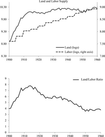
Of particular importance for the analysis we present below, the Great Depression coincided with the closing of the land frontier. Land use had grown very rapidly before the First World War, with the total area of cultivated land tripling over 1900–1913. By 1913 Argentina's whole stock of high quality arable land was within reach of the railroad (Cortés Conde Reference Cortés Conde1979, p. 177–78), but landowners had not taken full advantage of this access until twenty years later. The year 1934 was both the year in which the area of cultivated land stopped growing, and in which total GDP returned to its 1929 level at full employment. As pointed out by Bunge (Reference Bunge1920), labor supply continued to rise as the availability of arable land did not: Figure 1 plots the area of cultivated land and the total labor supply in the economy and, in the second panel, the land-labor ratio. Until 1913 the growth of land was much more rapid than that of labor, but the land-labor ratio then began a long secular decline.
Population growth was particularly high during the Belle Epoque, much of it due to European immigrants attracted by the high wages that they could earn.Footnote 7 James R. Scobie (Reference Scobie1964, pp. 60–61) writes that for a migrant worker from Italy or Spain, “four to five months’ labor in the wheat-corn harvest could bring from forty to fifty pounds sterling—five to ten times what he could earn in his homeland,” while Roberto Cortés Conde (Reference Cortés Conde1979, p. 265) estimates that real wages in Argentina at the beginning of the twentieth century were about double those in Italy. As a result, over 1895–1914 immigration's contribution to population growth was 17.2 per thousand (Cortés Conde Reference Cortés Conde, Cárdenas, Antonio Ocampo and Thorpe2000, pp. 276–78). Moreover, Cortés Conde finds that the level of immigration rose and fell over time with the level of wages in Argentina.
During the Great Depression, however, immigration collapsed, to a total of only 4,400 over the three years 1932–1934. Immigration from Europe picked up again in the years following the Second World War, though this was driven by political as much as economic factors. Estimates presented by Gino Germani (Reference Germani1966) indicate that net immigration over 1901–1930 was equivalent to 31 percent of total population growth, dropping to 11 percent of total population growth over 1941–1960. The percentage of the population of Argentina that was foreign-born declined monotonically from a high of 29.9 percent in 1914 to 23.5 percent in 1930, 15.8 percent in 1950, and 12.8 percent in 1960.Footnote 8 The early 1930s is known as the point of transition to the import-substitution era. While tariffs during the Belle Epoque were relatively high, and close to their 1930s average, they declined below 20 percent during the First World War, remaining low through the 1920s (Coatsworth and Williamson Reference Coatsworth and Williamson2004).Footnote 9 The improvised attempts to shore up the balance of payments during the Great Depression in the early 1930s, including exchange controls in 1931, devaluation in 1933, and an increase in import tariffs in 1932, led almost accidentally to industrial protection (Katz and Kosacoff Reference Katz, Kosacoff, Cárdenas, Antonio Ocampo and Thorpe2000). The main author of the policy response to the Great Depression, Raúl Prebisch, has stated that he and his team of economists believed that industry needed to be promoted in order to reduce imports. But the official purpose at this stage was to address the balance of payments deficit, not to promote industry for its own sake or to promote national self-sufficiency per se. Moreover, he reported, “all public opinion was against industrialization,” so “high customs duties were imposed without stating that their purpose was to encourage industrialization; the group of young men who were behind these steps were very careful not to make any reference to industrialization” (Prebisch Reference Prebisch, Di Tella and Platt1986, p. 134). It was later that these measures became part of an explicit strategy of import-substituting industrialization, also involving import quotas, differential exchange rates, and subsidized credit for industry. Some reordering of the industrial strategy was attempted in the 1960s, but the basic economic approach did not change radically until the military government of the late 1970s, which dramatically opened the economy.Footnote 10 Our end point of 1960 is thus at the tail end of the ISI period.
SUPPLY OF LAND (MILLIONS OF HECTARES) AND LABOR (MILLIONS OF WORKERS)

Data on output by sector, at 1950 prices, are available from 1900. We divide the economy into agriculture (including livestock), industry (including both mining, and processed agricultural goods such as tobacco, “foods and drinks,” and leather), and non-traded services. Simply plotting these data illustrates that the key change in economic structure that took place in Argentina over 1900–1960 was the relative decline in agriculture and the rise of manufacturing, in terms of both output and employment. Figure 2 shows log output and employment in the three sectors, where employment estimates are five-year averages up to 1947. Output growth in agriculture was lower than in manufacturing and services throughout the period, but there is a marked slowdown in the sector in the second half of the period.Footnote 11 Turning to employment, labor force growth in agriculture slowed and almost stopped in the mid-1930s, and indeed reversed in the early 1950s. Hence on both these measures the picture is of relative decline in the agricultural sector after the 1930s.
SECTORAL OUTPUT AND EMPLOYMENT, LOGS

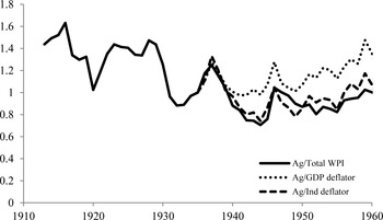
RELATIVE PRICES OF THE AGRICULTURAL SECTOR, WPI AND GDP DEFLATOR, 1935 = 1

IMPORT-SUBSTITUTING INDUSTRIALIZATION AND RELATIVE PRICES
The introduction of policies to protect the balance of payments in the early 1930s, and the later deepening of ISI proper, are generally perceived to have worsened the internal terms of trade for the agricultural sector. Figure 3 shows three relative price series, all indexed to 1 in 1935. The series starting in 1913 is the wholesale price of agricultural goods divided by the wholesale price index of the “whole economy.” Up to 1925 the nonagricultural component of the latter is based on prices of a small set of manufactured goods only and the composition after that time is unclear (see Appendix 2), suggesting that one should use the index with caution. But it does seem to imply that relative agricultural prices so measured were substantially lower after 1930 than before, aside from a partial recovery in the late 1930s. The 1937 local peak is higher than any subsequent year in the period.
The two series starting in 1935 are agriculture's price deflator divided respectively by the GDP deflator and industry's price deflator, calculated using current price data at factor prices, and output indices, from national accounts. Unfortunately, data on GDP at current prices are available only from 1935 so this series cannot be extended further back in time. The series relative to the price of industry is much closer to the WPI, supporting the interpretation that the non-agriculture component of the WPI for the “whole economy” may really be measuring prices of industrial output and not accounting properly for services, unlike the GDP deflator.
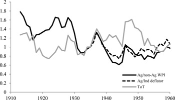
DOMESTIC RELATIVE PRICES AND THE TERMS OF TRADE, 1935 = 1

Relative prices of tradeables are determined, of course, not just by domestic policy but also by international prices. The large majority of Argentina's exports were agricultural products while most imports were manufactures and this suggests a comparison between the terms of trade and these domestic relative prices. Again, this comparison should be treated with caution: manufactures comprised between 51 and 64 percent of the value of imports over 1950–1960, with most of the remainder comprising fuels and other crude materials. Agriculture's share of exports was higher at about 90 percent.Footnote 12
Bearing in mind these qualifications, Figure 4 gives the WPI for agriculture relative to non-agriculture, the GDP deflator for agriculture relative to manufacturing, and the international terms of trade (i.e., the international price of exports relative to imports), all indexed to 1935 = 1. When the terms of trade are higher than the domestic relative price indices in the figure, it means that the relative international price of agriculture is higher than the relative domestic price compared with 1935, such as would occur under an increased tariff on imported manufactures relative to the 1935 baseline.
Considering the WPI series, compared with 1935, the relative domestic price of agricultural products is generally higher than the terms of trade before 1930, and lower from about the late 1930s (recalling that they are equal by construction in 1935), supporting the view that domestic policies were more supportive of industry relative to agriculture after 1935 than before. We now turn to the question of whether these prices actually affected output.
RELATIVE PRICES AND OUTPUT IN THE DATA
While policies may have been unfavorable to the agricultural sector, there is no evidence in the data that prices had an impact on output in that sector. Díaz Alejandro (Reference Díaz-Alejandro1970, p. 169) regresses agricultural output on prices using yearly data over 1929–1965 and finds no significant relationship. When we regress log agricultural output on its log relative wholesale price over the longer period 1913 to 1960, there is a strong negative correlation. However, both series appear to be nonstationary, with Augmented Dickey-Fuller test statistics outside the 10 percent critical value. The residuals appear to be stationary (at 5 percent but not 1 percent significance) so the two series are I(1), and Engle-Granger tests suggest that they are cointegrated. We therefore run an error correction modelFootnote 13 with the following results:
 \begin{equation}
\Delta InY_A = 0.015 - \begin{array}{*{20}c}
{0.266L\xi } \\
{\left({0.090} \right)} \\
\end{array} - \begin{array}{*{20}c}
{0.030\Delta \ln p_A } \\
{\left({0.14} \right)} \\
\end{array},\,\,N = 47
\end{equation}
where YA is output in agriculture, PA is the WPI price of agriculture divided by the WPI index for the whole economy, ζ is the residual from a regression of YA on PA , L is the lag operator, and Δ the difference operator. Standard errors are in parentheses. The coefficient on the lagged residual ζ indicates a statistically significant attraction to equilibrium, but the coefficient on the change in price is not close to being significant. We ran further ECMs with up to four lags, with and without time trends, and in no case was ΔinpA or any of its lags significant.
The lack of a relationship with the price is indicated more clearly by the equivalent autoregressive distributed lag (ADL) model. Using one lag, as assumed in the ECM above, we find the following:
 \begin{equation}
{*{20}c}
{\Delta InY_A = 0.015 - } \hfill & {0.266L\xi - } \hfill & {\,\,0.030\Delta \ln p_A,} \hfill & {\,\,\,\,\,\,N = 47} \hfill \\
{} \hfill & {\left({0.090} \right)} \hfill & {(0.14)} \hfill & {} \hfill \\
\end{equation}
With the lagged dependent variable as a control, the coefficients on the relative price and its lag are not significantly different from zero, and are of the wrong sign. Again we ran similar regressions with between zero and four lags in each of the dependent variable and the relative price, with and without time trends, and in none of them was the price or any of its lags ever close to significant.
Turning to the industrial sector, we do find limited evidence of a positive price elasticity of output. Again, we cannot reject the null that log output is nonstationary, according to a Dickey-Fuller test. Its first differences do appear to be stationary so we assume it is I(1). As we saw above, the wholesale price index of “non-agriculture” starts off using only industrial goods, and then follows the industrial GDP deflator closely. So we use this price divided by the WPI index for the whole economy as an indicator of the price of industry. We can reject the null that this series is nonstationary at approximately the 1 percent level.Footnote 14 We therefore regress the first difference of log output on the price level and find that the price is insignificant, as follows:
 \begin{equation}
{InY_A = 2.43 + } \hfill & {0.734LinY_A } \hfill & { - \,\,0.027\ln p_A } \hfill & { - \,\,0.181Linp_A \,\,\,\,\,N = 47} \hfill \\
{} \hfill & {\left({0.09} \right)} \hfill & {(0.15)} \hfill & {\,\,\,\,\,\left({0.15} \right)} \hfill \\
\end{equation}
where standard errors are again in parentheses. However, running an ADL for the first difference of output on price we find that the lagged price does have a significantly positive effect:
 \begin{equation}
{*{20}c}
{\Delta InY_1 = 0.04 - } \hfill & {0.044inP_{I,} } \hfill & {N = 47} \hfill & {\,\,\,\,\,} \hfill \\
{} \hfill & {\left({0.11} \right)} \hfill & {} \hfill & {} \hfill \\
\end{equation}
Here the positive coefficient on the lagged price is significant at the 5 percent level while the other regressors are all insignificant. Adding further lags renders all the price variables insignificant.
We do not have a plausible price index for services before 1935 (since the “non-agriculture” WPI is primarily industry) so we cannot do an equivalent analysis for this sector. The 26-year period 1935–1960 for which we have the GDP deflator is too short for plausible results.
To summarize, there is some evidence that output in industry positively responds to its own relative price, but no evidence of this for agriculture. Absence of evidence is, of course, very different from evidence of absence: these results are probably the result of weaknesses in the data, rather than positive support for a zero price elasticity of output in agriculture. The number of data points is relatively low, policies and the economic environment changed during the period in ways that cannot be captured in the data, and these are aggregated sectors. Rather, the lack of plausible results from these regressions indicates that a purely empirical approach is not adequate to analyze the changes we observe over the period. Moreover, such regressions are necessarily partial equilibrium results. For these reasons, a full analysis requires a CGE model which will capture the economic mechanisms at work, including the interactions between the sectors.
THE MODEL
We now present a dynamic CGE model of the economy which we then use to construct counterfactuals to explore the underlying causes of structural change. Here we describe the outline of the model, while Appendix 1 provides the details and explains the calibration. The theoretical starting point is a standard three-sector, three-factor competitive model, such as those described in W. M. Corden and J. P. Neary (Reference Corden and Neary1982), which we implement as a simplified and highly stylized version of the dynamic CGE of Clemens Breisinger, Xinshen Diao, and James Thurlow (Reference Breisinger, Diao and Thurlow2009).Footnote 15
The three productive sectors are agriculture, industry, and services, as used in the empirical analysis above. Production functions are CES in factors of production, where agriculture uses land, labor, and capital, while industry and services use only labor and capital. Agriculture is exported and its domestic price is equal to its international price. Industry is import-competing, where consumers demand an Armington composite of imports and domestic production. This implies that, in a standard analysis where international prices of tradables are taken as exogenous, industry prices faced by consumers and producers are nonetheless endogenous. Services are not traded so their price is also endogenous. Preferences of the representative household are modeled using a linear expenditure system (LES) over agriculture, composite industry, and services.
The supply of labor is endogenously determined as the amount of employment in the data plus a variable component that depends on the relative wage. This accounts for international immigration. The area of land cultivated is endogenous but, following our earlier discussion of the land frontier, the supply is constrained by the highest recorded quantity of land cultivated, which was achieved in 1968, outside our period of analysis.Footnote 16 The capital stock is endogenized by assuming a savings rate, and that net investment equals saving minus depreciation.Footnote 17 Capital is putty-clay where the share of new investment going to each sector is rising in the return to capital in that sector, implying limited capital mobility. That is, a higher return to capital in a given sector leads to a higher share of investment being directed to that sector, but not all new investment goes to the sector with the highest return. We further assume a lag of one year between the investment allocation decision and the appearance of the new capital.Footnote 18
The main additional complication that we add relative to Breisinger, Diao, and Thurlow is that labor mobility is also restricted in our model, with a fixed share of labor in each sector assumed to be mobile each period. Like capital investment, the proportion of all mobile labor that moves to each sector is rising in the returns to labor in that sector. We restrict labor mobility partly because it is realistic and partly because in our calibrations we found that a fully mobile labor force led to large swings in production that are not found in the data. We saw above that we cannot find a significant elasticity of output with respect to price in the data for the agricultural sector. But we do not wish to close down the response to prices altogether, so limited factor mobility provides a theoretically plausible compromise.
In calibrating the baseline model, we treat the domestic price of both tradable sectors as exogenous, using the sectoral GDP deflators in the data. In the case of industry, this is the price faced by producers. From the point of view of the economy, the producer price of industry is endogenous, determined by international prices and the rest of the model. But it is changes in this producer price that are suspected to have had an impact on economic structure, partly due to the policies of ISI, so from the point of view of our calibration we need to ensure that this price follows the data. We therefore allow the international price of industry to be endogenous in the baseline model. We then change this assumption when we produce the counterfactual simulations with no ISI, as discussed below.
COUNTERFACTUALS: PRICES, FACTOR ENDOWMENTS, AND STRUCTURAL CHANGE
We are interested in changes in the structure of the economy due to both changes in relative prices and changes in relative factor endowments. Relative prices evolve following changes in both international prices and trade policy, while the most important change in factor endowments, as we have seen, is the rise of labor and capital relative to land. It is these variables that we change in our counterfactual simulations.
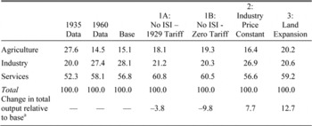
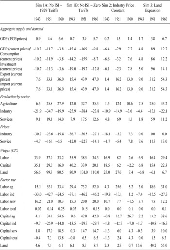
Table 1 reports the share of total value added in each of the three sectors in 1935 and 1960 in the data and in different model simulations, and the impact on total GDP. Details on the values taken by further variables of interest can be found in Appendix Table 3. The first column of Table 1 presents sector shares in 1935, which are common to the data and all simulations. The second column presents the data in 1960, and the third column the 1960 shares in the baseline simulation which was used to calibrate the model, and is intended to produce output by sector as close to the data as possible. Total output is less than 1 percent different from the data, and all shares are within one percentage point of the shares in the data.
The remaining columns present 1960 sector shares in four different simulations representing four different counterfactuals. The first two simulations, 1A and 1B, are different versions of a “no ISI” scenario in which we cut the tariff rate for the years 1936–1960. Agriculture is the numeraire and we make the evolution of the international price of industry exogenous, following the external terms of trade data, allowing the domestic producer price of industry to vary endogenously. Domestic prices therefore follow the evolution of international prices, mediated by the constant reduced tariff rate and the Armington assumption of the model. Hence the rising tariffs and all other distortions that were implied by ISI are absent in these simulations.
In simulation 1A, we set tariffs equal to their pre-crisis 1929 level of 17.3 percent for the years 1936 to 1960, lowered from the 1935 value of 23.1 percent (Díaz Alejandro Reference Díaz-Alejandro1970, p. 282). This is below the tariff level of the high-growth and export-driven period of the Belle Epoque: over 1880–1914 tariff revenue was consistently over 20 percent of the value of imports (Coatsworth and Williamson Reference Coatsworth and Williamson2004). While average official tariffs were around 20 percent through the 1920s, tariff revenue as a share of the cost of imports dropped below 20 percent from around the beginning of the First World War (Díaz Alejandro Reference Díaz-Alejandro1970, p. 280–85). This occurred in Argentina, as in many other countries, because standard practice was to set tariffs as a share of official prices of imports, not of actual prices. Inflation during the First World War raised the cost of imports without increasing tariff revenue, leading to tariff revenue briefly falling below 10 percent of import values over 1918–1921. It then rose again during the 1920s with postwar deflation (Coatsworth and Williamson Reference Coatsworth and Williamson2004, p. 227). The value of 17.3 percent attained in 1929, just before the Great Depression and the implementation of the policies associated with ISI, seems a plausible counterfactual representing relatively free trade.
In simulation 1B, we set tariffs equal to zero. This counterfactual is suggestive of truly free trade, but we consider it to be a theoretical possibility rather than a plausible alternative that the government could have pursued. John Coatsworth and Williamson (Reference Coatsworth and Williamson2004, p. 216) point out that “customs revenues are especially important for land-abundant countries with federal governments since low population and taxpayer density make other forms of tax collection inefficient.” The government had little realistic alternative to import tariffs as a source of revenue.
Turning to the results, we compare output in each sector under the counterfactual simulations with that in the baseline simulation. In simulation 1A, agriculture is 3 percentage points higher in 1960, industry 6.9 lower, and services 4 higher. This implies that the deepening of ISI over the period almost fully accounts for the 7.4 percentage point rise in industry's share over the period. But the cost to agriculture's share was relatively modest, with most of the reduction in output share coming from services instead. In simulation 1B, as expected, the results are in the same direction as simulation 1A but slightly larger for both agriculture and industry. Relative to the baseline simulation, agriculture is 4.2 percentage points higher in 1960, industry 7.9 lower, and services 3.7 higher.
In simulation 2, the relative producer price of domestic industry to agriculture is kept constant at its 1935 level. This therefore represents a counterfactual in which there is no change in either policy or international prices over the period. Relative to the base simulation, agriculture gains 1.4 percentage points, industry loses 1.2, and services gain 0.1. This implies that the impact of the changes in domestic prices over the period 1935 to 1960 was relatively modest.
Simulation 3 is the same as the baseline except that we keep the land-labor ratio constant by allowing the available stock of land to grow at the same rate as the labor supply. Now agriculture gains 5.2 percentage points relative to the base simulation, industry loses 7.6, and services gain 2.4.
Table 1 also reports the change in total output in each of the simulations. It may be surprising that the “no ISI” simulations lower total GDP by 3.8 percent with 1929 tariffs and by 9.8 percent with zero tariff over the period: in a perfectly competitive and frictionless economy one would expect a reduction in a tariff to increase GDP. Two mechanisms explain this. First, higher TFP growth in industry implies that a higher output share of industry leads to higher aggregate growth. Second, the presumption that reducing the tariff increases output disappears when one accounts for the kinds of frictions that we model here. In particular, limited factor mobility implies that changes over time in relative prices are costly, because they imply an inefficient allocation of factors. So if the changing tariff of ISI had the result of smoothing changes in exogenous international prices, then holding that tariff constant, as we do here in the “no ISI” simulations, would increase that productive inefficiency. This same mechanism probably explains why GDP is 7.7 percent larger in the “industry price constant” simulation, since by construction it eliminates those costly changes in prices. The 12.7 percent rise in GDP that we find in the “land expansion” simulation is, of course, driven by the fact that it assumes more land available for cultivation.
SECTOR SHARES OF VALUE ADDED AND CHANGE IN TOTAL OUTPUT, PERCENTAGES

Sources:
Appendix 2 and authors’ calculations.
a Change in total output is at current relative prices, where agriculture is numeraire throughout.
We draw three conclusions from these simulations. First, no simulation comes close to reversing the decline in agriculture over the period, which is 13.1 percentage points in the data and 12.5 in the base simulation. In particular, eliminating ISI leads to a rise in agriculture's share of 3 to 4.2 percentage points. ISI, or at least the changes it induced in relative prices, therefore accounts for about one-quarter to one-third of the drop in agriculture's share, where the lower value corresponds to the more plausible policy alternative. Second, the largest boost to agriculture comes from assuming a constant land-labor ratio, which gains the sector an additional 5.1 percentage points. Hence the reaching of the land frontier appears to have been substantially more important for the relative decline of agriculture than the policies of ISI. Third, ISI policies do appear to have supported industry very substantially, accounting for 6.9 to 7.9 of the 7.4 percentage point rise in its share over the period (or 8.1 percentage point rise in the base simulation). Consistent with the previous points, however, this was primarily at the expense of non-traded services, rather than agriculture. This finding is comparable to the time-series regressions performed above, where we found that industry responded to relative prices but agriculture did not; here we find that industry responds much more strongly than agriculture, with the difference made up by services.
The strong reaction of the service sector to changes in the price of industry relative to agriculture requires explanation. Factor intensities are similar in industry and services (see Appendix 1), so factor movements between the two are primarily driven by relative prices. The mechanism therefore seems to be the general equilibrium effect on prices, in a process akin to Dutch Disease (Corden and Neary, Reference Corden and Neary1982): when the price of the exported natural resource rises relative to import-competing industrial goods, this induces a rise in the price of non-traded services. This leads to both a rise in the size of the non-traded service sector, and deindustrialization. That is, the policies of ISI effectively reversed this Dutch Disease mechanism, leading to accelerated industrialization at the expense of non-traded services which, in the model, suffered more in absolute terms than the agricultural sector.
One could also argue that the existence of a fixed factor for agriculture appears to partially protect it from the impact of price disincentives: since agricultural land has zero opportunity cost, it is worth cultivating even at relatively low agricultural prices.
The role of non-tradables is the element typically left out of policy discussions and political arguments in Argentina. These debates often refer to only the two tradable sectors, agriculture and industry, ignoring the remainder of the economy. But when we take account of the service sector, which represented more than half of value added throughout the period, policy disagreements are no longer a zero-sum game between tradable sectors.
CONCLUSION
The competing interests of the agricultural and industrial sectors in Argentina have been a source of political conflict and economic instability since early in the twentieth century. A long line of analysts have discussed the causes and effects of industrialization and the relative decline of agriculture. Our contribution is to provide an intuitive general equilibrium analysis of the question for the controversial period of import-substituting industrialization over 1935–1960.
There are two key features of our model. First, it comprises three sectors, including a non-tradable service sector in addition to the tradable sectors of agriculture and industry. Second, following Bunge (Reference Bunge1920) and Di Tella (Reference Di Tella and Brodersohn1970), we take seriously the closing of the land frontier, or the fact that arable land was limited within plausible bounds on the price of agriculture.
Our first main finding is that, while the policies of ISI did indeed support industry through relative prices, it was more at the expense of the non-traded service sector than agriculture. This finding of the model is consistent with time series evidence on the impact of relative prices on sector-specific output. Industrial protection raises the price of industry relative to both exports and non-tradables, so the removal of protection will lead to increased output in both of those sectors. The use of a three-sector model shows that, contrary to standard perceptions, the cost of industrial protection is not borne exclusively, or even mainly, by the agricultural sector. In fact, we find the impact of ISI on agricultural output to be modest.
Our second main finding is that the declining land-labor ratio, on the other hand, was more important in reducing agriculture's share of output, as originally predicted by Bunge. As the population continued to grow and the stock of arable land did not, it was inevitable that most of the new workers would move into the nonagricultural sector. Typically for discussions of the Argentine economy, Bunge jumped from this observation to the proposition that it would be industry that would absorb the new workers. Again, a three-sector model allows for the observable fact that new workers and incremental output were divided between both industry and non-tradable services. Consistent with the first finding, the primary effect of the policies of ISI was less to draw factors out of agriculture than to direct nonagricultural factors towards industry rather than non-tradable services.
Though the relative decline of agriculture in Argentina seems to have been driven more by inevitable changes in factor endowments than by policy choices that changed relative prices, this is not to say that policy choices more generally had no costs. Díaz Alejandro (Reference Díaz-Alejandro1970, p. 190) has argued that agriculture suffered from a lack of investment from the public sector in research and infrastructure until the creation of the National Institute of Agricultural Technology in 1956. But while such investments might have increased growth in the sector and thereby slowed its relative decline in the economy, the fact would have remained that a rising share of labor and capital needed employment elsewhere in the economy. Modern Argentina was built on agriculture, but a growing economy with a fixed stock of land cannot retain that character forever.
Appendix 1: The Model
MODEL EQUATIONS
Variables are as follows. Subcripts c, f stand for sector c (Agriculture A, Industry I, Services S) and factor f (labor L, capital K, land T). X c is output, P c is price, Q c is domestic absorption, M 1 is imports of industry, E A is exports of agriculture, F c is employment of factor F (for L, K, T) in sector c. W c,f is the wage of (return to) factor f in sector c.
In the case of industry only, domestic absorption, imports, and domestic production are different commodities, denoted respectively by Q 1, M 1 and X 1. Their prices are, respectively, P QI , P MI and P 1 (so P 1 is the producer price). The final consumption good is an Armington composite of imports and domestic output (see below). Other variables are defined below; Greek letters are parameters, determined by calibration (below). Agriculture is numeraire so P A = 1.
-
1. Production functions are CES, as follows:
 \begin{equation}
{*{20}c}
{X_A } \hfill & { = A_A \left({\delta _{A,L} L_A^{ - \rho } + \delta _{A,K} K_A^{ - \rho } + \delta _{A,T} T^{ - \rho } } \right)^{ - 1/\rho } } \hfill \\
{} \hfill & {X_1 = A_1 \left({\delta _{1,L} L_1^{ - \rho } + \delta _{1,K} K_1^{ - \rho } } \right)^{ - 1/\rho } } \hfill \\
{} \hfill & {X_S = A_S \left({\delta _{S,L} L_S^{ - \rho } + \delta _{S,K} K_A^{ - \rho } } \right)^{ - 1/\rho } } \hfill \\
\end{equation}
-
2. Factor demand:
$Wc,f = Pc\frac{{\vartheta X_c }}{{\vartheta F_c }}$
-
3. Land use in year y varies from its 1935 value depending on payment to land relative to consumer price index CPI, with elasticity
\begin{equation}
\varepsilon _T :T_{A,y} = T_A _{,1935} \left({\frac{{W_{A,T,y} }}{{CPI_y }}/\frac{{W_{A,T,1935} }}{{CPI_{1935} }}} \right)\varepsilon _T
\end{equation}
-
4. To allow labor supply to account for endogenous population growth via international migration, we include following equation in the model:
\begin{equation}
L_{s,y} = L_{data,y} \left({\frac{{W_{A,T,y} }}{{CPI_y }}/\frac{{W_{A,T,1935} }}{{CPI_{1935} }}} \right)\varepsilon _T
\end{equation}
where Ls,y is labor supply in simulation s, year y, Ldata,y is labor supply in the data for year
$y, W_l,s,y \frac CPI_s,y$
is the real wage of labor in simulation s year
$y, W_L,B,y \frac CPI_B,y$
is the real wage of labor in base simulation year y, and ε
L
is the elasticity of labor supply with respect to the simulated wage relative to the wage in the base simulation. -
5. Armington function for industrial good:
\begin{equation}
\[
Q_1 = \left({\left({1 - \delta ^M } \right)X_1^{ - \rho M} + \delta ^M M_1^{ - \rho M} } \right)^{ - \frac{1}{{\rho M}}}
\]
\end{equation}
-
6. Import-production ratio for industrial good where import tariff is
\begin{equation}
tm:\frac{{M_1 }}{{X_1 }} = \left[{\frac{{p_I }}{{P_{MI} \left({1 + tm} \right)}}\frac{{\delta ^M }}{{1 - \delta ^M }}} \right]^{\frac{1}{{1 + P^M }}}
\end{equation}
-
7. Domestic absorption price in industry PQ1Q1 = P1X1 + (1 + tm)PMIMI .
-
8. Domestic absorption of sector C is equal to household consumption Hc plus investment demand Ic:Qc = HC + Ic.
-
9. Household income Y is factor payments plus a redistributed import tariff: Y = Σc,f(Wc,fFc,f) + tm PMIMI .
-
10. Total household consumption expenditure H: H = (1 − μ)Y where μ is the household's propensity to save.
-
11. Household consumption by commodity: PcHc = Pcγc + βc(H − Σc′Pc′γc′) where γ c is subsistence consumption of commodity c.
-
12. Investment: I = μY; new capital is produced from the three output sectors in constant proportions:
$I_c = I_c,1935 \frac I_1935 I$
where
$I_c,1935 \frac I_1935$
is the share of inputs to investment coming from sector c in 1935. -
13. Equilibria in commodity markets:Footnote 19 XA = QA + EA; XS = QS .
-
14. Trade balance: EA =P MIMI .
-
15. Capital is putty-clay. Employment of capital Kc in each sector is as follows, where a subscript of −1 denotes last period's value, ζ c,k is the share of capital in sector c, δ K is depreciation rate of capital, and β K represents the mobility of new capital:
\begin{equation}
K_C = \left({1 - \delta _K } \right)K_{C, - 1} + \left\{ {\xi _{c,k - 1} \left[{1 - \beta _K \left({\frac{{W_{c,k, - 1} }}{{W_{K - 1} }} - 1} \right)} \right]} \right\}I
\end{equation}
WK is the average wage of capital across the economy so
$W_c,K \frac W_K \minus 1$
is the premium paid to capital in sector c (which is generically nonzero because of imperfect factor mobility). -
16. Employment of labor in each sector:
\begin{equation}
L_c = \left({1 - \phi } \right)L_{c, - 1} + \left\{ {\xi _{L,C, - 1} \left[{1 - \beta _L \left({\frac{{W_{L,C} }}{{W_L }} - 1} \right)} \right]} \right\}\left({\Delta L + \phi L_{ - 1} } \right)
\end{equation}
where φ is the share of labor that is mobile each period. Note that L is exogenous, taken from the data.
-
17. Numeraire price
$PX\macr_A = 1$
Either the trajectory of (No-ISI simulation) or (all the other simulations) is exogenous. For the simulation in which land supply grows at the same rate as labor supply, the right hand side of equation 3 in year t is simply multiplied by labor supply in time t divided by labor supply in 1935.


CALIBRATING THE MODEL
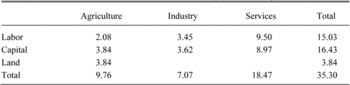
We now describe the construction of the social accounting matrix for the year 1935. Value added by sector, in billions of 1950 Argentine pesos (A$), is from CEPAL. The labor share in each sector is from the 1950 IO matrix. In both cases, the sectors are aggregated into our three sectors of agriculture (including livestock and fisheries), industry (including manufacturing and a very small mining sector), and services (the rest). Sector-specific payments to capital are the residuals in each activity, except in agriculture, where nonlabor income is split half and half between capital and land.
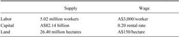
Total supply of labor and land come from CEPAL (1958). The supply of capital is derived by assuming a rental rate of 20 percent. We compute the wage of each factor as the total income of each factor divided by its total supply in the whole economy.
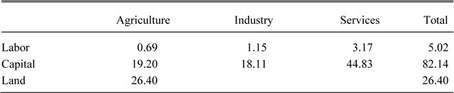
We get factor employment by sector by dividing payment from activity to factor by factor wage, yielding:
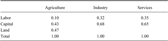
Finally, we get CES share parameters for the production functions from the equation
 \begin{equation}
\delta _{c,f} = \frac{{WfF_{c,f}^{1 + p} }}{{\Sigma f_' \left({Wf_' F_{c,f}^{1 + p} } \right)}}\,{\rm for }c = A,I,S;f = L,K,T
\end{equation}
where variables are defined above with the model. δ c,f is the share parameter of factor f in the CES production function of sector c, Wf is the (economy-wide) wage of factor f, Fc,f is the quantity of factor f used by sector c, and ρc is the exponent parameter in the CES production function of sector c.
We assume a tariff of tm = 23.1 percent following Díaz Alejandro's (Reference Díaz-Alejandro1970, p. 282) estimate for 1935. However, since the relative domestic price of tradables is exogenous and taken from the data in all simulations except for no-ISI, from the point of view of domestic prices we are implicitly assuming the actual changes in trade policy of the period.
VALUE ADDED (A$ BILLIONS) AND LABOR SHARE, 1935

PAYMENTS TO FACTORS BY SECTOR (A$ BILLIONS), 1935

TOTAL FACTOR SUPPLY AND ECONOMY-WIDE PER-UNIT WAGE BY FACTOR, 1935

FACTOR EMPLOYMENT 1935 BY SECTOR

δ c,f FOR SECTORS C AND FACTORS F

The remaining parameters in the model were either determined from the SAM or calibrated, as follows:
-
1. Elasticity of substitution is
$\epsiv = 1 \frac 1 + \rho = 8$
, following Debowicz (Reference Debowicz2010). This implies that ρ = 0.25 in the production functions. -
2. TFP growth in agriculture, industry and services at 0 percent, 1.5 percent, and 1.6 percent respectively.
-
3. Elasticity of land use ε T = 0.1, following Kanyala J. Barr et al. (Reference Barr, Babcock, Carriquiry, Nasser and Harfuch2010).
-
4. Elasticity of labor supply ε L =0.00234, following Roxana Maurizio (2011).
-
5. Armington elasticity is equal to 2 so ρ M = − 5, following Thurlow's (2004) model of South Africa; δM =0.531 is derived from the SAM for 1935.
-
6. Parameters for the LES consumption function are derivedFootnote 20 assuming a Frisch parameter of −2 and elasticities given by GTAP for South AfricaFootnote 21 (0.37 for agropec, 1.06 for industry, and 1.18 for services). We use South Africa because its 2008 GDP is very close to Argentina's 1935–1960 average (using 1990 PPPs from Maddison Reference Maddison2010).
-
7. Average propensity to save μ = 0.257 derived from the input-output matrix for 1950.
-
8. Depreciation δ K = 8 percent (prior of 5 percent).
-
9. Mobility of capital: sensitivity of investment to rental differentials, β K = 12
-
10. Rental rate for the capital stock equal to 20 percent.
-
11. Labor mobility:
-
a. φ = 0.2, i.e. 20 percent of previous period's labor force is mobile;
-
b. sensitivity of mobile labor to wage differentials β L = 5.
-

Appendix 2: Data
To construct sectoral output indices at constant prices, GDP is partitioned into the following three sectors, based on output data from Economic Commission for Latin America (1959) (henceforth ECLA). “Agriculture” includes forestry and livestock farming. “Industry” comprises manufacturing industry and mining. “Services” comprises electricity and other public services, construction, transport, communications, commerce, financial services, ownership of dwellings, general government, and other services. ECLA has data at 1950 prices for 1900–1955. For 1956–1960 we use growth rates implied by output indices at 1960 prices in BCRA (1975, pp. 116–17).
Sectoral output at current prices, which we use along with the constant price data to produce sectoral GDP deflators, is available from 1935. For 1935–1949 we use estimates due to Secretaría de Asuntos Economicos, published in BCRA (1976). For 1950–1960 the source is BCRA (1975). The former data series goes up to 1962 but we use the BCRA series from the earliest point possible because of a reported underestimation in the value of manufacturing by the earlier source (Díaz Alejandro Reference Díaz-Alejandro1970, p. 392). According to the Secretaría, manufacturing comprised between 18 and 22 percent of the value of total GDP over the period 1950–1962, when the two sources overlap, compared with the later BCRA estimate of between 25 and 30 percent.
Wholesale price data are from IEERAL (1986), who use a variety of sources over time. The index starts in 1913 and for 1913–1925 it is based on reported prices in various editions of the Revista de Economia Argentina of the Fundacion Alejandro Bunge. In this period, “non-agriculture” is effectively a subset of manufacturing, comprising a weighted average of the price indices of the following six subsectors: textiles and their derivatives, iron and derivatives, wood and derivatives, non-ferrous metals and derivatives, non-metalic minerals and derivatives, and chemical products (IEERAL 1986, pp. 176–77). For later years, they take the index directly from other historical sources, which we were unable to locate for further details.
Employment data by sector used in Figures 1 and 2 and in the regressions are as follows. For 1900–1947 they are five-year averages from ECLA. From 1948 we use data due to the Consejo Nacional de Desarrollo (CONADE), which are reported in Díaz-Alejandro (Reference Díaz-Alejandro1970). Since there is a jump in levels of between 7 and 12 percent in each of the three sectors where they overlap in 1947–1949, we use the growth rates in the CONADE data applied to the ECLA data. The land variable is defined as total cultivated land, which includes all land used for grains, oilseeds, vegetables, industrial crops, fodder cultivations, and fruits. For 1900–1936 we use Ministerio de Agricultura (1937); for 1937–1962 we use data from the Revista de la Bolsa de Cereales, Numero Estadistico (1963), which are reported in Díaz Alejandro (Reference Díaz-Alejandro1970, p. 442).
Appendix 3: Detailed Simulation Results
SIMULATION RESULTS AS DEVIATIONS FROM BASE SIMULATION (percent)