1. Introduction
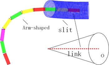
Traditional rigid robots are difficult to perform tasks in narrow spaces. Hyper-redundant robots have great potential for the application in confined space due to their high flexibility and slim body size. Hyper-redundant robots have been widely studied, such as serpentine robot, continuum and soft robot. Inverse kinematics of the hyper-redundant robot is a challenging hot spot in the field. However, high efficient and shape-controllable inverse kinematics of hyper-redundant robots have not yet been solved effectively.
Serpentine robot is snake-like robot composed of multiple small links connected by Hooke’s hinge, such as the segmented linkage robot designed by Tianliang Liu [Reference Liu, Xu, Yang and Li1]. Continuum robots [Reference Yang, Xu, Li and Yu2–Reference Kolachalama and Lakshmanan4] are a jointless robot arm with a biological structure similar to an elephant trunk such as the elephant trunk-like robot developed by Walker [Reference Walker5], the BHA [Reference Rolf and Steil6]. If the material of the continuum robot is soft, it can be classified as an emerging class of bionic soft robots in recent years.
Kinematic modeling: The difficulty lies in the planning problem brought by super-redundant degrees of freedom. For multi-joint continuum robots, which are composed of rigid joints sequentially connected in series, the traditional Denavit-Hartenberg (D-H) [Reference Huang and Jiang7, Reference Yang, Jin, Han, Zhao and Hu8] modeling method can be used for kinematic modeling. Tianliang Liu [Reference Xu, Liu and Li9] conducts kinematic modeling according to the traditional D-H method for a cable-driven continuum robot with multiple rigid links connected by Hooke’s hinge. For jointless continuum robots, the equivalent joint method is often used for kinematics modeling. The equivalent joint method equates the motion of a continuum robot without joints to virtual joints and links, trying to find the kinematics and inverse kinematics using the traditional method. Wang [Reference Wang, Frazelle, Wagner and Walker10] used the virtual joint method to equivalently model a continuum robot with constant curvature and derived its kinematic model using the D-H method. The continuum robot is equated to three rotating and one moving subsets.
Therefore, for continuum and soft robots, scholars have proposed several effective kinematic modeling methods such as the continuous curvature model, the beam model and the Cosserat rod theory. The kinematic modeling of a continuum robot with continuous curvature mainly includes constant curvature methods and non-constant curvature (also known as variable curvature (VC)) methods. Nuelle [Reference Nuelle, Sterneck, Lilge, Xiong, Burgner-Kahrs and Ortmaier11] models the kinematics of a continuum robot using the equivalent arc method based on the assumption of constant curvature. Huang [Reference Huang, Zou and Gu12] simplified the variable curvature forward kinematic model of a continuum robot arm to reduce the computational complexity. Commonly used constant curvature curves include Bessel curves in addition to circular curves. The beam model and the Cosserat rod theory develop a new theory for the characteristics of the continuum robots by equating them to deformed beams or rods to build kinematic models. Dalvand [Reference Dalvand, Nahavandi and Howe13] uses the beam model to model the kinematics of a tendon-driven continuum robot and develops quantitative relationships between the number of tendons, tendon loads, and bending angles. Neumann [Reference Neumann and Burgner-Kahrs14] performs kinematic modeling of a continuum robot using the Cosserat rod model and describes the deformation of the rod using a constant curvature arc and a B spline curve respectively.
Inverse kinematics: A common method for solving the inverse kinematics for redundant robotic arms is the numerical iterative method. In the linkage redundant manipulator designed by Tianliang Liu [Reference Liu, Mu, Xu, Yang, You, Fu and Li15], the kinematics of the manipulator is established using the D-H method. Considering the linkage characteristics of the arm, the Jacobi matrix is simplified and the iterative method is used for inverse kinematics. Mu Zonggao [Reference Mu, Yuan, Xu, Liu and Liang16] proposes a segmented geometry method for the spatial hyper-redundant robot, which geometrically divided the arm into three parts. Then, the kinematics is solved separately according to the segments, thus simplifying the computational process of the inverse kinematics. However, the traditional numerical iterative method based on D-H coordinate system has the outstanding problems of low efficiency and uncontrollable arm shape and is prone to singularity problems, which limit its wide application. The higher the number of joints, the more complex the Jacobi matrix [Reference Kleff and Li17] is and the less efficient the solution is.
In contrast, the geometric method is more efficient and easy to constrain the arm shape, thus widely studied for inverse kinematics of hyper-redundant robots. Chirikjian [Reference Chirikjian18] proposed the concept of backbone curve to describe the configuration of the super-redundant manipulator. The proposed method is computationally less expensive and is suitable for online path planning and real-time control. However, the determination and solution of the backbone function depends on experience and skill. In ref. [Reference Chirikjian and Burdick19], Chirikjian defines the backbone curve as a series of mode functions that can be selected as needed. Once the backbone curve is determined based on the end-effector position, a certain fitting algorithm is used to determine the joint angle. Fahimi [Reference Fahimi, Ashrafiuon and Nataraj20, Reference Fahimi, Ashrafiuon and Nataraj21] used different mode functions to fit the curves, and he applied a recursive fitting algorithm to the gimbal joint to avoid solving a large number of nonlinear equations. Li Sheng [Reference Sheng, Yiqing, Qingwei and Weili22] proposed an alternative geometric approach that allows the solution of a large number of nonlinear equations. Mohamed [Reference Mohamed, Samer Yahya and Yang23] proposed another geometric method that can find a solution from the infinite solution of the super-redundant robotic arm. This method sets the angles of adjacent joints to be equal. It is very effective for simple planar robotic arms with equal link lengths and the singularity problem is avoided. Andreas Aristidou [Reference Aristidou and Lasenby24] introduced the FABRIK geometric iterative method for solving the inverse kinematics. Compared with the traditional method, FABRIK is more the efficient for finding the inverse solution. The traditional FABRIK algorithm cannot solve the inverse kinematics including end roll degrees of freedom. To solve this limitation, Liu Tianliang [Reference Liu, Yang, Xu, Mylonas and Liang25]proposed the double-layer FABRIK algorithm to solve the inverse kinematics of a cable-driven hyper-redundant robot. Joint angle constraints and environmental constraints are considered to constraint the arm shape. Geometric iterative methods are more efficient in solving the inverse kinematics of hyper-redundant robot. However, it still needs further improvement in multiple constraints and efficiency. Recently, artificial neural networks have been used to solve the inverse kinematics problem for robotic arms [Reference Yuqi, Jinjiang, Ranran, Lei and Lei26–Reference Bin, Rong and Jun28]. The size of the training set will vary significantly with the number of degrees of freedom, and the solution is very inefficient on a continuum robotic arm with super-redundant degrees of freedom.
Contributions: In summary, the geometric iterative method has the advantage of high efficiency and is suitable for the inverse kinematics of hyper-redundant robots. However, the traditional geometric iterative method is different to solve the end roll angle inverse kinematics. At present, only ref. [Reference Liu, Yang, Xu, Mylonas and Liang25] uses two-layer nested iterations to solve end roll angle inverse kinematics. However, it results in large arm shape changes and low efficiency. The above-referenced state-of-the-art materials are compared in Table I. Unlike the presented approaches, we provide an efficient and improved FABRIK algorithm to solve full-degree-of-freedom inverse kinematics problems. It mainly has the following contributions.
-
(1) The single-layer improved FABRIK method was developed to solve the position and pointing inverse kinematics considering path, environment and joint angle constraints instead of two-layer method. The efficiency is improved.
-
(2) The virtual arm was established as the constraint space of the real arm based on the geometrical constraints of the environment. By adjusting the parameters of the virtual arm, the planning of the roll angle is achieved. The arm shape can be avoided in large changes.
-
(3) The improved FABRIK method was verified by inverse kinematic planning simulations in narrow space. Results show that the efficiency is greatly improved and the shape of the arm is constrained.
-
(4) The improved FABRIK method was used to realize trajectory tracking and joint angle avoidance limit in narrow space. It has the advantages of simple algorithm and high efficiency.
The rest of this paper is organized as follows. Section 1 presents the preliminary works about kinematics modeling and traditional FABRIK iterative method. In Section 3, we introduce the improved FABRIK method and present the virtual arm to solve planning of roll angle. In Section 4, we introduced trajectory tracking and joint angle avoidance limits in narrow spaces. In Section 5, simulations are carried out to verify the method. Section 6 gives the conclusion.
Comparisons among the state-of-the-art materials.

2. Preliminaries
2.1. Kinematic modeling
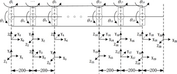
For a multi-joint hyper-redundant robot composed of rigid joints connected sequentially, this paper used a modified D-H coordinate system method to establish a D-H coordinate system with 20 degrees of freedom for 10 modular joints as shown in Fig. 1. The D-H parameters of each joint of the continuum robot arm are obtained according to the rules established in the D-H parameter table, as shown in Table II.
According to the D-H parameter table of the robotic arm system and the rules for the establishment of the D-H coordinate system, the Homogeneous transformation matrix of each joint of the robotic arm
 $^{i-1} T_{i}$
is obtained, and its forward kinematic equations are presented as follows.
 \begin{equation} T_{sn} =^{0} T_{1} ^{1} T_{2} ^{2} T_{3} ^{3} T_{4} \cdots ^{19} T_{20} \end{equation}
where
 $^{i-1} T_{i}$
is the homogeneous transformation matrix between two adjacent coordinate systems of joint segment i.
Multi-joint continuum robot arm D-H parameters.

D-H coordinate system of the continuum robot arm.

2.2. Traditional FABRIK method
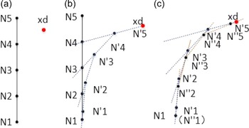
For the inverse kinematic solution problem of multi-joint continuous robot, some scholars have proposed a geometric-based FABRIK method with high efficiency, zero-error solution and no singularity problem. The conventional FABRIK is based on the geometric iterations of forward and backward iterations to quickly find the end position but not the pose, and its algorithm flow chart is shown in Alg. 1. The algorithm process for a four-joint continuum robot is shown in Fig. 2.
Forward arrival iteration: As shown in Fig. 2(a), Ni is the initial joint point, and the end joint point is coincident with the target point N’5 when forward iteration is performed, and N’4 is determined according to the desired end target and the length of the joint segment. The length of N’5 N’4 is equal to N5 N4, and then, the remaining points are determined as shown in Fig. 2(b), such that N’3 is on the line of N’4 N3 and the length of N’4 N’3 is equal to N4 N3, and the remaining points are determined in the same order. Because the forward iteration of the arm joint point N1 is out of the initial point, the backward iteration is needed.
Backward arrival iteration: As shown in Fig. 2(c), similar to the forward iteration, the target point N’5 is taken as the starting point, and N1 is taken as the target point of N’1 in reverse order to find the position of each joint point.
The above process is one FABRIK iteration, and the zero-error solution can be achieved by several iterations.
Traditional FABRIK algorithm

Traditional FABRIK iteration for position. (a) initial position (b) forward iteration (c) backward iteration.

2.3. Two-layer FABRIK method
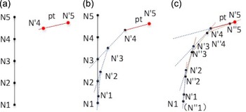
The traditional FABRIK method is difficult to solve the pose tracking, so Tianliang Liu applied two-layer FABRIK method to solve the complete inverse kinematic problem in ref. [Reference Sheng, Yiqing, Qingwei and Weili22]. The inner loop was used to solve the position and pointing, and the outer loop was used to solve the roll angle, and segmented FABRIK method was used to solve the pointing in inner loop. The segmented FABRIK method divided the end joint and the remaining joint into two parts, so end pointing determines the new position of Ni-1 based on the desired position and pointing Pt and then solves the position of other part using the traditional FABRIK method. However, the end link is directly determined along the desired direction, the end joint angle is uncontrollable and the arm shape is not smooth. Moreover, Two-layer iterations have low efficiency. The segmented FABRIK method for position and pointing is shown in Fig. 3
3. Shape-controllable FABRIK method
The traditional method of solving the roll angle cannot control the arm shape, which leads to irregular shape change of the arm and makes it impossible to work properly in extreme environments such as pipelines and other narrow spaces. In this section, we proposed a shape-controllable forward and backward reaching inverse kinematics (SCFABRIK) method to solve the rolling angle, which can control the arm shape within a specific geometric range. The solution efficiency of single-layer iteration is greatly improved compared to traditional double-layer iteration.
3.1. Improved FABRIK method for position and pointing inverse kinematics
The traditional FABRIK method is a geometric iterative method to find the position. In this paper, we proposed an improved FABRIK geometric iterative method that can solve the position and pose simultaneously in a single-layer iteration. Compared with the traditional FABRIK method, we added a pointing rotation iteration after the forward position iteration. Compared with the two-layer iterative algorithm which directly forces the end link to point to the desired direction, the planning joints are smoother. The improved FABRIK method for position and pointing inverse kinematics is shown as Alg. 2.
Improved FARRIK algorithm

Segmented FABRIK method for position and pointing. (a) initial position (b) forward iteration (c) backward iteration.

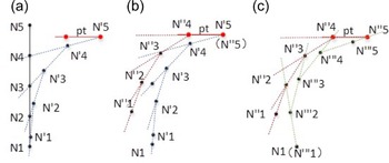
The principle of the algorithm is shown in Fig. 4.
Improved FABRIK geometry iteration method. (a) forward iteration (b) pointing rotation iteration (c) backward iteration.

Unlike the traditional FABRIK forward-backward method, the improved FABRIK method adds a rotation iteration as shown in Fig. 4(b). The 5-degree-of-freedom inverse kinematics solution of the position and pointing can be found by adding this rotation iteration.
3.2. Improved FABRIK method for roll angle inverse kinematics
The design of the super-redundant robot arm is inspired by mollusks such as snakes. Therefore, in solving the inverse solution of the desired roll angle, one can learn from the way a snake wraps around a prism. The end position, pointing and cross-roll angle are constantly changing and conform to certain geometric relationships as the snake wraps around the prism. Moreover, the super-redundant robot can be restricted to the prism.
The positions of virtual and real joint points in the geometry are determined by the following rules.
First, the prism is determined based on the external environment to ensure that the geometry does not come into contact with the external environment.
Then, determine the winding angle
 $\theta$
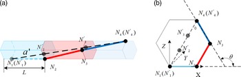
based on the desired roll angle and the current roll angle, and the virtual joint points N’i in each segment of the geometry are selected based on the strait line connecting the base point and end point as shown in Fig. 5.
(a) The position of real joint points and virtual joint points (b) Geometry cross-section.

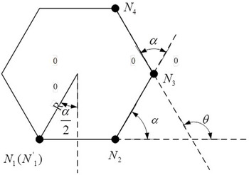
A cross-section of a geometry model.

After, we solve the position and pointing inverse kinematics of the virtual arm.
Finally, the position Ni of real joint points on the geometry can be obtained by wrapping around the prime at the same angle as shown in Fig. 5. The geometric relationship between the real joint points and the geometry is shown in Fig. 6.
The input roll angle is
 $\theta$
 \begin{equation} \theta =\theta _{t} +\Delta \theta \end{equation}
 \begin{equation} \Delta \theta =\theta _{d} -\theta _{t} \end{equation}
The length of the single-segment virtual arm is
 \begin{equation} a{}' =\sqrt{a^{2}-(2R\sin \left(\frac{\alpha }{2} \right)^{2} } \end{equation}
 \begin{equation} \alpha =\theta/(n-1) \end{equation}
where
 $\theta$
is the angle of the entire arm winding prism,
 $\theta _{t}$
is the current roll angle,
 $\alpha$
is the angle of projection of adjacent link on the cross-section of the geometry. roll angle of single joint is
 $\alpha$
,
 $a$
is the length of a single link,
 $a{}'$
is a virtual link length,
 $L$
is the length of the single-segment geometry, and the length of the single-segment virtual arm is a’.
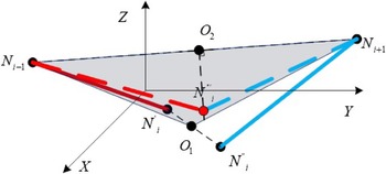
Adjusted joint points, the red solid line and the blue solid line are separated joint segments, the red dashed line and the blue dotted line are the adjusted joint segments.

After obtaining the model of the virtual arm, the improved FABRIK can be used for virtual arm to solve position and pointing. So we can control the motion of the prism by controlling the position and pointing of the virtual arm and then calculate the real joint points based on the position of the real arm on the geometry.
However, the motion of the geometry will lead to the separation of the real joint points. Thus, separated joint points need to be adjusted to the same point and the adjustment method in this paper is shown in Fig. 7.
If
 $ N_{i}$
is separated into two points
 $N{}' _{i} N{}'{}' _{i}$
among the three joint points of
 $N_{i-1} N_{i} N_{i+1}$
, take the midpoint of
 $N{}' _{i} N{}'{}' _{i}O_{1}$
to form the plane
 $ N_{i-1} O_{1} N_{i+1}$
and make a line perpendicular to
 $N_{i-1} N_{i+1}$
on the plane
 $N_{i-1} O_{1} N_{i+1}N{}'{}'{}' _{i}$
, where the length of
 $O_{2} N{}'{}'{}' _{i}$
is equal to real arm length. This method can effectively adjust the separated joint points, and the adjusted points will be as close to the range of the geometry as possible.
The length of the virtual robotic arm proposed in this method will change with the data of the geometry. So the arm length needs to be updated in iterations. The algorithm is shown as Alg. 3.
4. Joint limit avoidance and trajectory planning
4.1. Joint limit avoidance
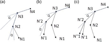
We improved a geometric method for limit avoidance of joint angles based on improved FABRIK as Fig. 8.
Traditional geometric limit avoidance methods only adjust joint points where the joint angle exceeds the limit angle. In some cases, this reduces the continuity of the entire arm, resulting in non-convergence in the process of avoiding the limit, and thus no solution.
The method we proposed is to start at the joint point that exceeds the limit angle of the joint and rotate the remaining arm as the joint point rotates, as shown in Fig. 8. This guarantees continuity throughout the arm and does not diverge over the course of iteration in some cases.
Virtual arm method to find the pose

Joint angle avoidance limit. (a) Initial arm angle. (b) First step iteration of joint avoidance limit. (c) Joint Avoidance Limit Step 2 Iteration.

Trajectory tracking in confined spaces and the cone is the range of end joint deflection angles.

4.2. Trajectory planning
The robotic arm works in a narrow space and it is necessary to realize that the arm tracks the trajectory. During this process, the arm must not touch the obstacle. Figure 9 shows the trajectory tracking process in confined spaces. We proposed a geometric method based on improved FABRIK that can achieve the goal well.
Taking advantage of the continuity of the improved FABRIB method, the arm shape is automatically adjusted according to the change of the path trajectory during the tracking trajectory, and when the arm touches an obstacle, the influence of the end pose on the arm shape is used to adjust the arm shape. When the end pose is determined or cannot meet the obstacle avoidance, the pose of the previous link is adjusted, so as to achieve the goal of fast obstacle avoidance in trajectory tracking. The algorithm flow is shown in Alg. 4 where
 $ d_{i}$
is the distance from each joint point to the path trajectory,
 $d{}'$
is the maximum distance from a joint point to a path trajectory.
Trajectory tracking

5. Results
5.1. Simulations of improved FARRIK method
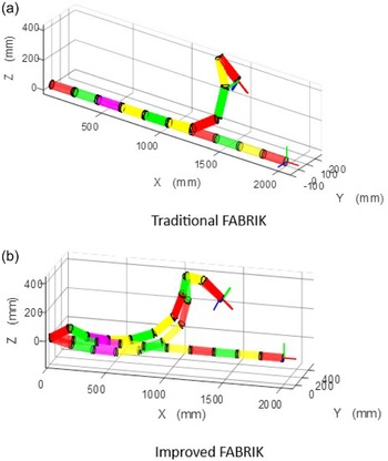
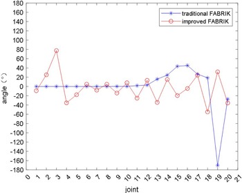
We carried out inverse kinematic simulations based on the traditional method and the proposed method in this paper respectively and compared the maximum joint angle changes. The proposed method has better continuity and less variation, as shown in Fig. 10.
From Fig. 11, it is easy to find that the traditional method does not take into account the pointing iteration, but directly aligns the end link to the end desired direction. Therefore, the traditional method leads to a large variation of the joint angle, which is close to 180
 $^{\circ }$
. In contrast, the joint angle of the method in this paper does not exceed 80
 $^{\circ }$
.
We made a table to compare the advantages of the method in this article as shown in Table III, where N is the number of iterations and the time only counts the iteration time.
In summary, the improved FABRIK geometric iterative method inherits and retains the advantages of the FABRIK geometric method in terms of high efficiency, zero-error solution and no singularity problem; it also solves the problem that the FABRIK method cannot find the pose and the end joint angle of the improved FABRIK method is too large.
5.2. Simulations of joint angle avoidance limit
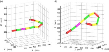
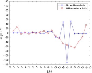
Select random desired target points and use the improved FABRIK algorithm to solve the desired joint position. The simulation is shown in Fig. 12(a). The simulation after adding joint limit avoidance is shown in Fig. 12(b). The joint angles are shown in Fig. 13.
From Fig. 13, it is easy to find that the joint angle obtained by the limit avoidance method in this paper does not exceed 65
 $^{\circ }$
instead of the original close to 140
 $^{\circ }$
.
The results of a comparison of the two methods.

Inverse kinematics simulations of traditional FABRIK and improved FARRIK method.

Comparison of joint angle. The blue curve shows the joint angles using the tradition FRBRIK. The red curve shows the joint angles using the improved FRBRIK proposed in this paper.

5.3. Simulations of arm shape planning
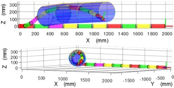
We used pipes to simulate obstacles to observe the arm shape. As shown in Fig. 14, the robotic arm can complete the inverse solution under the condition of obstacle constraints. The table to compare the advantages of the method in this article is shown in Table IV.
Comparative simulations of joint angle avoidance. (a) Joint position without limit avoidance. (b) Joint position with limit avoidance.

Comparison of joint avoidance limit. The blue curve shows the joint angles without joint angle avoidance. The red curve shows the joint angles with joint angle avoidance.

The results of a comparison of the two methods.

Different perspectives of simulation of geometric constraints for inverse solution.

The sample variance is calculated as Eq. (6).
 \begin{equation} S^{2} =\sum _{i=1}^{n} (\theta _{i} -\bar{\theta } )^{2}/n \end{equation}
From the above simulation, it is easy to see that in the process of solving the inverse kinematics of the manipulator, the arm shape can be well constrained within a certain range.
5.4. Simulations of trajectory tracking
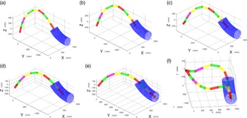
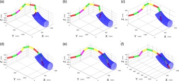
We implement trajectory tracking based on the improved FABRIK method. Only the solution for the end 5 degrees of freedom can be achieved as shown in Fig. 15(a)–(e). However, traditional methods fail to solve the roll angle problem as shown in Fig. 15(f). The arm hits the pipe.
Trajectory tracking based on the improved FABRIK.

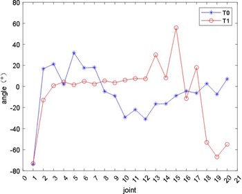
Figure 16 shows the change of joint angle based on traditional methods. From Fig. 17, we can find the end three angles of the red curve are big which causes the collision with the pipe.
The change of joint angle during roll angle solution based on traditional methods. The blue curve is the joint angles in the simulation of 5-degree-of-freedom inverse kinematics at T0. The red curve is the joint angles in the simulation of 6-degree-of-freedom inverse kinematics at T1.

Trajectory tracking based on the SCFABRIK.

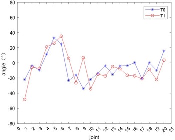
The change of joint angle during roll angle solution based on SCFABRIK methods. The blue curve is the joint angles in the simulation of 5-degree-of-freedom inverse kinematics at T0. The red curve is the joint angles in the simulation of 6-degree-of-freedom inverse kinematics at T1.

We implemented trajectory tracking for the terminal 6-degree-of-freedom solution based on the SCFABRIK, and in the process of solving the roll angle, the arm shape is well controlled in a narrow space. The trajectory tracing based on the SCFABRIK method is shown in Fig. 17.
Figure 18 shows the change of joint angle based on SCFABRIK methods and we can find the angles of the red curve are close to the blue curve which provides good continuity in the shape of the arm.
From the above simulation results, it can be seen that the proposed method can effectively and quickly realize the end 6-degree-of-freedom inverse solution in narrow space and the arm shape is controlled, achieving a good continuity effect.
6. Conclusion
In this paper, we improved the FABRIK method, proposed a SCFABRIK inverse kinematics solution method based on geometric constraints and analyzed kinematics modeling, geometric model and virtual manipulator; then, trajectory tracking in narrow space and joint avoidance limit were introduced; finally, we carried out MATLAB simulation and shared the code to the readers for ease of use [Reference Niu29]. The main research results achieved are as follows:
-
(1) We analyzed the limitation of FABRIK that only solves position and improved the method and proposed improved FABRIK so that it can solve the position and pointing; it also solves the problem of end joint angle being too big caused by the traditional method in the process of re-finding the pointing.
-
(2) In view of the working requirements of ultra-redundant robotic arms in narrow environments and requiring rolling angles, we established a geometric model to constrain the arm shape of the robotic arm within a controllable range, realizing the need to work in a narrow space.
-
(3) Based on the improved method, we did trajectory tracking and joint angle limit avoidance to realize the work of the robotic arm in a narrow space.
The limitation of the proposed method is complex. The proposed method needs to build virtual arm, derive the relationship between the virtual arm and the real arm, and solve the joint position of the actual joint point on the virtual arm.
As a special robot, the ultra-redundant robotic arm involves knowledge in many disciplines and fields knowledge, and its research has certain prospect significance. In the future, further research should include:
-
(1) The research on the effective obstacle avoidance planning algorithm of the robotic arm in three-dimensional space is helpful to carry out efficient planning and control of different tasks and improve its environmental adaptability in different environments.
-
(2) Research on the autonomy and intelligence of robotic arm system. In-depth study of multi-sensor fusion technology of robotic arm system to realize its autonomous intelligent control in unknown and complex environment to ensure the completion of tasks in small unknown environment.
Author contributions
Pingan Niu and Liang Han designed the study. Pingan Niu carried out the experiments. Liang Han and Yunzhi Huang calibrated English expression. Pingan Niu wrote the article. Liang Han and Lei Yan did the review and guidance.
Financial support
This work was supported by National Natural Science Foundation of China (Grant No. 62273129, Grant No. 62203147), Anhui Provincial Key Research and Development Project (Grant No. 2022a05020025), the Fundamental Research Funds for the Central Universities of China (Grant No. JZ2022HGTA0339).
Competing interests
There are no competing interests.