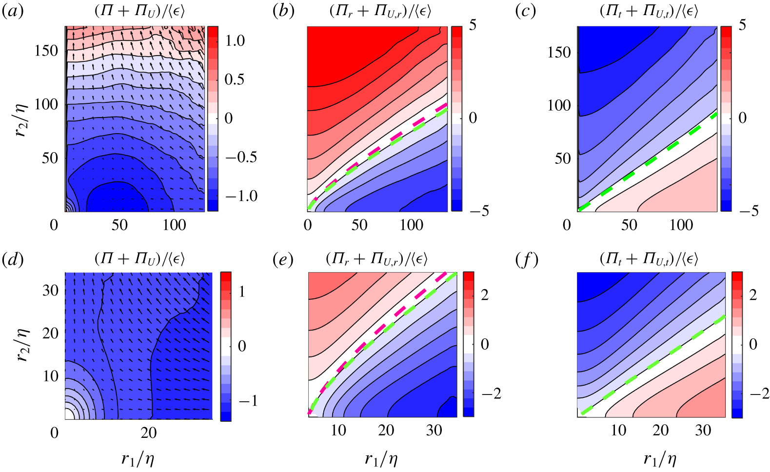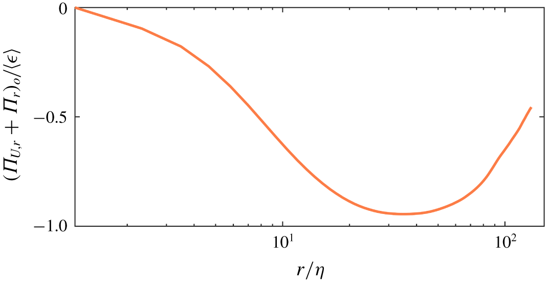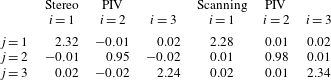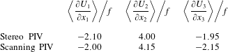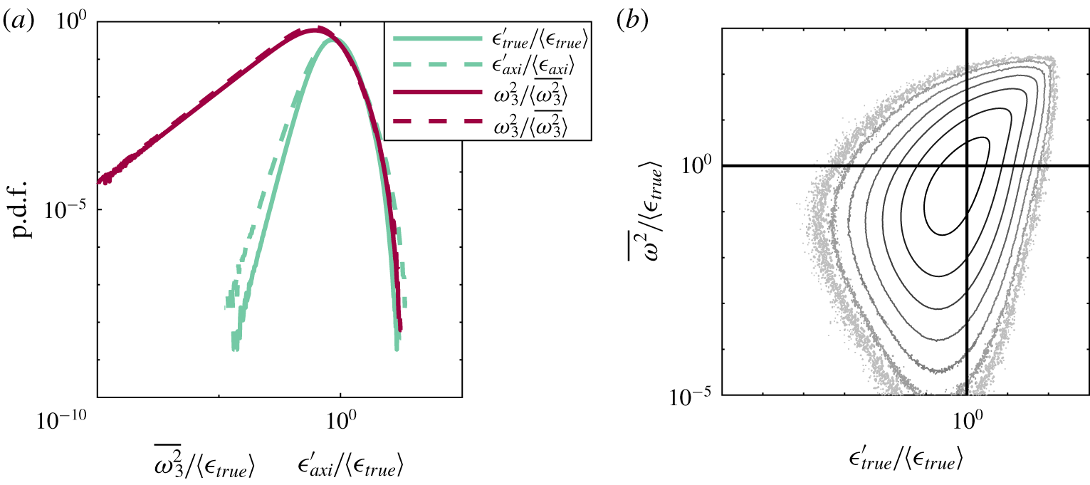

1 Introduction
Turbulent flows are characterised by their unsteady, three-dimensional motion across a wide range of length and time scales. The observation of small-scale motion in flows containing energy injection at only the large scale prompted the classical concept of an energy cascade (Richardson Reference Richardson1926), where energy is transferred to increasingly fine-scale motion, until viscosity finally limits the process through dissipation, turning the kinetic energy into heat. Since the energy cascade was introduced, energy transfer in turbulent flows has remained an ongoing subject of investigation for decades (Kolmogorov Reference Kolmogorov1941; Batchelor Reference Batchelor1969; Godeferd & Cambon Reference Godeferd and Cambon1994; Smith & Waleffe Reference Smith and Waleffe1999; Cimarelli et al. Reference Cimarelli, De Angelis, Jiménez and Casciola2016). Energy transfer equations were originally derived using assumptions of homogeneity and isotropy for mathematical convenience, but despite numerous attempts to recreate such properties in the laboratory (Monin & Yaglom Reference Monin and Yaglom1975), such properties are rarely found in real flows. Therefore, a number of studies have focused on understanding the effects of anisotropy, scale dependence and inhomogeneity on energy transfer. The effect of mean flow gradients was considered by Deissler (Reference Deissler1961, Reference Deissler1981), who through spectral analysis of general inhomogeneous turbulence concluded that not only turbulent self-interactions, but also interactions between turbulent fluctuations and the mean flow are sources of inter-scale energy transfer, thus transferring energy from larger to smaller scales, or in the opposite direction. Further to this, Danaila et al. (Reference Danaila, Anselmet, Zhou and Antonia1999) suggested a modified version of Kolmogorov’s  $-4/5\text{th}$ law, which is derived for homogeneous, isotropic turbulence, by arguing that in many real and laboratory flows, the Reynolds number is not large enough to fully separate the small scales from the large scales, and that large-scale and inhomogeneity effects would therefore affect the energy transfer. In this study, an inhomogeneity term was added to the equation to make up for non-stationary moments of the velocity increments. Later studies by this group also considered a mean flow consisting of predominantly one component, which is varying only in one direction (Danaila et al. Reference Danaila, Anselmet, Zhou and Antonia2001; Danaila, Anselmet & Antonia Reference Danaila, Anselmet and Antonia2002), which would be the case in, for example, a channel flow. This allowed the effect of mean shear on the scale-by-scale energy budget to also be included, resulting in a production term in the inter-scale energy equation. Hill (Reference Hill2002) derived from the incompressible Navier–Stokes equation, a formulation that can systematically assess all such contributions to the overall deviation from Kolmogorov’s
 $-4/5\text{th}$ law, including inhomogeneity, anisotropy, unsteadiness and large-scale effects. This evolution equation of the second-order structure function is a fully generalised version of the Kármán Howarth equation (von Karman & Howarth Reference von Karman and Howarth1938) which was originally derived for homogeneous, isotropic flows. The equation is sometimes referred to as the Kármán–Howarth–Monin–Hill (KHMH) equation, and through its application, it is possible to describe the total flow of energy both in physical space and across spatial scales for any flow.
Recent studies have used this equation as a framework to investigate the transfer of energy in a range of different turbulent flows. Casciola et al. (Reference Casciola, Gualtieri, Benzi and Piva2003) used a variant of the Kármán Howarth equation for homogeneous, anisotropic turbulence to study a homogeneous shear flow using direct numerical simulations (DNS). Similarly, a weak formulation of the Kármán Howarth Monin equation was used by Debue et al. (Reference Debue, Shukla, Kuzzay, Faranda, Saw, Daviaud and Dubrulle2018b) for investigating the effects of quasi-singularities or singularities in a von Kármán flow, and found that the extreme events of the instantaneous inter-scale energy transfer govern the intermittency corrections given in the refined similarity hypothesis (Kolmogorov Reference Kolmogorov1962; Oboukhov Reference Oboukhov1962). Fully generalised versions of the Kármán Howarth equation have also been used in studies of anisotropic and inhomogeneous turbulence to study cascade behaviour in a rotating flow (Campagne et al. Reference Campagne, Gallet, Moisy and Cortet2014), the relations between global and local energy transfers in a von Kármán flow (Kuzzay, Faranda & Dubrulle Reference Kuzzay, Faranda and Dubrulle2015), in the near field region behind a grid (Gomes-Fernandes, Ganapathisubramani & Vassilicos Reference Gomes-Fernandes, Ganapathisubramani and Vassilicos2015; Valente & Vassilicos Reference Valente and Vassilicos2015) and the planar wake generated by a square prism (Portela, Papadakis & Vassilicos Reference Portela, Papadakis and Vassilicos2017). A common feature in the majority of these previous studies is that mean flow contributions to the inter-scale energy budget are negligible, with the exception of the study by Portela et al. (Reference Portela, Papadakis and Vassilicos2017), where gradients in the mean flow are present. In the absence of mean flow, contributions to the scale-to-scale transport often focus on the nonlinear contribution, with all studies demonstrating some degree of inter-scale anisotropy. Furthermore, although the globally spherically averaged transfer of energy is in the forward cascade direction, defined such that energy is transported from larger to smaller scales, with the exception of Valente & Vassilicos (Reference Valente and Vassilicos2015) these studies also all contain regions in scale space of locally inverse cascade behaviour, where energy is transferred from smaller to larger scales. Similarly Carter & Coletti (Reference Carter and Coletti2018) investigated energy transfer in a jet-stirred turbulent flow, and observed anisotropy in the rate of energy transfer, despite well controlled flow homogeneity. Based on these recent studies, it appears that the nonlinear inter-scale energy transfer in different flows varies significantly, and at present it is still uncertain how flow homogeneity and anisotropy in different flows relates to the scale-space orientation of the energy transfer, and if inverse cascade behaviour is omnipresent, or if the examples above represent exceptional cases.
In this work, we have performed a detailed study of the energy transfer of the flow between two counter-rotating disks or impellers, often referred to as a von Kármán flow. The flow has been studied in a large number of analytical (Batchelor Reference Batchelor1951; Stewartson Reference Stewartson1953; Zandbergen & Dijkstra Reference Zandbergen and Dijkstra1987), numerical (Mordant, Lévêque & Pinton Reference Mordant, Lévêque and Pinton2004; Kreuzahler et al. Reference Kreuzahler, Schulz, Homann, Ponty and Grauer2014; Nore et al. Reference Nore, Castanon, Cappanera and Guermond2018) and experimental studies (Bonn et al. Reference Bonn, Couder, van Dam and Douady1993; Cadot, Douady & Couder Reference Cadot, Douady and Couder1995; Voth, Satyanarayan & Bodenschatz Reference Voth, Satyanarayan and Bodenschatz1998; Bourgoin et al. Reference Bourgoin, Volk, Plihon, Augier, Odier and Pinton2006; Ouellette et al. Reference Ouellette, Xu, Bourgoin and Bodenschatz2006; López-Caballero & Burguete Reference López-Caballero and Burguete2013; Lawson & Dawson Reference Lawson and Dawson2015; Debue et al. Reference Debue, Shukla, Kuzzay, Faranda, Saw, Daviaud and Dubrulle2018b; Podvin & Dubrulle Reference Podvin and Dubrulle2018; Lawson et al. Reference Lawson, Bodenschatz, Knutsen, Dawson and Worth2019), and the set-up is ideal for laboratory experiments as high Reynolds numbers can be achieved in relatively small laboratory spaces. The mean flow of the tank has been reported to be anisotropic and inhomogeneous (Porta et al. Reference Porta, Voth, Moisy and Bodenschatz2000) but the turbulent fluctuations at the very centre of the tank can be considered to be locally homogeneous based on second-order metrics (Jucha Reference Jucha2014; Lawson & Dawson Reference Lawson and Dawson2014). Given the widespread use of this configuration in understanding the small-scale structure of turbulent flows, it is of significant interest to study the transfer of energy in this apparatus.
The aim of this study is to use the full KHMH equation to investigate the inter-scale energy budget and cascade behaviour in the well known axisymmetric homogeneous flow generated by a von Kármán mixing tank. In particular we are interested in understanding: Does the energy transfer in this flow share the same directional dependency or anisotropy as other flows, and will this nominally statistically homogeneous axisymmetric flow also exhibit regions of inverse cascade behaviour such as observed by Qu, Bos & Naso (Reference Qu, Bos and Naso2017) in direct numerical simulations of purely axisymmetric turbulence? Which processes are significant to balance the energy budget at the various scales captured by the experiments? Given the flow at the centre of von Kármán tanks have a very small mean component relative to turbulent fluctuations, but with strong stationary gradients in all flow directions, how significant is the linear inter-scale energy transfer?
A secondary objective of the current work is to leverage the recent development of highly accurate and fully volumetric experimental methods (Lawson & Dawson Reference Lawson and Dawson2015). For many decades researchers had to rely on measurements made at a single point in the flow, and often only consider a single component of velocity (Pao Reference Pao1965; Shen & Warhaft Reference Shen and Warhaft2002). More recently multi-component planar measurements have become widely available (Campagne et al. Reference Campagne, Gallet, Moisy and Cortet2014; Debue et al. Reference Debue, Shukla, Kuzzay, Faranda, Saw, Daviaud and Dubrulle2018b). However, all such studies require the use of symmetry assumptions (Gomes-Fernandes et al. Reference Gomes-Fernandes, Ganapathisubramani and Vassilicos2015) to complete their description of inherently three-dimensional quantities such as the dissipation rate; a process which can be misleading (Thoroddsen Reference Thoroddsen1995). In the present work we use fully volumetric measurements, which allows us for the first time to experimentally investigate energy transfer using the KHMH equations without the use of assumptions or surrogates on which planar or point-wise measurements must rely (Thiesset et al. Reference Thiesset, Danaila, Antonia and Zhou2011; Gomes-Fernandes et al. Reference Gomes-Fernandes, Ganapathisubramani and Vassilicos2015; Kuzzay et al. Reference Kuzzay, Faranda and Dubrulle2015; Carter & Coletti Reference Carter and Coletti2018). The current investigation therefore employs both planar stereoscopic and full volumetric particle image velocimetry (PIV), and the use of very large experimental data sets (200 000 and 40 000 samples from scanning and stereo PIV respectively) in order to converge the higher-order statistics.
Following an introduction of the notation and coordinate systems used in the paper given in § 2.1, a detailed description of the experimental methodology is presented in § 2.2, a brief flow characterisation is outlined in § 2.3 and details of the method used for calculating the inter-scale energy budget are described in § 2.4. Following this, the distribution and transfer of energy is assessed in detail in § 3. Here, we begin by assessing the energy distribution and flux of energy in §§ 3.1 and 3.2. The contribution of the nonlinear transfer term to the energy budget is discussed in § 3.3.1, before including the impact of the linear transfer term in § 3.3.2. In § 3.3.3 we focus on the way in which the energy budget is balanced, and take a closer look at local homogeneity in § 3.4, before some conclusions are drawn.
2 Methodology
Data for this study were obtained using both volumetric scanning PIV and planar stereo PIV. Here, the notation, the experimental facility and methods are presented in addition to details on the vector field processing, a brief flow characterisation and an introduction to the inter-scale energy budget.
2.1 Notation and coordinate system
This section aims to provide an overview of the notation in this work. In the present work the instantaneous velocity field  $\boldsymbol{{\mathcal{U}}}(\boldsymbol{x},t)$ is Reynolds decomposed into the time averaged,
 $\boldsymbol{U}(\boldsymbol{x})$, and fluctuating components,
 $\boldsymbol{u}(\boldsymbol{x},t)$. Similarly, the instantaneous pressure field
 $\mathscr{P}(\boldsymbol{x},t)$ is decomposed into a fluctuating,
 $p(\boldsymbol{x},t)$, and a mean part,
 $P(\boldsymbol{x})$. We shall primarily be concerned with various averages of two-point measurements. The two points are denoted
 $\boldsymbol{x}^{+}$ and
 $\boldsymbol{x}^{-}$. We use superscripts + and - to denote quantities evaluated at
 $\boldsymbol{x}^{+}$ and
 $\boldsymbol{x}^{-}$. The points are centred at position at
 $\boldsymbol{x}=(\boldsymbol{x}^{+}+\boldsymbol{x}^{-})/2$ and are separated by a distance
 $r=|\boldsymbol{r}|$, where
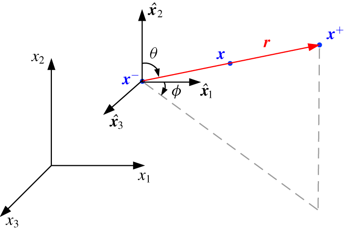
 $\boldsymbol{r}=\boldsymbol{x}^{+}-\boldsymbol{x}^{-}$. This configuration is illustrated in figure 1. Cartesian coordinates are indexed
 $(1,2,3)$, and are associated with unit vectors
 $\hat{\boldsymbol{x}}_{1},\hat{\boldsymbol{x}}_{2},\hat{\boldsymbol{x}}_{3}$, marked in figure 2. Later, it shall be convenient to express separations
 $\boldsymbol{r}$ in terms of polar coordinates
 $(r,\unicode[STIX]{x1D703},\unicode[STIX]{x1D719})$, where the polar direction is aligned with
 $\hat{\boldsymbol{x}}_{2}$ and the azimuth is measured from
 $\hat{\boldsymbol{x}}_{1}$ as shown in figure 1. Similarly these are associated with unit vectors
 $\hat{\boldsymbol{r}}$,
 $\hat{\unicode[STIX]{x1D73D}}$ and
 $\hat{\unicode[STIX]{x1D753}}$ and vector components are indicated with subscripts
 $r,\unicode[STIX]{x1D703},\unicode[STIX]{x1D719}$.
Schematic of the relative configuration of the considered points, vectors and coordinate systems.

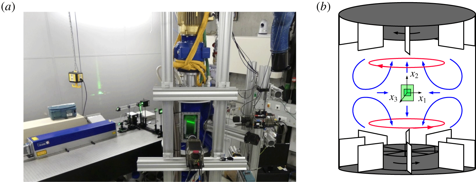
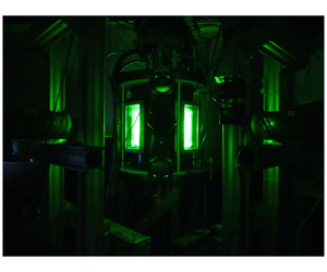
(a) Experimental set-up with laser, optical configuration, flow facility and cameras. (b) Schematic of flow facility, with decomposition of the mean flow between the two counter-rotating impellers: shear layer (——, red) and recirculation due to Ekman pumping (——, blue). The two measurement volumes are marked in green, and the coordinate system  $(x_{1},x_{2},x_{3})$ is given.

We are interested in quantities, e.g. velocity increments  $\unicode[STIX]{x1D6FF}\boldsymbol{u}(\boldsymbol{x},\boldsymbol{r},t)=\boldsymbol{u}(\boldsymbol{x}^{+},t)-\boldsymbol{u}(\boldsymbol{x}^{-},t)$, which are a function of both position
 $\boldsymbol{x}$ in physical space and separation
 $\boldsymbol{r}$ in scale space. Whenever a reference is made to the behaviour of a given quantity in the physical space, the
 $\boldsymbol{x}$ dependence is meant, while the behaviour in scale space should be understood in terms of
 $\boldsymbol{r}$ dependence. The derivatives
 $\unicode[STIX]{x2202}/\unicode[STIX]{x2202}r_{i}$ and
 $\unicode[STIX]{x2202}/\unicode[STIX]{x2202}x_{i}$ are related by
 $$\begin{eqnarray}\left.\begin{array}{@{}c@{}}\displaystyle \frac{\unicode[STIX]{x2202}}{\unicode[STIX]{x2202}x_{i}^{+}}=\frac{\unicode[STIX]{x2202}}{\unicode[STIX]{x2202}r_{i}}+\frac{1}{2}\frac{\unicode[STIX]{x2202}}{\unicode[STIX]{x2202}x_{i}},\quad \frac{\unicode[STIX]{x2202}}{\unicode[STIX]{x2202}x_{i}^{-}}=-\frac{\unicode[STIX]{x2202}}{\unicode[STIX]{x2202}r_{i}}+\frac{1}{2}\frac{\unicode[STIX]{x2202}}{\unicode[STIX]{x2202}x_{i}},\\ \displaystyle \frac{\unicode[STIX]{x2202}}{\unicode[STIX]{x2202}x_{i}}=\frac{\unicode[STIX]{x2202}}{\unicode[STIX]{x2202}x_{i}^{+}}+\frac{\unicode[STIX]{x2202}}{\unicode[STIX]{x2202}x_{i}^{-}},\quad \frac{\unicode[STIX]{x2202}}{\unicode[STIX]{x2202}r_{i}}=\frac{1}{2}\left(\frac{\unicode[STIX]{x2202}}{\unicode[STIX]{x2202}x_{i}^{+}}-\frac{\unicode[STIX]{x2202}}{\unicode[STIX]{x2202}x_{i}^{-}}\right),\end{array}\right\}\end{eqnarray}$$
where summation over repeated indices is implied. Note that all figures in the next section which show the distribution of terms in scale space are also provided in log-axis in the supplementary material, available at https://doi.org/10.1017/jfm.2020.277, together with the data required to reproduce these figures.
Three types of averaging operator are used: the time average, the spatial average and the spherical average. We denote the time average of a signal  $g(\boldsymbol{x},\boldsymbol{r},t)$ as
 $\overline{g}$ and define
 $$\begin{eqnarray}\overline{g}(\boldsymbol{x},\boldsymbol{r},T)=\frac{1}{T}\int _{0}^{T}g(\boldsymbol{x},\boldsymbol{r},t)\,\text{d}t.\end{eqnarray}$$
This is experimentally approximated by an average over  $N_{s}$ samples. Since the number of samples is large and acquired continuously over several days, we shall subsequently drop the explicit dependence upon
 $T$ in our notation. Spatial averages are denoted with angled brackets
 $\langle g\rangle$ and defined
 $$\begin{eqnarray}\langle g\rangle ({\mathcal{A}},\boldsymbol{r},t)=\frac{1}{|{\mathcal{A}}|}\int _{{\mathcal{A}}}g(\boldsymbol{x},\boldsymbol{r},t)\,\text{d}\boldsymbol{x},\end{eqnarray}$$
where  ${\mathcal{A}}$ is the domain over which we measure
 $g$, in this case a region of approximately homogeneous turbulence near the geometric centre of the mixing tank. Additionally,
 $\unicode[STIX]{x2202}{\mathcal{A}}$ is the boundary of
 ${\mathcal{A}}$. Since this region is fixed for the purposes of our experiment, we shall subsequently drop the dependence upon
 ${\mathcal{A}}$ from our notation. Finally, a spherical average is denoted by
 $\langle g\rangle _{\circ }(\boldsymbol{x},r,t)$ and is defined
 $$\begin{eqnarray}\langle g\rangle _{\circ }(\boldsymbol{x},r,t)=\frac{1}{4\unicode[STIX]{x03C0}r^{2}}\iint _{|\boldsymbol{r}|=r}f(\boldsymbol{x},\boldsymbol{r},t)\,\text{d}S_{\boldsymbol{r}}\end{eqnarray}$$
and can be interpreted as the average of  $g$ over the surface of a sphere
 $|\boldsymbol{r}|=r$. The spherical average operation requires three-dimensional data, and for the scanning PIV data, the spherical average of the various terms are calculated directly. For the stereo PIV data, only data in a plane are available, and thus statistical axisymmetry is invoked to estimate spherical averages.
2.2 Experimental set-up
The full experimental set-up used in this study consists of a von Kármán mixing tank, a laser with an optical set-up to guide the laser beam and a pair of high speed cameras. Figure 2(a) shows an overview image of the set-up used for the scanning PIV experiment. The set-up is the same as described by Lawson et al. (Reference Lawson, Bodenschatz, Knutsen, Dawson and Worth2019), but is presented here in more detail.
The mixing tank, illustrated in figure 2(b), consists of a stainless steel cylinder with a height of 58 cm and diameter of 48 cm, with two counter-rotating impellers of diameter 25 cm, located in the top and bottom of the tank. The impellers have 8 baffled vanes of height 5 cm to increase the production of turbulence. The rotational speed of the impellers is maintained at 0.2 Hz, which results in constant energy injection at the largest flow scale. The cylinder is closed by two cooling plates which maintain a fixed water temperature of  $21.2\,^{\circ }\text{C}$, resulting in a kinematic viscosity
 $\unicode[STIX]{x1D708}=0.975~\text{mm}^{2}~\text{s}^{-1}$. Between the impellers and the cylindrical wall, eight static baffle plates are placed to suppress the large-scale rotational motion that would otherwise occur, and to further increase the production of turbulence. The measurement volumes from the stereo and scanning PIV experiments are marked schematically in green in figure 2(b), where the small square illustrates the volumetric measurements. The measurements are made at the geometric centre of the tank, where the mean flow velocity vanishes. The origin of the coordinates system
 $(x_{1},x_{2},x_{2})$ is also located in the geometric centre of the tank, while the axial direction coincides with
 $\hat{\boldsymbol{x}}_{2}$.
The laser beam passes through an optical set-up consisting of two guiding mirrors, a (dynAXIS XS, Scanlab GmbH) galvanometer, followed by sheet forming optics, before passing through the measurement volume. A beam dump minimises back scattered light into the tank. For the stereo PIV, the galvanometer was exchanged with a regular guiding mirror. For both experiments the laser light was used to illuminate the flow through light scattered from  $6~\unicode[STIX]{x03BC}\text{m}$ diameter polymethyl methacrylate (PMMA) microspheres with specific gravity 1.22, which act as passive flow tracers (Stokes number of
 $St=6\times 10^{-5}$).
Two Phantom v640, 4 megapixel cameras were used for both the stereo and scanning PIV experiments. The full image of  $2560\times 1600$ pixels was used for the stereo PIV measurements, while a smaller section of the camera sensor of
 $512\times 512$ pixels was used in the scanning PIV experiments due to limitations in the data uploading time.
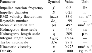
Flow parameters and calculated length and time scales, where RMS is the root-mean-square value.

With the exception of the optics, the set-up for the two experiments were identical. An overview of the experimental parameters is given in table 1. The Taylor microscale is estimated using the following relation, which is derived for isotropic flows:
 $$\begin{eqnarray}\unicode[STIX]{x1D706}^{2}=\frac{15\unicode[STIX]{x1D708}\langle u_{rms}\rangle ^{2}}{\langle \unicode[STIX]{x1D716}\rangle },\end{eqnarray}$$
where  $\langle u_{rms}\rangle$ is the spatial average of the RMS fluctuating velocity
 $u_{rms}(\boldsymbol{x})=\sqrt{\frac{1}{3}\overline{u_{i}(\boldsymbol{x},t)u_{i}(\boldsymbol{x},t)}}$, and
 $\unicode[STIX]{x1D716}(\boldsymbol{x})=\unicode[STIX]{x1D708}\overline{((\unicode[STIX]{x2202}u_{i}(\boldsymbol{x},t))/\unicode[STIX]{x2202}x_{j})((\unicode[STIX]{x2202}u_{i}(\boldsymbol{x},t))/\unicode[STIX]{x2202}x_{j})}$ represents dissipation of kinetic energy of turbulence. It is important to note that
 $\unicode[STIX]{x1D716}$, as defined here, is the so-called pseudo-dissipation. This is in opposition to the true dissipation,
 $\unicode[STIX]{x1D716}_{true}=2\unicode[STIX]{x1D708}\overline{\unicode[STIX]{x1D634}_{ij}\unicode[STIX]{x1D634}_{ij}}$, where
 $\unicode[STIX]{x1D634}_{ij}=\frac{1}{2}((\unicode[STIX]{x2202}u_{i}/\unicode[STIX]{x2202}x_{j})+(\unicode[STIX]{x2202}u_{j}/\unicode[STIX]{x2202}x_{i}))$. The difference between the two is usually small, and thus often neglected for the sake of the equations simplicity (Pope Reference Pope2005). In the present work we are consequently using
 $\unicode[STIX]{x1D716}$, and refer to it as dissipation (except for appendix B, where
 $\unicode[STIX]{x1D716}_{true}$ is utilised). The longitudinal integral length scale,
 $L_{LL}$, is estimated using (2.6) applying the procedure described in Jong et al. (Reference Jong, Cao, Woodward, Salazar, Collins and Meng2009) (the spatial averaging is applied because the involved statistics are homogeneous to a large extent, as has been confirmed in auxiliary checks):
 $$\begin{eqnarray}L_{LL}=\int _{0}^{\infty }\left\langle \frac{R_{LL}(\boldsymbol{x},r)}{R_{LL}(\boldsymbol{x},0)}\right\rangle \text{d}r\approx \int _{0}^{r_{max}}\left\langle \frac{R_{LL}(\boldsymbol{x},r)}{R_{LL}(\boldsymbol{x},0)}\right\rangle \text{d}r+\frac{A}{B}\text{e}^{-Br_{max}},\end{eqnarray}$$
where  $R_{LL}(\boldsymbol{x},r)$ is the longitudinal autocorrelation function
 $$\begin{eqnarray}R_{LL}(\boldsymbol{x},r)=\int _{|\boldsymbol{r}|=r}\frac{r_{i}r_{j}}{4\unicode[STIX]{x03C0}r^{4}}\overline{u_{i}(\boldsymbol{x}-\boldsymbol{r}/2,t)u_{j}(\boldsymbol{x}+\boldsymbol{r}/2,t)}\,\text{d}S.\end{eqnarray}$$
The definition of  $L_{LL}$ given by (2.6) involves integration from
 $r=0$ to
 $r=\infty$, and thus, as the field of view (FOV) is of finite size, an extrapolation of
 $\langle R_{LL}(\boldsymbol{x},r)\rangle$ is required to approximate
 $L_{LL}$. Towards this purpose, an exponential decay of the form
 $A\text{e}^{-Br}$ is least-square fitted into the resolved tails of
 $\langle R_{LL}\rangle$. Further, we integrate
 $\langle R_{LL}(\boldsymbol{x},r)\rangle$ up to its resolved limit
 $r_{max}$, and past that point we integrate the fit. The resultant relative contribution of the extrapolated part of
 $\langle R_{LL}(\boldsymbol{x},r)\rangle$ in
 $L_{LL}$ is 25.2 %. The resulting value of
 $L_{LL}=180.4\unicode[STIX]{x1D702}$, and is comparable to the value of
 $L_{LL}$ estimated by Jucha et al. (Reference Jucha, Xu, Pumir and Bodenschatz2014) in the same experimental facility. The Kolmogorov length and time scales are calculated as
 $\unicode[STIX]{x1D702}=(\unicode[STIX]{x1D708}^{3}/\langle \unicode[STIX]{x1D716}\rangle )^{1/4}$ and
 $\unicode[STIX]{x1D70F}=(\unicode[STIX]{x1D708}/\langle \unicode[STIX]{x1D716}\rangle )^{1/2}$, respectively, and
 $Re_{\unicode[STIX]{x1D706}}=\unicode[STIX]{x1D706}\langle u_{rms}\rangle /\unicode[STIX]{x1D708}$.
2.2.1 Measurement techniques
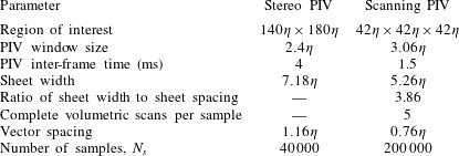
Measurements were performed in a von Kármán mixing tank using both stereoscopic PIV and scanning PIV. The spatial resolution (window sizing) of the scanning and stereo PIV measurements are  $3.06\unicode[STIX]{x1D702}$ and
 $2.04\unicode[STIX]{x1D702}$, respectively, resulting in a vector spacing of
 $0.76\unicode[STIX]{x1D702}$ and
 $1.16\unicode[STIX]{x1D702}$. The sample sizes are 200 000 and 40 000 samples for the scanning and stereo PIV, sampled with a minimum spacing of respectively 2 and 4.5 large eddy turnover times, ensuring statistically independent measurements. Due to technical constraints, the measurement volume for the scanning PIV is limited to
 $42\unicode[STIX]{x1D702}\times 42\unicode[STIX]{x1D702}\times 42\unicode[STIX]{x1D702}$. The stereo PIV measurement covers a larger FOV (
 $154\unicode[STIX]{x1D702}\times 199\unicode[STIX]{x1D702}$), and therefore contributes to an understanding of the larger length scales of the flow.
The stereoscopic PIV data were calibrated and processed using DaVis 8.3, to give two-dimensional three-component (2D3C) velocity fields. The processing involved the application of a multi-pass cross-correlation algorithm with window deformation, and vector validation through application of the RMS criteria over local flow regions. The tomographic scanning PIV algorithm described in Lawson & Dawson (Reference Lawson and Dawson2015) was employed to post-process the volumetric data. In short, the method consists of a laser sheet being traversed (scanned) across a measurement volume at a rate of 250 Hz, while two high speed cameras capture particle images of each illumination. Fifty-four images were captured per scan, and intensity volumes are reconstructed based on the particle images using a multiplicative algebraic reconstruction technique (MART) algorithm. The reconstructed volumes are then cross-correlated to obtain vector fields of velocity. Similarly an in-house multi-pass algorithm with window deformation was used for the cross-correlation, and a correction is applied to correct for the finite sheet speed effects. For each sample, five scans were performed, giving five reconstructed particle volumes and four velocity fields, providing access to acceleration information. A divergence correction is applied to the velocity fields (Wang et al. Reference Wang, Gao, Wei, Li and Wang2017), and a Lagrangian filter similar to Novara & Scarano (Reference Novara and Scarano2013) is then used on the velocity fields to increase the measurement accuracy. In the procedure, artificial tracers inserted to the calculated flow field are tracked backwards and forwards in time, then a second-order polynomial is fitted to these trajectories, where the linear and quadratic terms yield the velocity and the Lagrangian acceleration respectively. As a result, the truncation error and the random error due to the particle positions is reduced. The Lagrangian acceleration fields,  $\text{D}u_{i}/\text{D}t=\unicode[STIX]{x2202}u_{i}/\unicode[STIX]{x2202}t+u_{j}(\unicode[STIX]{x2202}u_{i}/\unicode[STIX]{x2202}x_{j})$, are used to resolve pressure fields using a similar procedure as in Lawson & Dawson (Reference Lawson and Dawson2015). The incompressible Navier–Stokes equation is rearranged to solve for the pressure gradient,
 $\unicode[STIX]{x1D735}p/\unicode[STIX]{x1D70C}=-(\text{D}u_{i}/\text{D}t)+\unicode[STIX]{x1D708}\unicode[STIX]{x1D6FB}^{2}u_{i}$, and when discretised make up an over-determined set of linear equations, which is solved using a least-square fit. However, the artificially inserted particles on the edges of the volume might leave the FOV when tracked in time, and the material derivative at these points will be lost. As a solution to this, the Poisson equation,
 $\unicode[STIX]{x1D6FB}^{2}p/\unicode[STIX]{x1D70C}=-(\unicode[STIX]{x2202}^{2}/\unicode[STIX]{x2202}x_{i}\unicode[STIX]{x2202}x_{j})(u_{i}u_{j})$, is included to the set of linear equations. It should be noted that whenever possible fourth-order central differences are used to estimate first-order derivatives, and fifth-order central differences are used for second-order derivatives.
The volumetric method relies on accurate knowledge of the laser sheet position. The laser sheet position is first calibrated manually. A calibration plate is placed in the measurement volume at various depth positions, then images of the laser sheet itself are acquired while the sheet is traversed across the calibration plate. From these images, laser sheet parameters such as sheet width, spacing, position and orientation are calculated (see Lawson & Dawson (Reference Lawson and Dawson2014) for more details). In addition to this manual calibration, the laser sheet self-calibration method described by Knutsen, Lawson & Worth (Reference Knutsen, Lawson, Dawson and Worth2017) is performed to increase the accuracy of the calibration. This self-calibration is also performed during the experiment to maintain an accurate calibration over long acquisition periods (the data were collected continuously for 12 days), and to be able to detect and correct for potential galvanometer drift.
The scanning PIV technique allows for seeding densities high enough to achieve spatially fully resolved volumetric measurements of the flow for the given Reynolds number,  $Re_{\unicode[STIX]{x1D706}}=199$, which in turn allows us to directly calculate the local dissipation rate, for a flow which is expected to be fully developed (and exhibit an inertial subrange) according to the scaling presented by Dimotakis (Reference Dimotakis2005). The large number of volumetric samples taken combined with the high spatial resolution of the measurements provide well-converged statistics of the complete volumetric and time-dependent flow field without the use of any assumptions. A detailed list of the experimental parameters for the two measurement methods is presented in table 2.
Experimental parameters for both stereo and scanning PIV measurements.

An attempt to evaluate the uncertainty of the data sets has been made through an evaluation of how well the volumetric data obey the divergence-free criteria, and through an estimate of the random measurement error through the correlation function. In addition, where possible an effort has been made to put confidence intervals on certain quantities. See appendix A for more detailed information and results of the evaluation.
2.3 Flow characterisation
The two experimental data sets were taken in the same tank, under the same conditions, but with different measurement techniques. It is therefore useful to classify the similarities and differences between these two data sets, in addition to giving a general characterisation of the flow in this von Kármán mixing tank. This comparison and a more detailed flow characterisation is presented in appendix B. For further flow characteristics, in addition to a comparison with DNS data, see Lawson et al. (Reference Lawson, Bodenschatz, Knutsen, Dawson and Worth2019), which is based on the same scanning PIV data set.
2.3.1 Mean velocity distribution
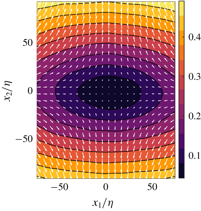
The mean flow can be viewed as a superposition of the two flow modes illustrated in figure 2(b). The mean flow field calculated from the stereo PIV data is shown in figure 3. Contours of normalised velocity magnitude,  $|\boldsymbol{U}|/\langle u_{rms}\rangle$, show that the mean flow in the centre of the tank is of an order of magnitude smaller than the mean fluctuations. The two flow modes resulting in the mean flow are: first, a rotating motion, which rotates in opposite directions at the top and bottom of the tank, creating a shear layer in the mid-plane between the two impellers (Ravelet et al. Reference Ravelet, Marié, Chiffaudel and Daviaud2004; Monchaux et al. Reference Monchaux, Ravelet, Dubrulle, Chiffaudel and Daviaud2006; Cortet et al. Reference Cortet, Diribarne, Monchaux, Chiffaudel, Daviaud and Dubrulle2009); and second, a centrifugal pumping mode, which results in a straining of the flow at the centre of the tank.
Mean flow from the stereo PIV data. Contours represent the magnitude of the mean flow normalised by the mean fluctuations,  $|\boldsymbol{U}|/\langle u_{rms}\rangle$, while the velocity vectors are showing the mean flow in the
 $x_{1}{-}x_{2}$ plane. Every sixth vector is plotted.

The combination of the flow modes results in a stagnation point which occurs approximately at the geometric centre of the tank. The stagnation point in the  $x_{1}{-}x_{2}$ plane for the stereo PIV data is calculated to be at
 $(x_{1,s},x_{2,s})=(5.22\unicode[STIX]{x1D702},-0.1\unicode[STIX]{x1D702})$, while the velocity in the centre of the measurement volume,
 $(x_{1},x_{2})=(0,0)$, is
 $(U_{1},U_{2},U_{3})=(1.7\,\%,0.6\,\%,4.3\,\%)$ of
 $\langle u_{rms}\rangle$. Characteristic for a von Kármán flow, strong gradients are present in all components of the mean flow, with the highest gradient observed in the
 $x_{2}$-direction.
2.4 Calculation of the inter-scale energy budget
The final part of this section is used to present the KHMH equation, which governs the evolution of the trace of the second-order structure function  $\overline{\unicode[STIX]{x1D6FF}q^{2}}(\boldsymbol{x},\boldsymbol{r})\equiv \overline{\unicode[STIX]{x1D6FF}q^{2}(\boldsymbol{x},\boldsymbol{r},t)}=\overline{\unicode[STIX]{x1D6FF}u_{i}(\boldsymbol{x},\boldsymbol{r},t)\unicode[STIX]{x1D6FF}u_{i}(\boldsymbol{x},\boldsymbol{r},t)}$. The KHMH equation is given by (2.8), where for the sake of brevity we do not present the explicit functional dependency of the particular terms:
 $$\begin{eqnarray}\displaystyle & & \displaystyle \!\!\!\frac{\unicode[STIX]{x2202}\overline{\unicode[STIX]{x1D6FF}q^{2}}}{\unicode[STIX]{x2202}t}+\frac{\unicode[STIX]{x2202}}{\unicode[STIX]{x2202}x_{i}}\left(\frac{U_{i}^{+}+U_{i}^{-}}{2}\overline{\unicode[STIX]{x1D6FF}q^{2}}\right)+\frac{\unicode[STIX]{x2202}}{\unicode[STIX]{x2202}r_{i}}\overline{\unicode[STIX]{x1D6FF}u_{i}\unicode[STIX]{x1D6FF}q^{2}}+\frac{\unicode[STIX]{x2202}}{\unicode[STIX]{x2202}r_{i}}\unicode[STIX]{x1D6FF}U_{i}\overline{\unicode[STIX]{x1D6FF}q^{2}}\nonumber\\ \displaystyle & & \displaystyle \!\!\!\quad =-2\overline{\unicode[STIX]{x1D6FF}u_{i}\unicode[STIX]{x1D6FF}u_{j}}\frac{\unicode[STIX]{x2202}}{\unicode[STIX]{x2202}r_{i}}\unicode[STIX]{x1D6FF}U_{j}-\overline{(u_{i}^{+}+u_{i}^{-})\unicode[STIX]{x1D6FF}u_{j}}\frac{\unicode[STIX]{x2202}}{\unicode[STIX]{x2202}x_{i}}\unicode[STIX]{x1D6FF}U_{j}-\frac{\unicode[STIX]{x2202}}{\unicode[STIX]{x2202}x_{i}}\left(\overline{\frac{u_{i}^{+}+u_{i}^{-}}{2}\unicode[STIX]{x1D6FF}q^{2}}\right)\nonumber\\ \displaystyle & & \displaystyle \!\!\!\qquad -\,\frac{2}{\unicode[STIX]{x1D70C}}\frac{\unicode[STIX]{x2202}}{\unicode[STIX]{x2202}x_{i}}\overline{\unicode[STIX]{x1D6FF}u_{i}\unicode[STIX]{x1D6FF}p}+\frac{\unicode[STIX]{x1D708}}{2}\frac{\unicode[STIX]{x2202}^{2}}{\unicode[STIX]{x2202}x_{i}\unicode[STIX]{x2202}x_{i}}\overline{\unicode[STIX]{x1D6FF}q^{2}}+2\unicode[STIX]{x1D708}\frac{\unicode[STIX]{x2202}^{2}}{\unicode[STIX]{x2202}r_{i}\unicode[STIX]{x2202}r_{i}}\overline{\unicode[STIX]{x1D6FF}q^{2}}-4\unicode[STIX]{x1D708}\!\left(\overline{\frac{\unicode[STIX]{x2202}\unicode[STIX]{x1D6FF}u_{j}}{\unicode[STIX]{x2202}x_{i}}\frac{\unicode[STIX]{x2202}\unicode[STIX]{x1D6FF}u_{j}}{\unicode[STIX]{x2202}x_{i}}}+4\overline{\frac{\unicode[STIX]{x2202}\unicode[STIX]{x1D6FF}u_{j}}{\unicode[STIX]{x2202}r_{i}}\frac{\unicode[STIX]{x2202}\unicode[STIX]{x1D6FF}u_{j}}{\unicode[STIX]{x2202}r_{i}}}\right)\!.\quad \!\!\qquad\end{eqnarray}$$
The integral of  $\overline{\unicode[STIX]{x1D6FF}q^{2}}(\boldsymbol{x},\boldsymbol{r})$ over a sphere of a specified radius
 $r=|\boldsymbol{r}|$ can be intuitively understood as
 $1/4$ of the energy accumulated at the scales equal to and smaller than
 $r$ (Davidson Reference Davidson2004). This becomes more apparent when
 $\overline{\unicode[STIX]{x1D6FF}q^{2}}$ is expressed with a Fourier integral, where
 $\boldsymbol{u}(\boldsymbol{x},t)=\iiint _{-\infty }^{\infty }\hat{\boldsymbol{u}}(\unicode[STIX]{x1D73F},t)\exp (\text{i}\unicode[STIX]{x1D73F}\boldsymbol{\cdot }\boldsymbol{x})\,\text{d}\unicode[STIX]{x1D73F}$, which can be written as
 $$\begin{eqnarray}\overline{\unicode[STIX]{x1D6FF}q^{2}}(\boldsymbol{r})=4\iiint _{-\infty }^{\infty }\unicode[STIX]{x1D6F9}(\unicode[STIX]{x1D73F},\boldsymbol{r})\hat{E}(\unicode[STIX]{x1D73F})\,\text{d}\unicode[STIX]{x1D73F},\end{eqnarray}$$
where  $\unicode[STIX]{x1D73F}$ is the wavevector and summation goes over all Fourier modes,
 $\hat{E}$ is the energy associated with
 $\unicode[STIX]{x1D73F}$ and
 $\unicode[STIX]{x1D6F9}=1-\cos (\unicode[STIX]{x1D73F}\boldsymbol{\cdot }\boldsymbol{r})$ can be looked upon as a filter which is weighing the wavenumbers which contribute to
 $\overline{\unicode[STIX]{x1D6FF}q^{2}}(\boldsymbol{x},\boldsymbol{r})$.
Equation (2.8) does not take into account any assumption of homogeneity or isotropy of the flow and thus considers both inter-space and inter-scale transfers of  $\overline{\unicode[STIX]{x1D6FF}q^{2}}$.
Statistics of the studied flow are homogeneous, to a large degree, within the FOV (this was verified for all the particular terms of (2.8)). Therefore, in order to reduce the amount of data as well as for smoothing of our statistics, we shall consider the space-averaged version of (2.8) in all further analysis (note that (2.8) is valid everywhere in the flow field, and thus its space average stays valid as well). The averaging is over the extent of the FOV. Using the same approach as Portela et al. (Reference Portela, Papadakis and Vassilicos2017) and Gomes-Fernandes et al. (Reference Gomes-Fernandes, Ganapathisubramani and Vassilicos2015), the following terms of the space-averaged KHMH equation are identified:
 $$\begin{eqnarray}A_{t}=-A-\unicode[STIX]{x1D6F1}-\unicode[STIX]{x1D6F1}_{U}+{\mathcal{P}}+T_{u}+T_{p}+D_{x}+D_{r}-\unicode[STIX]{x1D716}_{r}\end{eqnarray}$$
and the following meaning can be assigned to them ( $\unicode[STIX]{x2202}{\mathcal{A}}$ and
 $\boldsymbol{n}$ designate the boundary of the FOV and its normal vector, respectively). The spatially averaged unsteady term describes the rate of change in time of the kinetic energy
 $\frac{1}{4}\langle \overline{\unicode[STIX]{x1D6FF}q^{2}}\rangle$ at scale
 $\boldsymbol{r}$:
 $$\begin{eqnarray}A_{t}=A_{t}(\boldsymbol{r},{\mathcal{A}},T)=\frac{1}{4}\left\langle \frac{\unicode[STIX]{x2202}}{\unicode[STIX]{x2202}t}\overline{\unicode[STIX]{x1D6FF}q^{2}(\boldsymbol{x},\boldsymbol{r},t)}\right\rangle =\frac{1}{4}\frac{\unicode[STIX]{x2202}}{\unicode[STIX]{x2202}t}\left\langle \overline{\unicode[STIX]{x1D6FF}q^{2}(\boldsymbol{x},\boldsymbol{r},t)}\right\rangle ;\end{eqnarray}$$
the averaged advection of  $\overline{\unicode[STIX]{x1D6FF}q^{2}}$ through the boundaries of the FOV
 $$\begin{eqnarray}\displaystyle A & = & \displaystyle A(\boldsymbol{r},{\mathcal{A}},T)=\frac{1}{4}\left\langle \frac{\unicode[STIX]{x2202}}{\unicode[STIX]{x2202}x_{i}}\frac{U_{i}^{+}(\boldsymbol{x},\boldsymbol{r})+U_{i}^{-}(\boldsymbol{x},\boldsymbol{r})}{2}\overline{\unicode[STIX]{x1D6FF}q^{2}(\boldsymbol{x},\boldsymbol{r},t)}\right\rangle \nonumber\\ \displaystyle & = & \displaystyle \frac{1}{8|\unicode[STIX]{x2202}{\mathcal{A}}|}\iint _{\unicode[STIX]{x2202}{\mathcal{A}}}(U_{i}^{+}(\boldsymbol{x},\boldsymbol{r})+U_{i}^{-}(\boldsymbol{x},\boldsymbol{r}))\overline{\unicode[STIX]{x1D6FF}q^{2}(\boldsymbol{x},\boldsymbol{r},t)}n_{i}\,\text{d}S;\nonumber\end{eqnarray}$$
the spatially averaged nonlinear inter-scale transfer of  $\overline{\unicode[STIX]{x1D6FF}q^{2}}$ accounting for the effect of nonlinear interactions of scales in redistributing
 $\overline{\unicode[STIX]{x1D6FF}q^{2}}$ in scale space
 $$\begin{eqnarray}\unicode[STIX]{x1D6F1}=\unicode[STIX]{x1D6F1}(\boldsymbol{r},{\mathcal{A}},T)=\frac{1}{4}\left\langle \frac{\unicode[STIX]{x2202}}{\unicode[STIX]{x2202}r_{i}}\overline{\unicode[STIX]{x1D6FF}u_{i}(\boldsymbol{x},\boldsymbol{r},t)\unicode[STIX]{x1D6FF}q^{2}(\boldsymbol{x},\boldsymbol{r},t)}\right\rangle =\frac{1}{4}\frac{\unicode[STIX]{x2202}}{\unicode[STIX]{x2202}r_{i}}\left\langle \overline{\unicode[STIX]{x1D6FF}u_{i}(\boldsymbol{x},\boldsymbol{r},t)\unicode[STIX]{x1D6FF}q^{2}(\boldsymbol{x},\boldsymbol{r},t)}\right\rangle ;\end{eqnarray}$$
the spatially averaged linear equivalent of  $\unicode[STIX]{x1D6F1}$; it accounts for inter-scale transfer of
 $\overline{\unicode[STIX]{x1D6FF}q^{2}}$ by the mean flow
 $$\begin{eqnarray}\unicode[STIX]{x1D6F1}_{U}=\unicode[STIX]{x1D6F1}_{U}(\boldsymbol{r},{\mathcal{A}},T)=\frac{1}{4}\left\langle \frac{\unicode[STIX]{x2202}}{\unicode[STIX]{x2202}r_{i}}\unicode[STIX]{x1D6FF}U_{i}(\boldsymbol{x},\boldsymbol{r})\overline{\unicode[STIX]{x1D6FF}q^{2}(\boldsymbol{x},\boldsymbol{r},t)}\right\rangle =\frac{1}{4}\frac{\unicode[STIX]{x2202}}{\unicode[STIX]{x2202}r_{i}}\left\langle \unicode[STIX]{x1D6FF}U_{i}(\boldsymbol{x},\boldsymbol{r})\overline{\unicode[STIX]{x1D6FF}q^{2}(\boldsymbol{x},\boldsymbol{r},t)}\right\rangle\end{eqnarray}$$
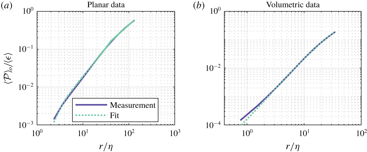
the spatially averaged production of  $\overline{\unicode[STIX]{x1D6FF}q^{2}}$ by the mean flow gradients
 $$\begin{eqnarray}\displaystyle {\mathcal{P}} & = & \displaystyle {\mathcal{P}}(\boldsymbol{r},{\mathcal{A}},T)=-\frac{1}{2}\left\langle \overline{\unicode[STIX]{x1D6FF}u_{i}(\boldsymbol{x},\boldsymbol{r},t)\unicode[STIX]{x1D6FF}u_{j}(\boldsymbol{x},\boldsymbol{r},t)}\frac{\unicode[STIX]{x2202}}{\unicode[STIX]{x2202}r_{i}}\unicode[STIX]{x1D6FF}U_{j}(\boldsymbol{x},\boldsymbol{r})\right\rangle \nonumber\\ \displaystyle & & \displaystyle -\left\langle \overline{(u_{i}^{+}(\boldsymbol{x},\boldsymbol{r},t)+u_{i}^{-}(\boldsymbol{x},\boldsymbol{r},t))\unicode[STIX]{x1D6FF}u_{j}(\boldsymbol{x},\boldsymbol{r},t)}\frac{\unicode[STIX]{x2202}\unicode[STIX]{x1D6FF}}{\unicode[STIX]{x2202}x_{i}}U_{j}(\boldsymbol{x},\boldsymbol{r})\right\rangle ;\nonumber\end{eqnarray}$$
the averaged transport of  $\overline{\unicode[STIX]{x1D6FF}q^{2}}$ by the fluctuating velocity through the boundary of the FOV
 $$\begin{eqnarray}\displaystyle T_{u} & = & \displaystyle T_{u}(\boldsymbol{r},{\mathcal{A}},T)=-\frac{1}{8}\left\langle \frac{\unicode[STIX]{x2202}}{\unicode[STIX]{x2202}x_{i}}\overline{(u_{i}^{+}(\boldsymbol{x},\boldsymbol{r},t)+u_{i}^{-}(\boldsymbol{x},\boldsymbol{r},t))\unicode[STIX]{x1D6FF}q^{2}(\boldsymbol{x},\boldsymbol{r},t)}\right\rangle \nonumber\\ \displaystyle & = & \displaystyle -\frac{1}{8|\unicode[STIX]{x2202}{\mathcal{A}}|}\iint _{\unicode[STIX]{x2202}{\mathcal{A}}}\overline{(u_{i}^{+}(\boldsymbol{x},\boldsymbol{r},t)+u_{i}^{-}(\boldsymbol{x},\boldsymbol{r},t))\unicode[STIX]{x1D6FF}q^{2}(\boldsymbol{x},\boldsymbol{r},t)}n_{i}\,\text{d}S;\nonumber\end{eqnarray}$$
the flux of  $\overline{\unicode[STIX]{x1D6FF}u_{i}\unicode[STIX]{x1D6FF}p}$ through the boundaries of the FOV
 $$\begin{eqnarray}\displaystyle T_{p} & = & \displaystyle T_{p}(\boldsymbol{r},{\mathcal{A}},T)=-\frac{1}{2\unicode[STIX]{x1D70C}}\left\langle \frac{\unicode[STIX]{x2202}}{\unicode[STIX]{x2202}x_{i}}\overline{\unicode[STIX]{x1D6FF}u_{i}(\boldsymbol{x},\boldsymbol{r},t)\unicode[STIX]{x1D6FF}p(\boldsymbol{x},\boldsymbol{r},t)}\right\rangle \nonumber\\ \displaystyle & = & \displaystyle -\frac{1}{2\unicode[STIX]{x1D70C}|\unicode[STIX]{x2202}{\mathcal{A}}|}\iint _{\unicode[STIX]{x2202}{\mathcal{A}}}\overline{\unicode[STIX]{x1D6FF}u_{i}(\boldsymbol{x},\boldsymbol{r},t)\unicode[STIX]{x1D6FF}p(\boldsymbol{x},\boldsymbol{r},t)}n_{i}\,\text{d}S;\nonumber\end{eqnarray}$$
the averaged viscous diffusive flux of  $\overline{\unicode[STIX]{x1D6FF}q^{2}}$ through the boundary of the FOV
 $$\begin{eqnarray}D_{x}=D_{x}(\boldsymbol{r},{\mathcal{A}},T)=\frac{\unicode[STIX]{x1D708}}{8}\left\langle \frac{\unicode[STIX]{x2202}^{2}}{\unicode[STIX]{x2202}x_{i}\unicode[STIX]{x2202}x_{i}}\overline{\unicode[STIX]{x1D6FF}q^{2}(\boldsymbol{x},\boldsymbol{r},t)}\right\rangle =\frac{\unicode[STIX]{x1D708}}{8|\unicode[STIX]{x2202}{\mathcal{A}}|}\iint _{\unicode[STIX]{x2202}{\mathcal{A}}}\frac{\unicode[STIX]{x2202}}{\unicode[STIX]{x2202}x_{i}}\overline{\unicode[STIX]{x1D6FF}q^{2}(\boldsymbol{x},\boldsymbol{r},t)}n_{i}\,\text{d}S;\end{eqnarray}$$
the spatially averaged viscous diffusion of  $\overline{\unicode[STIX]{x1D6FF}q^{2}}$ in scale space
 $$\begin{eqnarray}D_{r}=D_{r}(\boldsymbol{r},{\mathcal{A}},T)=\frac{\unicode[STIX]{x1D708}}{2}\left\langle \frac{\unicode[STIX]{x2202}^{2}}{\unicode[STIX]{x2202}r_{i}\unicode[STIX]{x2202}r_{i}}\overline{\unicode[STIX]{x1D6FF}q^{2}(\boldsymbol{x},\boldsymbol{r},t)}\right\rangle =\frac{\unicode[STIX]{x1D708}}{2}\frac{\unicode[STIX]{x2202}^{2}}{\unicode[STIX]{x2202}r_{i}\unicode[STIX]{x2202}r_{i}}\left\langle \overline{\unicode[STIX]{x1D6FF}q^{2}(\boldsymbol{x},\boldsymbol{r},t)}\right\rangle ;\end{eqnarray}$$
spatially averaged dissipation, which is equivalent to  $\langle \unicode[STIX]{x1D716}\rangle$
 $$\begin{eqnarray}\unicode[STIX]{x1D716}_{r}=\unicode[STIX]{x1D716}_{r}(\boldsymbol{r},{\mathcal{A}},T)=\frac{\unicode[STIX]{x1D708}}{2}\left(\left\langle \overline{\frac{\unicode[STIX]{x2202}u_{j}^{+}(\boldsymbol{x},\boldsymbol{r},t)}{\unicode[STIX]{x2202}x_{i}^{+}}\frac{\unicode[STIX]{x2202}u_{j}^{+}(\boldsymbol{x},\boldsymbol{r},t)}{\unicode[STIX]{x2202}x_{i}^{+}}}\right\rangle +\left\langle \overline{\frac{\unicode[STIX]{x2202}u_{j}^{-}(\boldsymbol{x},\boldsymbol{r},t)}{\unicode[STIX]{x2202}x_{i}^{-}}\frac{\unicode[STIX]{x2202}u_{j}^{-}(\boldsymbol{x},\boldsymbol{r},t)}{\unicode[STIX]{x2202}x_{i}^{-}}}\right\rangle \right)=\langle \unicode[STIX]{x1D716}\rangle .\end{eqnarray}$$
The volumetric data permit direct assessment of all terms in the KHMH equation. However, as each term in the KHMH equation requires derivatives of averaged quantities in all flow directions, it is not possible to calculate them directly from the planar stereo PIV measurements. Therefore, assumptions are required for this data set. Since the flow is assumed to be, on averaged, axisymmetric around the direction  $\hat{\boldsymbol{x}}_{2}$, all the spatial derivatives in the circumferential direction (i.e. along
 $\hat{\boldsymbol{x}}_{3}$ in our present set-up) of averaged flow quantities are expected to vanish and thus are neglected. This assumption allows us to calculate different terms of the KHMH equation, and since the volumetric data are measured under the same flow conditions in the same flow facility, it can be directly tested for the smaller length scales. Further, the unsteady term and the pressure terms are lacking from the stereo PIV data. As the data in this study are collected over a large number of turnover times, it follows from the stationarity assumption that the contribution from the stationary term is expected to go to zero; however, it is a very intermittent quantity which is hard to converge, and its residual value can potentially be of non-negligible order.
3 Inter-scale kinetic energy budget
Having introduced the experimental set-up and methods, we now describe both the distribution of energy across scales, and the transfer of energy in our flow of interest. Our aim is to report the flow behaviour, but also to compare this to other similar investigations. Therefore, we discuss both the scale-space organisation of energy transfer, and the reduced spherically averaged transfer, as well as evaluating this against the classical cascade concept. We finally examine the total inter-scale transfer, and consider which physical phenomena help balance the inter-scale energy budget.
3.1 Second-order structure functions and isotropy
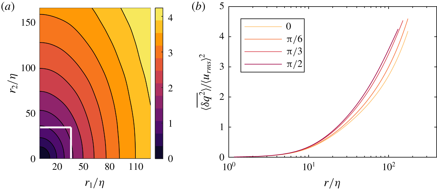
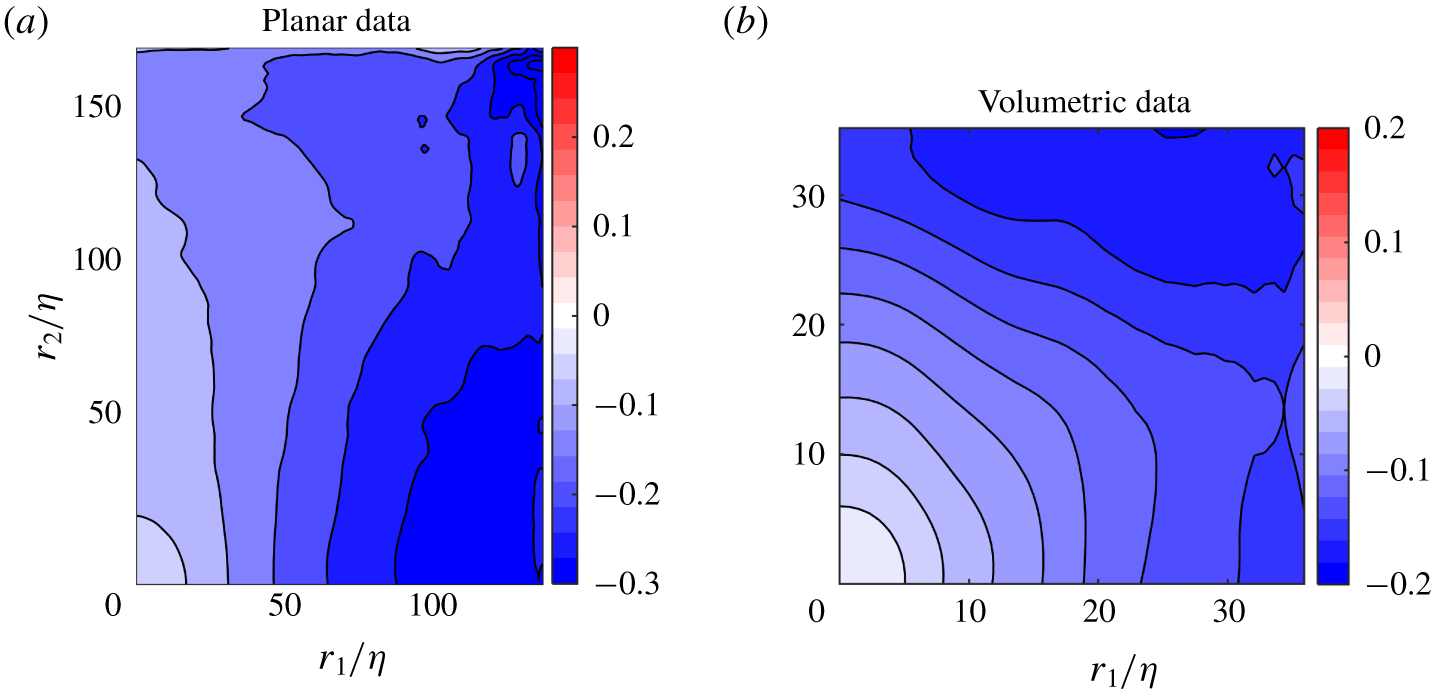
The variation of the normalised combined second-order structure function,  $\langle \overline{\unicode[STIX]{x1D6FF}q^{2}}\rangle /\langle u_{rms}\rangle ^{2}$, with separation distance is shown in figure 4 for the stereo PIV measurements. Figure 4(a) shows the distribution of
 $\langle \overline{\unicode[STIX]{x1D6FF}q^{2}}\rangle$ in the
 $r_{1}{-}r_{2}$-plane, whereas line plots along different angles of
 $\unicode[STIX]{x1D703}$ in the
 $r_{1}{-}r_{2}$-plane is shown in figure 4(b). The non-circular contours in figure 4(a), and the fact that the lines for different values of
 $\unicode[STIX]{x1D703}$ in figure 4(b) do not overlap, show that energy is distributed anisotropically at all scales. The anisotropy is consistent with stronger longitudinal velocity correlations, and therefore lower kinetic energy variations along the symmetry axis of the flow at a given scale. The volumetric measurements from the scanning PIV data (not shown) further shows that
 $\langle \overline{\unicode[STIX]{x1D6FF}q^{2}}\rangle$ is indifferent to rotation around the axis
 $r_{2}$, which resembles the axisymmetry of single-point statistics around the axis of the tank, as discussed earlier.
Distribution of  $\langle \overline{\unicode[STIX]{x1D6FF}q^{2}}\rangle$ normalised by
 $\langle u_{rms}\rangle ^{2}$ from stereo PIV data normalised by
 $\langle u_{rms}\rangle$ from (a) the stereo PIV data, and (b) the scanning PIV data. The different isosurfaces in (b) Line plots of
 $\langle \overline{\unicode[STIX]{x1D6FF}q^{2}}\rangle$ for constant values of
 $\unicode[STIX]{x1D703}=[0,\unicode[STIX]{x03C0}/6,\unicode[STIX]{x03C0}/3,\unicode[STIX]{x03C0}/2]$.

In order to better understand this anisotropic distribution, let us consider a decomposition of  $\langle \overline{\unicode[STIX]{x1D6FF}q^{2}}\rangle (\boldsymbol{r})$ into contributions from velocity components aligned with unit vectors of a spherical coordinate system
 $(r,\unicode[STIX]{x1D703},\unicode[STIX]{x1D719})$ (see figure 1), namely
 $\langle \overline{\unicode[STIX]{x1D6FF}q^{2}}\rangle =\langle \overline{\unicode[STIX]{x1D6FF}u_{i}\unicode[STIX]{x1D6FF}u_{j}}\rangle \cdot (\hat{r}_{i}\hat{r}_{j}+\hat{\unicode[STIX]{x1D703}}_{i}\hat{\unicode[STIX]{x1D703}}_{j}+\hat{\unicode[STIX]{x1D719}}_{i}\hat{\unicode[STIX]{x1D719}}_{j})=\langle \overline{\unicode[STIX]{x1D6FF}u_{r}^{2}}\rangle +\langle \overline{\unicode[STIX]{x1D6FF}u_{\unicode[STIX]{x1D703}}^{2}}\rangle +\langle \overline{\unicode[STIX]{x1D6FF}u_{\unicode[STIX]{x1D719}}^{2}}\rangle$.
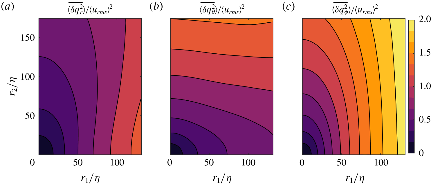
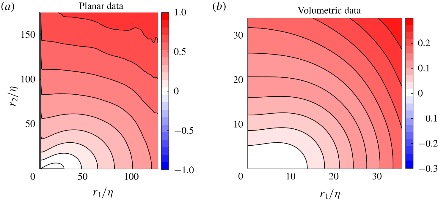
Spherical decomposition of  $\langle \overline{\unicode[STIX]{x1D6FF}q^{2}}\rangle$ from stereo PIV data normalised by
 $\langle u_{rms}\rangle ^{2}$.

Figure 5 shows the individual spherical components of  $\langle \overline{\unicode[STIX]{x1D6FF}q^{2}}\rangle$. To show these over a large range of scales, again the functions are plotted in the
 $r_{1}{-}r_{2}$-plane from the stereo PIV measurements. The figure demonstrates that the main contributions to
 $\langle \overline{\unicode[STIX]{x1D6FF}q^{2}}\rangle$ come from the out of plane component,
 $\langle \overline{\unicode[STIX]{x1D6FF}q_{\unicode[STIX]{x1D719}}^{2}}\rangle$, which is anticipated as this component is parallel to the shear plane and this is where the largest velocity fluctuations exist, and we therefore also expect higher velocity differences. The distribution of
 $\langle \overline{\unicode[STIX]{x1D6FF}q_{\unicode[STIX]{x1D719}}^{2}}\rangle$ also resembles that of
 $\langle \overline{\unicode[STIX]{x1D6FF}q^{2}}\rangle$, with elliptical contour lines stretched in the axial direction. Both the radial and polar parts of
 $\langle \overline{\unicode[STIX]{x1D6FF}q^{2}}\rangle$, shown in figure 5(a,b), are highly anisotropic especially at larger scales, as shown from the visibly non-spherical contour lines. From observing the shape of the contour lines, the terms become more isotropic at smaller scales. The contour lines of the radial part,
 $\langle \overline{\unicode[STIX]{x1D6FF}q_{r}^{2}}\rangle$, are also stretched in
 $r_{2}$-direction in a similar way to the full term
 $\langle \overline{\unicode[STIX]{x1D6FF}q^{2}}\rangle$ and
 $\langle \overline{\unicode[STIX]{x1D6FF}q_{\unicode[STIX]{x1D719}}^{2}}\rangle$, resulting in lower values along the
 $r_{2}$-direction than for the
 $r_{1}$-direction. This is as expected, as the
 $\boldsymbol{r}$-vector is aligned with the shear plane along the
 $r_{1}$-axis, where there are higher fluctuations and thus lower correlations. The azimuthal term exhibits an opposite behaviour, where we observe slightly higher values along the diagonal, and stretched contours in
 $r_{1}$-direction.
To further quantify the level of isotropy and how this varies with scale and for the different components, let us define a measure of isotropy of an arbitrary function  $f(\boldsymbol{r})$ at a given scale
 $r$ designated as
 $\unicode[STIX]{x1D70E}_{f}(r)$:
 $$\begin{eqnarray}\unicode[STIX]{x1D70E}_{f}(r)=\frac{1}{\langle f(\boldsymbol{r})\rangle _{\circ }}\sqrt{\langle (f(\boldsymbol{r})-\langle f(\boldsymbol{r})\rangle _{r})^{2}\rangle _{\circ }}.\end{eqnarray}$$
Note that the above definition is equivalent to considering the  $L_{2}$ norm of coefficients in a spherical harmonics decomposition (Arad, L’vov & Procaccia Reference Arad, L’vov and Procaccia1999; Kurien et al. Reference Kurien, L’vov, Itamar and Sreenivasan2000).
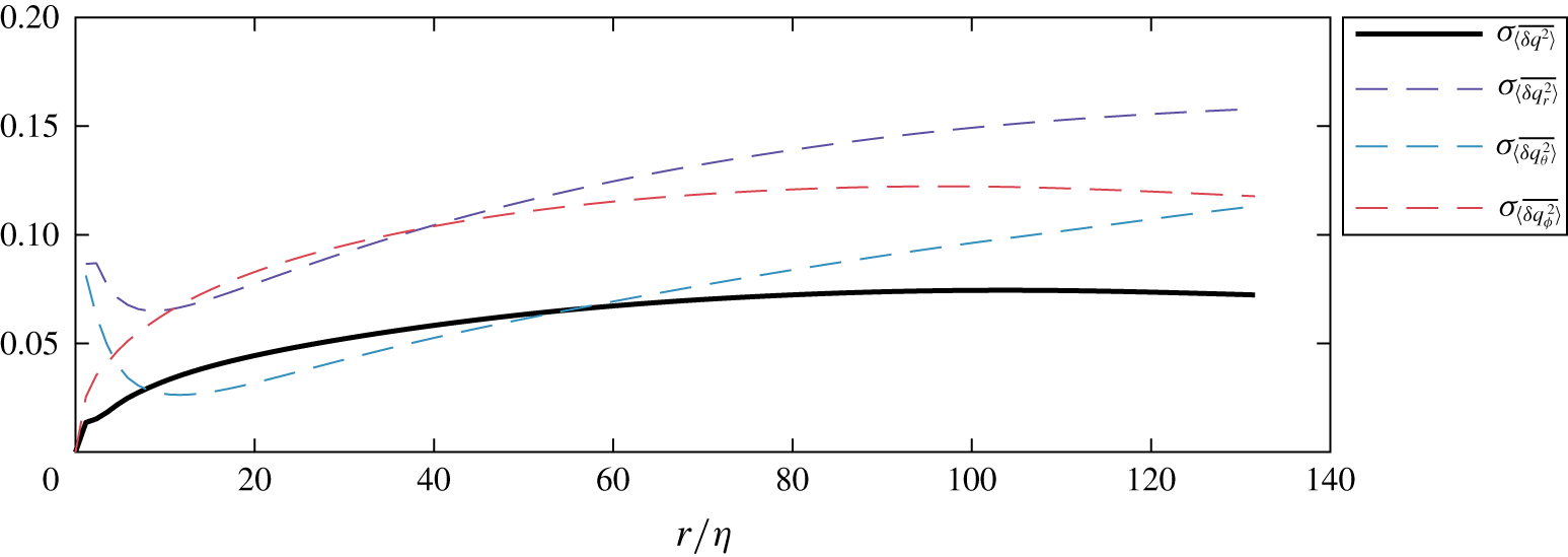
If  $\langle \overline{\unicode[STIX]{x1D6FF}q^{2}}\rangle$ was distributed isotropically, this parameter would take a constant value of zero. The results demonstrate that the standard deviation of the contour lines along constant
 $\langle \overline{\unicode[STIX]{x1D6FF}q^{2}}\rangle$ is never zero, and that deviations in
 $\langle \overline{\unicode[STIX]{x1D6FF}q^{2}}\rangle$ along a constant radius, representing the level of anisotropy, increase with separation distance until
 $r\approx 60\unicode[STIX]{x1D702}\approx 0.33L_{LL}$, where the curve flattens out before it starts to slightly decrease at
 $r\approx 100\unicode[STIX]{x1D702}\approx 0.55L_{LL}$. From
 $r=60\unicode[STIX]{x1D702}$ to
 $r=130\unicode[STIX]{x1D702}$, the value of
 $\unicode[STIX]{x1D70E}_{\langle \overline{\unicode[STIX]{x1D6FF}q^{2}}\rangle }$ is constant to within 10 % of its maximum value. One would expect increasing anisotropy for larger scales, but studying figure 6, it is clear that also
 $\langle \overline{\unicode[STIX]{x1D6FF}q_{\unicode[STIX]{x1D719}}^{2}}\rangle$ shows the same tendency to plateau within the FOV. The plateau behaviour and the slight decrease in anisotropy of both
 $\langle \overline{\unicode[STIX]{x1D6FF}q^{2}}\rangle$ and
 $\langle \overline{\unicode[STIX]{x1D6FF}q_{r}^{2}}\rangle$ may be caused by the increasing importance of
 $\langle \overline{\unicode[STIX]{x1D6FF}q_{\unicode[STIX]{x1D703}}^{2}}\rangle$. From figure 5(b) it is clear that the contour lines of
 $\langle \overline{\unicode[STIX]{x1D6FF}q_{\unicode[STIX]{x1D703}}^{2}}\rangle$ are elongated in the
 $r_{1}$-direction while the other two terms are elongated in the
 $r_{2}$-direction, especially for larger values of
 $r$, and thus making the final term
 $\langle \overline{\unicode[STIX]{x1D6FF}q^{2}}\rangle$ more isotropic than its components, i.e. different RMS values for different velocity components.
Isotropy metric  $\unicode[STIX]{x1D70E}$ of
 $\langle \overline{\unicode[STIX]{x1D6FF}q^{2}}\rangle$ and its spherical components.

Figure 6 shows that while the distribution of  $\langle \overline{\unicode[STIX]{x1D6FF}q^{2}}\rangle$ is anisotropic at all scales, the level of anisotropy is highest for
 $r\approx 100\unicode[STIX]{x1D702}$. If the anisotropy is driven by the shear layer between the counter-rotating fluid cells, it is expected to increase with distance from the axis of symmetry following the shear. However, the plateau in the level of anisotropy results from the balance between the increments of the different velocity components. The terms
 $\langle \overline{\unicode[STIX]{x1D6FF}q_{r}^{2}}\rangle$ and
 $\langle \overline{\unicode[STIX]{x1D6FF}q_{\unicode[STIX]{x1D703}}^{2}}\rangle$ are anisotropic even at very small scales, which is a result of the apparent anisotropy of single-point velocity statistics. However, there are initial decreases of anisotropy of both terms (with minima respectively at
 $7\unicode[STIX]{x1D702}$ and
 $10\unicode[STIX]{x1D702}$), followed by the subsequent growths. This behaviour, although surprising, might be the result of specific relations between directional Taylor microscales, directional integral length scales and variances of particular velocity components.
A more thorough investigation of  $\langle \overline{\unicode[STIX]{x1D6FF}q_{r}^{2}}\rangle$ is motivated by the highly anisotropic distribution of the term. Figure 7 demonstrates the orientation dependency of
 $\langle \overline{\unicode[STIX]{x1D6FF}q^{2}}\rangle$ through a line plot in (a), where the value of the term is plotted at different values of polar coordinate
 $\unicode[STIX]{x1D703}$, and in (b) where the full distribution of the term is shown.
 $\langle \overline{\unicode[STIX]{x1D6FF}q_{r}^{2}}\rangle$ is the longitudinal second-order structure function, which for homogeneous isotropic turbulence is related to the dissipation rate through Kolmogorov’s
 $2/3\text{rds}$ law
 $$\begin{eqnarray}\overline{\unicode[STIX]{x1D6FF}u_{r}^{2}}(\boldsymbol{r})=C_{2}\unicode[STIX]{x1D716}^{2/3}|\boldsymbol{r}|^{2/3},\end{eqnarray}$$
where  $C_{2}$ is a constant which is expected to be universal (Pope Reference Pope2005). In the present study a value of
 $C_{2}=2.1$ is found from the spherical average of
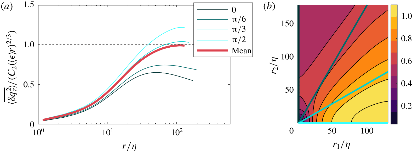
 $\langle \overline{\unicode[STIX]{x1D6FF}u_{r}^{2}}\rangle _{\circ }(r)$, shown in the inset in figure 7(a), which is consistent with previous studies (Ni & Xia Reference Ni and Xia2013).
Orientational variation of  $\langle \overline{\unicode[STIX]{x1D6FF}q_{r}^{2}}\rangle$ normalised. (a) Along fixed values of
 $\unicode[STIX]{x1D703}$, where the inset shows the spherical mean value. (b) Contour plot of
 $\langle \overline{\unicode[STIX]{x1D6FF}q_{r}^{2}}\rangle /(C_{2}(\langle \unicode[STIX]{x1D716}\rangle r)^{2/3})$. Lines from (a) marked in (b).

Figure 7 shows the normalised  $\langle \overline{\unicode[STIX]{x1D6FF}q_{r}^{2}}\rangle$, which is expected to have a constant value in the inertial range, and for most orientations, the term has reached a plateau. The plateau has, however, a different value for different orientations. This directional dependency indicates that, depending on along which orientation we calculate the second order longitudinal structure function, the resulting dissipation rate would vary significantly if a constant value of
 $C_{2}$ is used. This result is in contrast to the findings in Chang, Bewley & Bodenschatz (Reference Chang, Bewley and Bodenschatz2012), where they study an anisotropic, zero shear flow, and conclude that
 $C_{2}$ shows no dependency on isotropy. This indicates that the mean flow gradients in the von Kármán flow cause the directional dependency of
 $C_{2}$, which is consistent with the predictions in Lumley (Reference Lumley1967), which are discussed in § 3.4 in Biferale & Procaccia (Reference Biferale and Procaccia2005). The term also levels off at different values for
 $r$, indicating that the onset of the inertial range is also dependent on orientation in scale space. This is consistent with the anisotropy we observe at small scales.
3.2 Energy transfer and isotropy
After establishing the scale-space distribution of energy, it is now of interest to examine both the magnitude and direction of energy transfer. This is presented through the flux of  $\langle \overline{\unicode[STIX]{x1D6FF}q^{2}}\rangle$ in scale space,
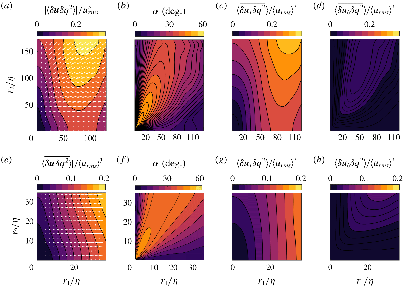
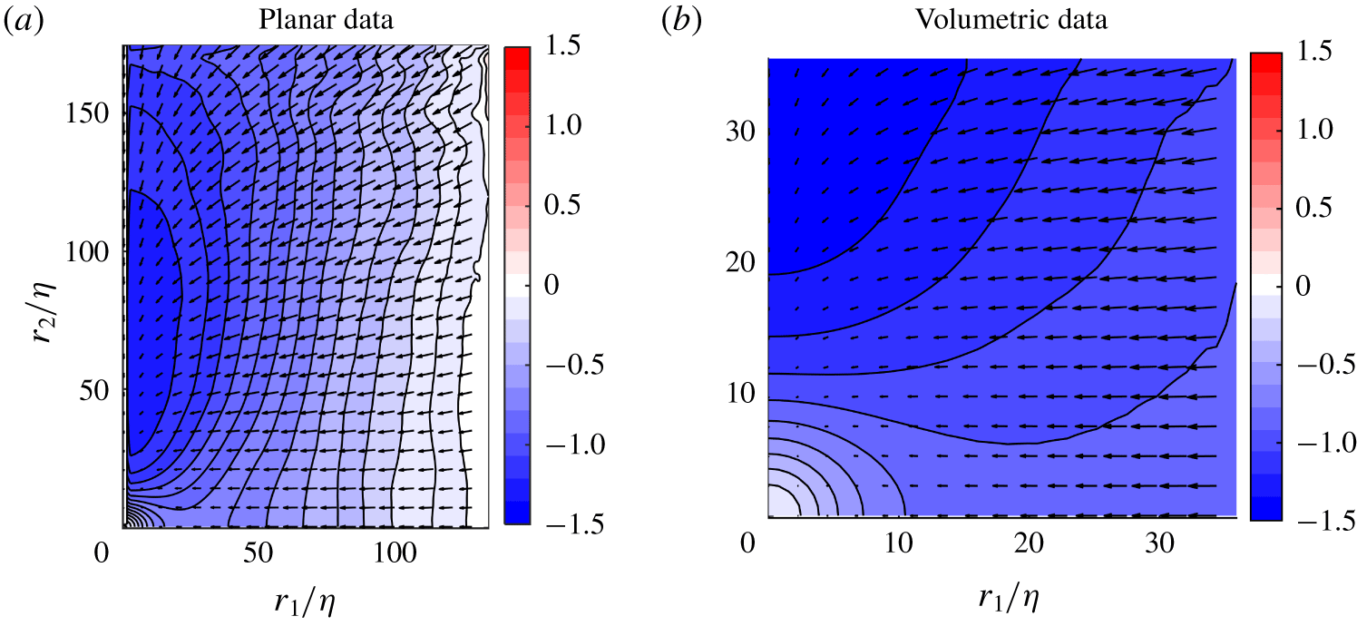
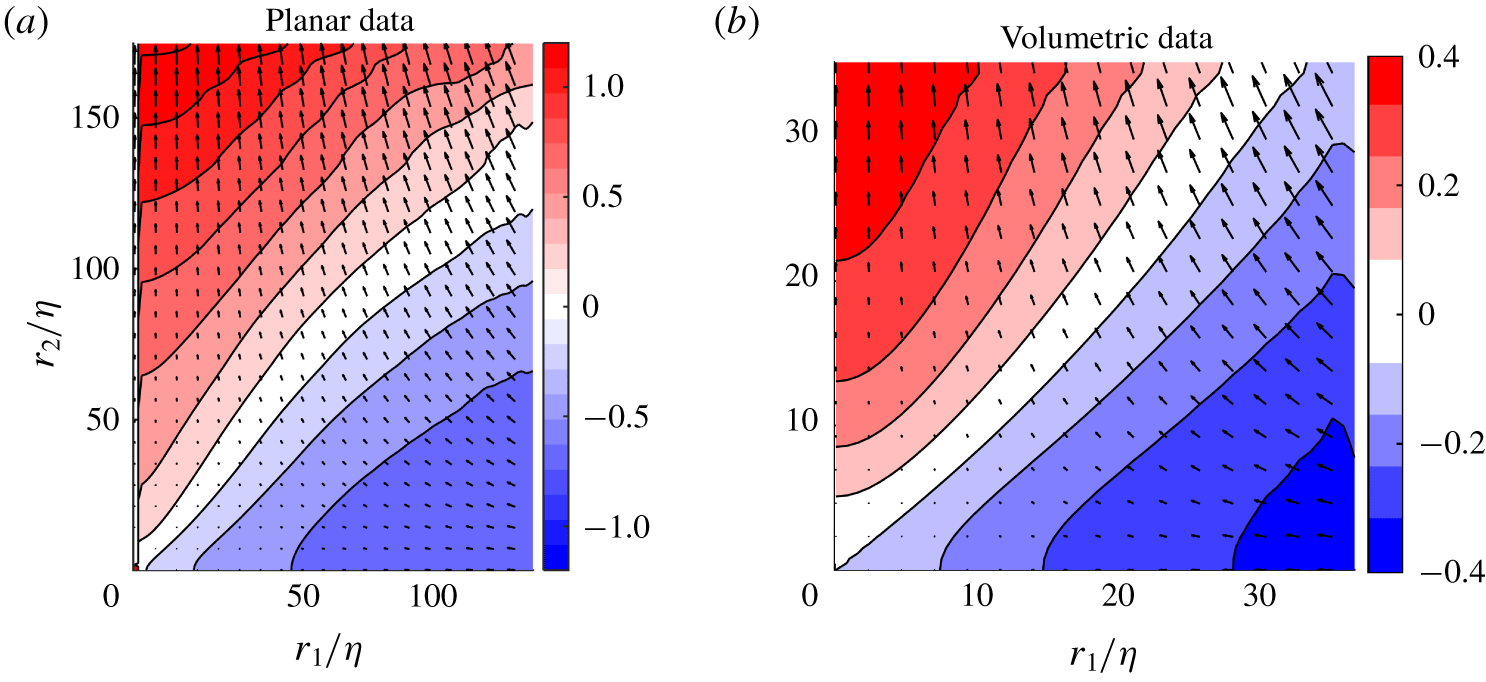
 $\langle \overline{\unicode[STIX]{x1D6FF}\boldsymbol{u}\unicode[STIX]{x1D6FF}q^{2}}\rangle$, which is shown in figures 8(a) and 8(d) for the stereo and scanning PIV data, respectively. While the discussion relates mainly to the planar data which cover a wider range of scales, good agreement is consistently observed at smaller scales for the volumetric data. Here the contours represent the flux magnitude, and the quiver arrows indicate the vector orientation which represents the scale-space direction of the energy transfer. As separation distance increases so does the magnitude of the energy transfer, and therefore energy transfer takes place primarily at larger scales. There is, however, a significant level of anisotropy shown at all scales, with a non-uniform preference for transfer at horizontal and vertical scales, shown by the peak magnitude, which is observed at a scale-space location of
 $(r_{1}/\unicode[STIX]{x1D702},r_{2}/\unicode[STIX]{x1D702})\approx (100,150)$.
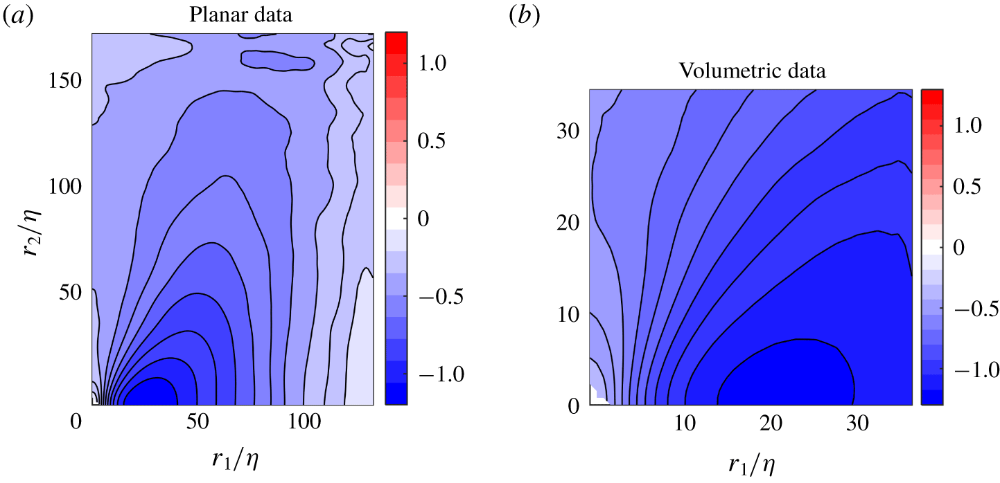
(a,e) Distribution of magnitude of  $\langle \unicode[STIX]{x1D6FF}\overline{\boldsymbol{u}\unicode[STIX]{x1D6FF}q^{2}}\rangle$ with quiver arrows indicating the orientation of the vector
 $\langle \overline{\unicode[STIX]{x1D6FF}\boldsymbol{u}\unicode[STIX]{x1D6FF}q^{2}}\rangle$. For better visibility, only every eighth vector from the stereo planar data and every fourth vector from the volumetric data are plotted. (b,f) Deviation angle, the angle between radial vector
 $\boldsymbol{r}$ pointing towards the origin and
 $\langle \overline{\unicode[STIX]{x1D6FF}\boldsymbol{u}\unicode[STIX]{x1D6FF}q^{2}}\rangle$. (c,g) Radial part of third-order structure function,
 $\langle \overline{\unicode[STIX]{x1D6FF}u_{r}\unicode[STIX]{x1D6FF}q^{2}}\rangle$ (positive direction is set parallel to
 $\boldsymbol{r}$). (d,h) Tangential part of third-order structure function,
 $\langle \overline{\unicode[STIX]{x1D6FF}u_{\unicode[STIX]{x1D703}}\unicode[STIX]{x1D6FF}q^{2}}\rangle$. (a–d) From stereo PIV data, while (e–h) are from scanning PIV data.

It is interesting to consider this distribution together with the direction of the energy transfer. The quiver arrows describe the redistribution of  $\langle \overline{\unicode[STIX]{x1D6FF}q^{2}}\rangle$ in scale space. A purely radial vector distribution pointing towards the origin
 $(r_{1},r_{2})=(0,0)$ would mean energy was being transferred directly from larger to smaller scales. This radial part of the energy flux is hereafter represented by
 $\langle \overline{\unicode[STIX]{x1D6FF}u_{r}\unicode[STIX]{x1D6FF}q^{2}}\rangle \equiv \langle \overline{\unicode[STIX]{x1D6FF}\boldsymbol{u}\unicode[STIX]{x1D6FF}q^{2}}\rangle \boldsymbol{\cdot }\hat{\boldsymbol{r}}$. It is, however, clear that the orientation of the vectors are rarely purely radial. Whenever
 $|\langle \overline{\unicode[STIX]{x1D6FF}\boldsymbol{u}\unicode[STIX]{x1D6FF}q^{2}}\rangle |$ and
 $\langle \overline{\unicode[STIX]{x1D6FF}u_{r}\unicode[STIX]{x1D6FF}q^{2}}\rangle$ are not the same, there is also a redistribution of
 $\langle \overline{\unicode[STIX]{x1D6FF}q^{2}}\rangle$ at the given scale
 $r$ from one orientation to another, and energy is not purely transferred across scales.
The amount of scale to scale transfer and redistribution is indicated through the vectors in figure 8(a,e), and is made more explicit through the calculation of the angle between  $\langle \overline{\unicode[STIX]{x1D6FF}\boldsymbol{u}\unicode[STIX]{x1D6FF}q^{2}}\rangle$ and the radial vector,
 $\boldsymbol{r}$, which is denoted,
 $\unicode[STIX]{x1D6FC}$, and plotted in figure 8(b,f). These figures show that along the horizontal and vertical axes, where
 $r_{2}\ll \unicode[STIX]{x1D702}$ and
 $r_{1}\ll \unicode[STIX]{x1D702}$ respectively, the angle
 $\unicode[STIX]{x1D6FC}\approx 0^{\circ }$, and therefore the energy is only transferred down scale without redistribution. While the magnitude along the vertical axis is relatively small, the magnitude is more significant along the horizontal axis indicating a reasonable level of energy transfer along this path. Alternatively, away from the horizontal and vertical axes it appears that at the majority of scales, a combination of downscale energy transfer and redistribution within certain scales coexist, evidenced through non-zero values of
 $\unicode[STIX]{x1D6FC}$ within a range of
 $0^{\circ }$–
 $60^{\circ }$. The positive distribution of the angle arises due to the combination of radial and horizontal components, meaning there is often a significant component of the flux pointing toward the symmetry axis. This implies energy is redistributed to structures which are orientated such that they result in higher velocity correlations in the vertical direction in comparison with the horizontal direction, before being transported down the scales. This redistribution of energy therefore mirrors the behaviour of the mean velocity field and may therefore be directly related to the axially straining of the flow field which exists at the centre of the flow.
To clarify this still further it is possible to isolate the downscale transfer of energy from the total energy transfer. To this end figures 8(c) and 8(g) shows the radial component of the third-order structure function,  $\langle \overline{\unicode[STIX]{x1D6FF}u_{r}\unicode[STIX]{x1D6FF}q^{2}}\rangle$, where the positive direction is defined away from the origin. For comparison, the tangential component,
 $\langle \overline{\unicode[STIX]{x1D6FF}u_{\unicode[STIX]{x1D703}}\unicode[STIX]{x1D6FF}q^{2}}\rangle \equiv \hat{\unicode[STIX]{x1D73D}}\boldsymbol{\cdot }\langle \overline{\unicode[STIX]{x1D6FF}\boldsymbol{u}\unicode[STIX]{x1D6FF}q^{2}}\rangle$, is also included in figures 8(d) and 8(h). From the figures, it is clear that the radial component dominates the transfer.
 $\langle \overline{\unicode[STIX]{x1D6FF}u_{r}\unicode[STIX]{x1D6FF}q^{2}}\rangle$ shows a strong orientation dependence, which is very similar in terms of its distribution to the magnitude of
 $\langle \overline{\unicode[STIX]{x1D6FF}\boldsymbol{u}\unicode[STIX]{x1D6FF}q^{2}}\rangle$. Therefore, this shows that despite a certain amount of energy redistribution at some scales the majority of the energy is transferred downscale. The characteristic non-spherical distribution of this downscale transfer, however, shows that this transfer occurs anisotropically, with structures with higher velocity increments in the
 $r_{1}$-orientation dominating the transfer. This preferential transfer of energy at different scale-space orientations represents a departure from the straightforward concept of isotropic downscale energy transfer. These distributions of energy transfer also show significant differences from those obtained in nominally isotropic cases (Lamriben, Cortet & Moisy Reference Lamriben, Cortet and Moisy2011; Carter & Coletti Reference Carter and Coletti2018), raising the possibility that the large-scale flow continues to exert an influence even at small scales.
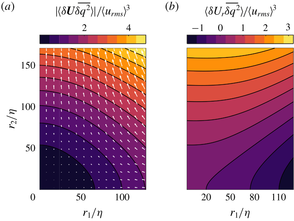
(a) Distribution of magnitude of  $\langle \unicode[STIX]{x1D6FF}\boldsymbol{U}\overline{\unicode[STIX]{x1D6FF}q^{2}}\rangle$ with quiver arrows indicating the orientation of the vector
 $\langle \unicode[STIX]{x1D6FF}\boldsymbol{U}\overline{\unicode[STIX]{x1D6FF}q^{2}}\rangle$ normalised by
 $\langle u_{rms}\rangle ^{3}$. For better visibility only every eighth vector is plotted. (b) Distribution of radial flux
 $\langle \overline{\unicode[STIX]{x1D6FF}q^{2}}\rangle$ by mean flow,
 $\langle \unicode[STIX]{x1D6FF}\boldsymbol{U}\overline{\unicode[STIX]{x1D6FF}q^{2}}\rangle$.

Despite the small magnitude of the mean flow relative to the turbulent fluctuations, it is also interesting to examine its role in the transfer of  $\langle \overline{\unicode[STIX]{x1D6FF}q^{2}}\rangle$. Therefore, the magnitude of the flux of
 $\langle \overline{\unicode[STIX]{x1D6FF}q^{2}}\rangle$ in scale space by the mean flow,
 $|\langle \unicode[STIX]{x1D6FF}\boldsymbol{U}\overline{\unicode[STIX]{x1D6FF}q^{2}}\rangle |$, is shown in figure 9(a). The magnitude and orientation of the flux follow the mean flow distribution, increasing in magnitude with separation distance,
 $r$. However, perhaps surprisingly, the magnitude of this flux is of an order of magnitude larger than the flux of
 $\langle \overline{\unicode[STIX]{x1D6FF}\boldsymbol{u}\unicode[STIX]{x1D6FF}q^{2}}\rangle$ by the turbulent fluctuations. This is a result of the strong spatial mean flow gradients, and the mean stagnation flow pattern characteristic of this configuration, which result in significant mean velocity differences for intermediate separation distances due to the inhomogeneity of the mean flow despite its relatively low magnitude.
In terms of directionality, the vector arrows are negative in the  $r_{1}$-direction indicating downscale transport of energy along this axis, while they are positive in the
 $r_{2}$-direction, resulting in a transfer of energy up the scales along this axis. This balance is made more explicit in figure 9(b), which shows the radial component of this term,
 $\langle \unicode[STIX]{x1D6FF}U_{r}\overline{\unicode[STIX]{x1D6FF}q^{2}}\rangle \equiv \langle \unicode[STIX]{x1D6FF}\boldsymbol{U}\overline{\unicode[STIX]{x1D6FF}q^{2}}\rangle \boldsymbol{\cdot }\hat{\boldsymbol{r}}$. The positive and negatively signed regions indicate a net transfer of energy by the mean flow downscale for angles
 $50^{\circ }<\unicode[STIX]{x1D703}<90^{\circ }$, and upscale for
 $0^{\circ }<\unicode[STIX]{x1D703}<50^{\circ }$. Even excluding scale to scale redistribution, the magnitude of the energy transfer is still significantly larger than that of the turbulent fluctuations. Therefore, despite the small relative magnitude of the mean flow at the centre of a von Kármán tank, this dominates the scale to scale energy transfer. Therefore, in contrast to previous investigations in which the mean flow contribution is negligible (Campagne et al. Reference Campagne, Gallet, Moisy and Cortet2014; Gomes-Fernandes et al. Reference Gomes-Fernandes, Ganapathisubramani and Vassilicos2015; Valente & Vassilicos Reference Valente and Vassilicos2015; Carter & Coletti Reference Carter and Coletti2018), the role of the mean flow cannot be neglected in the present work and will be further examined in the following sections.
3.3 Application of the spherically averaged KHMH equation
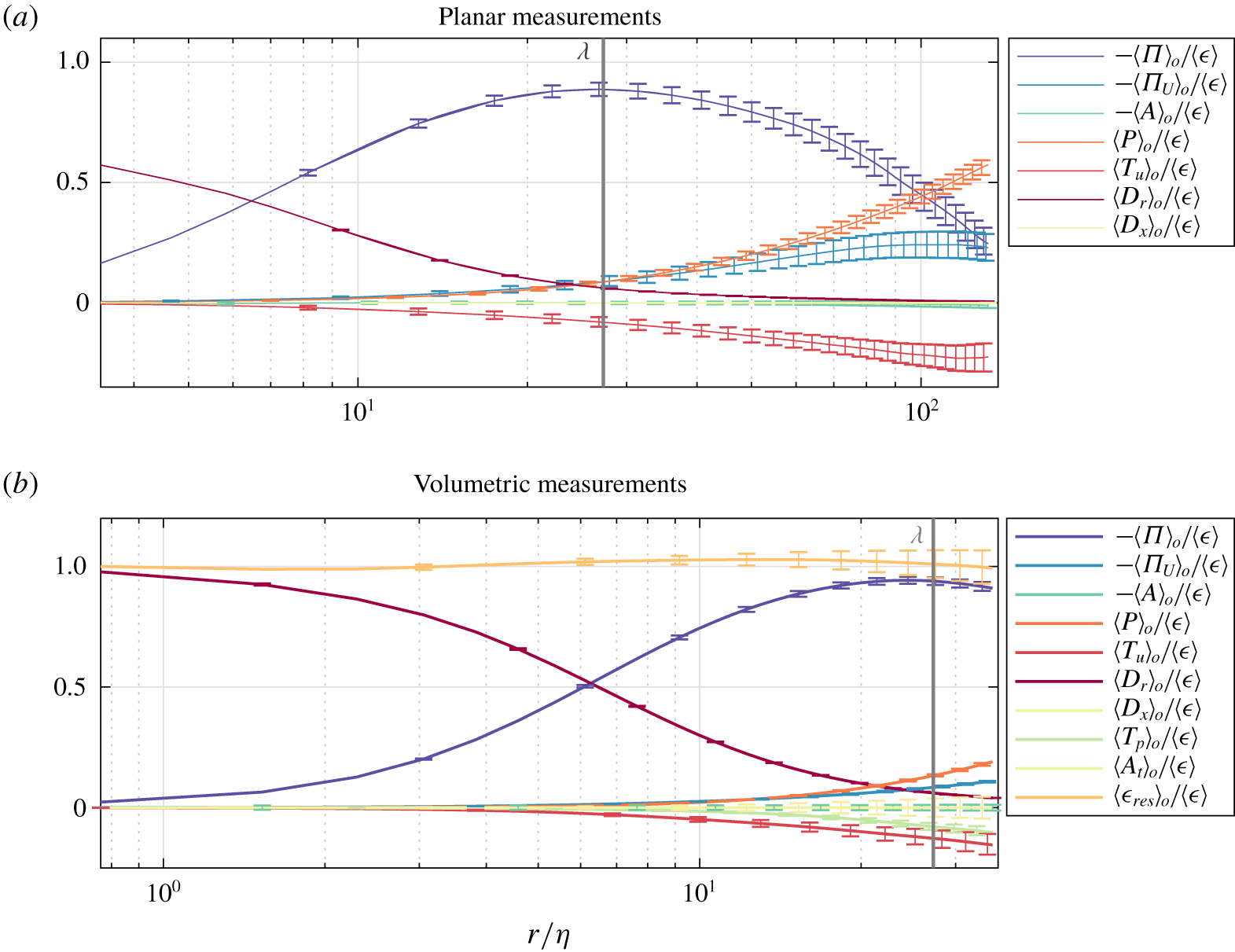
In order to understand the evolution of the energy distribution we now begin to examine the KHMH equation. It is again an advantage to use both the planar data for the larger FOV and the volumetric data, both to be able to validate the planar data at small length scales, and to have direct access to all terms in the KHMH equation without the use of assumptions. In order to determine which contributions play the most significant role in the inter-scale energy transfer in terms of magnitude we begin by analysing their spherical averages, which are shown in figure 10, with each term normalised by  $\langle \unicode[STIX]{x1D716}\rangle$. The 95 % confidence intervals are calculated as described in appendix A. The width of the confidence intervals increase with separation distance as expected, due to the reduction in available samples for higher separations. The greatest uncertainties were calculated for the stereo PIV data and the scanning PIV data, with a value of 5.8 % of
 $\langle \unicode[STIX]{x1D716}\rangle$ for
 $\langle T_{u}\rangle _{\circ }$, and 4.6 % of
 $\langle \unicode[STIX]{x1D716}\rangle$ for
 $\langle A_{t}\rangle _{\circ }$, respectively. This low level of uncertainty results from the extremely large size of the data sets.
Spherically averaged terms of the KHMH equation for the planar and volumetric measurements, where the subscript  $\circ$ indicates spherical mean values. The Taylor microscale
 $\unicode[STIX]{x1D706}$ is marked.

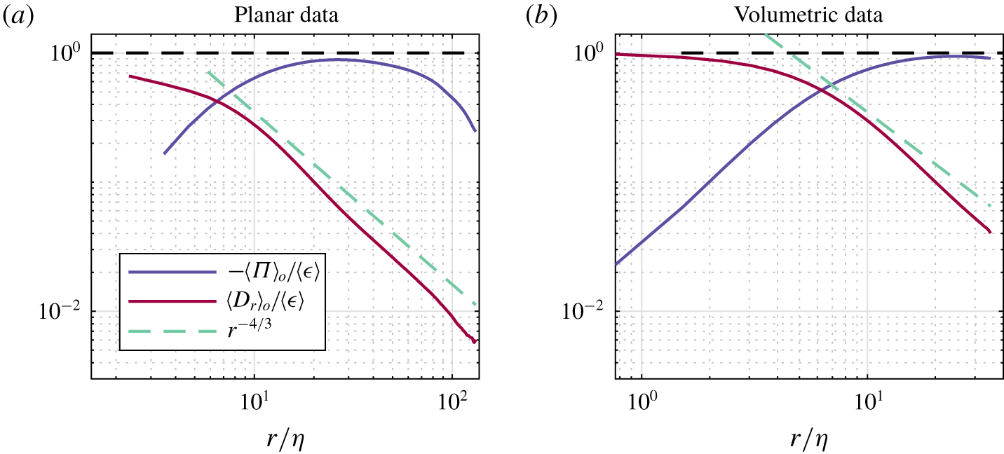
Examining initially the planar data described in figure 10(a), up to intermediate scales  $(r<90\unicode[STIX]{x1D702})$ it is clear that the budget is dominated by nonlinear transfer,
 $\langle \unicode[STIX]{x1D6F1}\rangle _{\circ }$, and the viscous diffusion diffusion term,
 $\langle D_{r}\rangle _{\circ }$, with the other terms only becoming significant at larger scales. As the viscous diffusion terms only contribute at very low separation distances, where the viscous forces are significant
 $(r/\unicode[STIX]{x1D702}\ll 25)$, within the range
 $6\unicode[STIX]{x1D702}<r<90\unicode[STIX]{x1D702}$ the energy transfer is therefore defined primarily by the nonlinear term. This balance is confirmed by the volumetric measurements shown in figure 10(b), which show a very similar distribution of terms over the restricted range of scales available to this technique. Given that the residual dissipation rate
 $\unicode[STIX]{x1D716}_{res}=A_{t}+A+\unicode[STIX]{x1D6F1}+\unicode[STIX]{x1D6F1}_{U}-{\mathcal{P}}-T_{u}-T_{p}-D_{x}-D_{r}$ normalised with the directly evaluated dissipation, i.e.
 $\unicode[STIX]{x1D716}_{res}/\langle \unicode[STIX]{x1D716}\rangle$, should have a constant value of 1, the volumetric measurements demonstrate the energy transfer budget is well captured, with a maximum residual deviation of 2.9 %. Therefore, it can be stated that
 $\unicode[STIX]{x1D716}_{res}/\langle \unicode[STIX]{x1D716}\rangle =1$ within the uncertainty of the measurements. This is an important test that is only possible to make with the volumetric time resolved measurements, which allow the unsteady,
 $A_{t}$, and pressure,
 $T_{p}$, terms to be directly quantified.
The instantaneous value of the nonlinear inter-scale energy transfer,  $(\unicode[STIX]{x2202}/\unicode[STIX]{x2202}r_{i})\unicode[STIX]{x1D6FF}u_{i}\unicode[STIX]{x1D6FF}q^{2}$ fluctuates dramatically, from highly positive to highly negative values, in accordance with the results from Debue et al. (Reference Debue, Shukla, Kuzzay, Faranda, Saw, Daviaud and Dubrulle2018b), and it is only when considering its mean value over time that
 $(\unicode[STIX]{x2202}/\unicode[STIX]{x2202}r_{i})\overline{\unicode[STIX]{x1D6FF}u_{i}\unicode[STIX]{x1D6FF}q^{2}}$ is positive. It is of particular interest to consider the magnitude of
 $\langle \unicode[STIX]{x1D6F1}\rangle _{\circ }$ in terms of Kolmogorov’s hypothesis of local equilibrium, where it is assumed that this term should equal the dissipation rate in the inertial range of scales,
 $\unicode[STIX]{x1D6F1}=-\unicode[STIX]{x1D716}$. From the planar data
 $\unicode[STIX]{x1D6F1}$ does not reach a plateau, but instead increases rapidly at small scales before reaching a maximum value of
 $-0.89\langle \unicode[STIX]{x1D716}\rangle$ at a scale
 ${\approx}\unicode[STIX]{x1D706}$, and then decreases slowly with increasing length scale. Therefore, the prediction
 $\langle \unicode[STIX]{x1D6F1}\rangle _{\circ }\approx -\langle \unicode[STIX]{x1D716}\rangle$ is quite reasonable around
 $r=\unicode[STIX]{x1D706}$. In this case the underlying reason for the success of this prediction then is the small magnitude of the remaining spherically averaged terms in the KHMH equation, combined with the mixed sign of these which act to cancel each other out to some degree.
The terms  $A$ and
 $T_{u}$ from the KHMH equation represent transport of
 $\langle \unicode[STIX]{x1D6FF}q^{2}\rangle$ in physical space by the mean flow and the fluctuations, respectively. When integrated over all separations
 $r$, these terms can be compared with the findings of Marié & Daviaud (Reference Marié and Daviaud2004) who investigated the importance of the mean flow and the turbulent fluctuations in the angular momentum budget in physical space in a von Kármán flow. From the current study, we see that
 $\langle A\rangle _{\circ }$ is zero for all separations both from the volumetric and the planar measurements, whereas
 $\langle T_{u}\rangle _{\circ }$ has a non-zero value, and will thus dominate the transfer of
 $\langle \overline{\unicode[STIX]{x1D6FF}q^{2}}\rangle$ in physical space. The significance of the mean flow and the fluctuations for the transport of
 $\langle \overline{\unicode[STIX]{x1D6FF}q^{2}}\rangle$ in the centre of the tank is therefore comparable to the transport of momentum found in Marié & Daviaud (Reference Marié and Daviaud2004). Further,
 $\langle D_{x}\rangle _{\circ }$, which is negligible at all scales accessible in the current study, can be compared to the viscous term studied in Marié & Daviaud (Reference Marié and Daviaud2004) (equation (3)), which was reported to have a small overall contribution.
It is also worth observing that the Taylor microscale appears to reasonably define the transition between viscous and inertial ranges based on the decreasing significance of  $\langle D_{r}\rangle _{\circ }$ and the increasing significance of
 $\langle \unicode[STIX]{x1D6F1}\rangle _{\circ }$, which is in agreement with Valente & Vassilicos (Reference Valente and Vassilicos2015), where they prove that
 $\langle D_{r}\rangle _{\circ }$ is only significant at scales smaller than
 $\unicode[STIX]{x1D706}$. This might, however, be a coincidence as this coincides with the conventional beginning of the inertial range at
 $r\approx 30\unicode[STIX]{x1D702}$ (Pope Reference Pope2005). The behaviour of
 $\langle D_{r}\rangle _{\circ }$ has earlier been predicted (Dubrulle Reference Dubrulle2019) and shown (Debue et al. Reference Debue, Shukla, Kuzzay, Faranda, Saw, Daviaud and Dubrulle2018b) to follow a scaling of
 $r^{-4/3}$, which is consistent with the results from the current study, shown in figure 11.
Spherical averages of the viscous term,  $\langle D_{r}\rangle _{\circ }$, and the nonlinear inter-scale transfer term,
 $\langle \unicode[STIX]{x1D6F1}\rangle _{\circ }$ (a) from planar measurements, and (b) from volumetric measurements, showing a scaling of the of
 $\langle D_{r}\rangle _{\circ }$ in agreement with the predictions by Dubrulle (Reference Dubrulle2019).

At larger length scales  $(r>90\unicode[STIX]{x1D702})$ the linear transfer,
 $\langle \unicode[STIX]{x1D6F1}_{U}\rangle _{\circ }$, turbulent production,
 $\langle {\mathcal{P}}\rangle _{\circ }$, and turbulent transport,
 $\langle T_{u}\rangle _{\circ }$, all become increasingly significant, reaching the same order of magnitude as the nonlinear transfer term. As the mean velocity gradients are uniform over extended spatial areas, the expected inertial range scaling of the second-order structure function implies that
 $\langle \unicode[STIX]{x1D6F1}_{U}\rangle _{\circ }$ scales as
 $r^{2/3}$, in contrast to
 $r^{0}$, and this can explain why
 $\langle \unicode[STIX]{x1D6F1}_{U}\rangle _{\circ }$ becomes important at larger scales. The pressure term,
 $\langle T_{p}\rangle _{\circ }$, also makes a contribution to the overall budget which is negative and has an increasing magnitude with increased separation. At
 $r\approx 130\unicode[STIX]{x1D702}$, the spherical averaged production reaches a value of
 $\langle {\mathcal{P}}\rangle _{\circ }\approx 0.57\langle \unicode[STIX]{x1D716}\rangle$. The production of
 $\langle \overline{\unicode[STIX]{x1D6FF}q^{2}}\rangle$ is a result of flow anisotropy, acting through the tensors
 $\langle \overline{\unicode[STIX]{x1D6FF}u_{i}\unicode[STIX]{x1D6FF}u_{j}}\rangle$ and
 $\langle \overline{(u_{i}^{+}+u_{i}^{-})\unicode[STIX]{x1D6FF}u_{j}}\rangle$. Had the flow been isotropic at these scales there would be no production in this region. As this is not the case, there is a contribution from the production term at all scales. The spherically averaged production,
 $\langle {\mathcal{P}}\rangle _{\circ }$, at a certain length scale
 $r$ represents the total production at that length scale and smaller. Both data sets show that the production first increases parabolically until around
 $20\unicode[STIX]{x1D702}$, resulting in a linear derivative with respect to
 $r$, after which it has a linear growth, and a constant derivative, this is illustrated in figure 12, where the production term together with the parabolic and linear fits from both data sets are shown. The constant slope when
 $r>20\unicode[STIX]{x1D702}$ indicates a constant production at these scales, while the parabolic shape at smaller separations indicates a linearly increasing production at larger length scales. As previously observed, the flow is more isotropic at the smallest scales resulting in lower production at these scales. Consideration of these terms in addition to the nonlinear transfer and diffusion terms provides a more complete description of the energy budget over the range of scales examined in this spherically averaged sense. However, it is also interesting to examine the scale-space distribution and hence the anisotropy of the significant terms in more detail, which is undertaken in the next two sections.
Measured and fitted spherically averaged values of the production term of KHMH equation from (a) the planar data and (b) the volumetric PIV data.

3.3.1 Inter-scale transfer and the energy cascade
In this section we examine the scale-space distribution of the divergence of the inter-scale energy flux,  $\unicode[STIX]{x1D6F1}$, in order to evaluate in more detail the mechanisms by which energy is transferred.
 $\unicode[STIX]{x1D6F1}$ represents the transfer from all other scales to the scale-space region of scale
 $r$ and below. In the spherically averaged distributions in figure 10, the energy transfer within spherical shells of a given radius,
 $r$, was considered. The scale-space representation here allows us to go further and assess both the magnitude and direction of the local scale-to-scale transfers, and the redistribution of energy at the same scale.
The scale-space distribution of nonlinear inter-scale energy transfer,  $\unicode[STIX]{x1D6F1}$, is shown in figure 13. It is immediately observed that the transfer is negative at all scales. However, it should be noted that this energy transfer consists of both transfer to different scales, and redistribution within the same scale. At very small scales (
 $r<6\unicode[STIX]{x1D702}$) the magnitude of the nonlinear inter-scale transfer is small, as viscous forces dominate in this region. At larger scales the magnitude increases, giving rise to a strongly anisotropic distribution. For intermediate scales the magnitude is largest when
 $r_{1}$ is small, and the strongest variation in magnitude is observed in the
 $r_{1}$-direction. The high level of anisotropy in the inter-scale transfer, where certain orientations are responsible for a greater proportion of energy transfer, may imply that the scale-space orientation of energy containing structures define the amount of energy these transfer. The high magnitudes over a range of
 $r_{2}$ values where
 $r_{1}$ is small suggests high energy transfer where low velocity differences are also observed in the
 $r_{2}$ or axial flow direction (shown in figure 4) dominate the nonlinear inter-scale energy transfer.
Distribution of  $\unicode[STIX]{x1D6F1}$, the nonlinear inter-scale transfer rate normalised by the mean dissipation rate
 $\langle \unicode[STIX]{x1D716}\rangle$ with quiver arrows representing the direction of the flux
 $\langle \overline{\unicode[STIX]{x1D6FF}\boldsymbol{u}}\unicode[STIX]{x1D6FF}q^{2}\rangle$, from (a) stereo PIV measurements, and (b) scanning PIV measurements. Only every sixth and fourth vector shown for visibility for the stereo and scanning PIV results, respectively.

Radial contributions to the nonlinear inter-scale transfer normalised by  $\langle \unicode[STIX]{x1D716}\rangle$ from the stereo and scanning PIV data.

The nonlinear inter-scale transport term,  $\unicode[STIX]{x1D6F1}$, acts not only to transfer energy between scales, but also to redistribute it within the same scale. Therefore, it is also useful to split the term into its radial and tangential contributions,
 $\unicode[STIX]{x1D6F1}_{r}$ and
 $\unicode[STIX]{x1D6F1}_{t}$, where
 $\unicode[STIX]{x1D6F1}=\unicode[STIX]{x1D6F1}_{r}+\unicode[STIX]{x1D6F1}_{t}$. The two terms are calculated in spherical coordinates using (3.3) and (3.4), respectively. We will first focus on the radial contribution
 $\unicode[STIX]{x1D6F1}_{r}$, which is shown in figure 14:
 $$\begin{eqnarray}\displaystyle & \displaystyle \unicode[STIX]{x1D6F1}_{r}=\frac{1}{4}\left(\frac{\unicode[STIX]{x2202}}{\unicode[STIX]{x2202}r}+\frac{2}{r}\right)\langle \overline{\unicode[STIX]{x1D6FF}u_{r}\unicode[STIX]{x1D6FF}q^{2}}\rangle , & \displaystyle\end{eqnarray}$$
 $$\begin{eqnarray}\displaystyle & \displaystyle \unicode[STIX]{x1D6F1}_{t}=\frac{1}{r\sin \unicode[STIX]{x1D703}}\left(\frac{\unicode[STIX]{x2202}}{\unicode[STIX]{x2202}\unicode[STIX]{x1D703}}(\langle \overline{\unicode[STIX]{x1D6FF}u_{\unicode[STIX]{x1D703}}\unicode[STIX]{x1D6FF}q^{2}}\rangle \sin \unicode[STIX]{x1D703})+\frac{\unicode[STIX]{x2202}}{\unicode[STIX]{x2202}\unicode[STIX]{x1D719}}\langle \overline{\unicode[STIX]{x1D6FF}u_{\unicode[STIX]{x1D719}}\unicode[STIX]{x1D6FF}q^{2}}\rangle \right). & \displaystyle\end{eqnarray}$$
The distribution of this radial component is again highly anisotropic, and distinctly different to the total term presented previously in figure 13. The largest values of  $\unicode[STIX]{x1D6F1}_{r}$ are found along the
 $r_{1}$-axis, for relatively small values of
 $r_{1}$, with a maximum value of
 $\unicode[STIX]{x1D6F1}_{r}=-1.08\langle \unicode[STIX]{x1D716}\rangle$. The radial nonlinear inter-scale energy transfer is greatest where there are large velocity differences in the
 $r_{1}$ or radial flow direction, which again may have implications for the scale-space orientation of the energy containing structures.
The energy cascade concept describes the inter-scale transfer of energy in the flow, and it is of interest to evaluate the local direction of the cascade. Given that energy is injected at the large scale by the impellers and eventually converted to heat at the small scales by viscous dissipation, the overall transfer has to necessarily proceed from large to small scales in what is referred to as the forward cascade. There is, however, the possibility that inverse cascade behaviour, where energy is transferred from smaller to larger scales, co-exists locally for certain orientations in scale space. Such regions have been observed by a number of previous studies (Campagne et al. Reference Campagne, Gallet, Moisy and Cortet2014; Gomes-Fernandes et al. Reference Gomes-Fernandes, Ganapathisubramani and Vassilicos2015; Portela et al. Reference Portela, Papadakis and Vassilicos2017; Carter & Coletti Reference Carter and Coletti2018) in a wide range of flows, and specifically for von Kármán flow (Herbert et al. Reference Herbert, Daviaud, Dubrulle, Nazarenko and Naso2012) and for purely axisymmetric flows (Qu et al. Reference Qu, Bos and Naso2017).
Recent studies (Gomes-Fernandes et al. Reference Gomes-Fernandes, Ganapathisubramani and Vassilicos2015; Portela et al. Reference Portela, Papadakis and Vassilicos2017) have noted that for energy to be truly transferred in either the forward or inverse directions, two conditions must be fulfilled: first, the energy flux across scales,  $\langle \overline{\unicode[STIX]{x1D6FF}u_{r}\unicode[STIX]{x1D6FF}q^{2}}\rangle$, must be either negative or positive; and second, the divergence of the flux across scales,
 $\unicode[STIX]{x1D6F1}_{r}$, must also be negative or positive correspondingly. A physical interpretation of this definition, for example for forward cascade behaviour, is that energy is being transferred from larger to smaller scales as the radial component of the energy flux is negative, but also that energy accumulates at consecutively smaller scales due to the negative divergence of this flux. In other words, the amount of energy which is transferred to a given scale through the nonlinear transfer is greater than the amount which is transferred away from that scale by the same mechanism. This energy is then either dissipated or removed by other mechanisms such that energy does not accumulate at any scale. Conversely for inverse cascade behaviour, energy is transferred from smaller to larger scales through
 $\unicode[STIX]{x1D6F1}_{r}$, but again more energy remains than what is transferred away to still larger scales.
Recalling that the radial part of  $\langle \overline{\unicode[STIX]{x1D6FF}\boldsymbol{u}\unicode[STIX]{x1D6FF}q^{2}}\rangle$, shown in figure 8(c,g) is always positive, this means that energy is always being transferred from larger to smaller scales. Evaluating this in conjunction with the scale space distribution of
 $\unicode[STIX]{x1D6F1}_{r}$ which is also always negative, indicates that over all scale-space orientations, the nonlinear transfer exhibits forward cascade behaviour and energy is always transferred to smaller scales. This behaviour is in contrast with the results of the previous studies mentioned above, in which inverse cascade behaviour is identified in correspondence with the nonlinear term. At larger separations beyond the measurement domain, we can not confidently extrapolate the energy transfer behaviour, but it is interesting to note the increasing trend of
 $\unicode[STIX]{x1D6F1}_{r}$ along the
 $r_{1}$-axis beyond
 $r_{1}\approx \unicode[STIX]{x1D706}$, which may result in more diverse cascade behaviour at larger values of
 $r_{1}$.
3.3.2 Contribution of linear inter-scale transfer
While the absence of inverse cascade behaviour through the nonlinear term marks a departure from the majority of previous investigations, in the present flow the magnitude of the inter-scale flux of energy from the mean flow was shown to be substantial (figure 9). Therefore, it is interesting to further consider the contribution that the mean flow exerts on the inter-scale transfer.
The linear inter-scale transfer,  $\unicode[STIX]{x1D6F1}_{U}$, is the inter-scale transfer of
 $\langle \unicode[STIX]{x1D6FF}q^{2}\rangle$ associated with the interaction of the turbulent fluctuations with the mean flow. The scale-space distribution of the term is presented in figure 15. At each scale,
 $r$, its value represents, similarly to the nonlinear transfer, transfer of energy from all other scales to the scale
 $r$ and smaller. While the spherically averaged contribution from this term (
 $\langle \unicode[STIX]{x1D6F1}_{U}\rangle _{\circ }$ in figure 10) was shown to be modest compared to the nonlinear transfer for a wide range of scales, it is clear from figure 15 that locally the magnitude of this is significant and that the quantity is highly dependent on orientation. In terms of magnitude, the local values of the linear transfer is of the same order as the nonlinear transfer, but due to large cancellations, the observed distribution of positive and negative regions results in only a small contribution in a spherically averaged sense. The distribution of this transfer bears the imprint of the mean flow, which is made more apparent through the vector arrow representation of the mean energy flux,
 $\langle \overline{\unicode[STIX]{x1D6FF}\boldsymbol{U}\unicode[STIX]{x1D6FF}q^{2}}\rangle$, with a clear reorientation of energy within scales. The region at large
 $r_{1}$ and small
 $r_{2}$ values demonstrates a strong negative contribution to the energy budget. In contrast, the region where
 $r_{1}$ is small and
 $r_{2}$ large, is strongly positive. The high positive values of linear transfer,
 $\unicode[STIX]{x1D6F1}_{U}$, appear to balance the high negative values of nonlinear transfer,
 $\unicode[STIX]{x1D6F1}$, observed in this latter region, with the similar magnitude of these opposite signed regions likely to result in an overall low magnitude of transfer in this region. Describing this distribution again highlights the significant role of the mean flow on the inter-scale transfer, which, as first shown in figure 10, is increasingly significant at larger length scales for the spherically averaged inter-scale energy budget.
Distribution of  $\unicode[STIX]{x1D6F1}_{U}$, the linear inter-scale transfer of
 $\langle \overline{\unicode[STIX]{x1D6FF}q^{2}}\rangle$ normalised by the mean dissipation rate
 $\langle \unicode[STIX]{x1D716}\rangle$ with quiver arrows representing the direction of the flux
 $\langle \unicode[STIX]{x1D6FF}\boldsymbol{U}\overline{\unicode[STIX]{x1D6FF}q^{2}}\rangle$, from (a) stereo PIV measurements, and (b) scanning PIV measurements.

Given that the linear transfer is not small enough to be neglected, it is useful to consider the total inter-scale transfer as the combination of linear and nonlinear parts,  $(\unicode[STIX]{x1D6F1}+\unicode[STIX]{x1D6F1}_{U})$, which are presented in figure 16(a,d), with quiver arrows showing the direction of the total flux,
 $(\langle \overline{\unicode[STIX]{x1D6FF}\boldsymbol{u}\unicode[STIX]{x1D6FF}q^{2}}\rangle +\langle \overline{\unicode[STIX]{x1D6FF}\boldsymbol{U}\unicode[STIX]{x1D6FF}q^{2}}\rangle )$. These combined contributions are approximately isotropic at small values of
 $r$, before becoming highly dependent on orientation from
 $r\approx 10\unicode[STIX]{x1D702}$. A region of high negative values for the combined inter-scale transfer is observed along the radial axis for
 $r_{1}$ values from
 ${\sim}10\unicode[STIX]{x1D702}{-}80\unicode[STIX]{x1D702}$. As the combined inter-scale flux,
 $(\langle \overline{\unicode[STIX]{x1D6FF}\boldsymbol{u}\unicode[STIX]{x1D6FF}q^{2}}\rangle +\langle \unicode[STIX]{x1D6FF}\boldsymbol{U}\unicode[STIX]{x1D6FF}q^{2}\rangle )$, is pointing towards the origin in this region, there is a net transport of energy down the scales. This combined with the strong negative values of
 $(\unicode[STIX]{x1D6F1}+\unicode[STIX]{x1D6F1}_{U})$ indicates that the transport is decelerated, and thus that the inter-scale transfer contributes to an accumulation of energy in this region in scale space. As the flow is stationary, this energy will have to be removed by another mechanism. The values of
 $(\unicode[STIX]{x1D6F1}+\unicode[STIX]{x1D6F1}_{U})$ in this region are around the value of the mean dissipation rate,
 $\langle \unicode[STIX]{x1D716}\rangle$. The small contributions from the remaining terms in this region indicates that total inter-scale transfer and the dissipation rate approximately balance each other in this region. However, this implies that in other regions in scale space, the other terms in the KHMH equation play a more significant role in balancing the energy budget, which is discussed further in § 3.3.3.
(a,d) Distribution of the normalised combined inter-scale transfer,  $(\unicode[STIX]{x1D6F1}+\unicode[STIX]{x1D6F1}_{U})$, with quiver arrows indicating the direction and magnitude of the combined inter-scale flux,
 $(\langle \overline{\unicode[STIX]{x1D6FF}\boldsymbol{u}\unicode[STIX]{x1D6FF}q^{2}}\rangle +\langle \unicode[STIX]{x1D6FF}\boldsymbol{U}\overline{\unicode[STIX]{x1D6FF}q^{2}}\rangle )$. (b,e) The radial part of the combined transfer, where – – – (green) indicates where
 $(\unicode[STIX]{x1D6F1}_{r}+\unicode[STIX]{x1D6F1}_{U,r})$ is zero, and – – – (pink) indicates where
 $(\langle \overline{\unicode[STIX]{x1D6FF}u_{r}\unicode[STIX]{x1D6FF}q^{2}}\rangle +\langle \unicode[STIX]{x1D6FF}U_{r}\overline{\unicode[STIX]{x1D6FF}q^{2}}\rangle )$ is zero. (c,f) The azimuthal part of the combined transfer (– – – (green) indicates zero line). Based on (a–c) planar data and (d–f) volumetric data.

While  $(\unicode[STIX]{x1D6F1}+\unicode[STIX]{x1D6F1}_{U})$ is negative for the majority of scales measured here, for large values of
 $r_{2}$ the combined inter-scale transfer takes positive values. This therefore requires us to re-evaluate the behaviour of the energy cascade. The cascade based on only the nonlinear transfer was observed to be in the forward direction, with energy transferred from larger to smaller scales at all orientations and separations within the FOV. If we now define the energy cascade to include the inter-scale transfer of
 $\langle \unicode[STIX]{x1D6FF}q^{2}\rangle$, both due to interactions with turbulent fluctuations and the mean flow, we can study its behaviour by investigating the radial part of
 $(\unicode[STIX]{x1D6F1}+\unicode[STIX]{x1D6F1}_{U})$, which is plotted in figure 16(b,e).
The behaviour of the inter-scale energy cascade based on this combined inter-scale transfer, is significantly different from the transfer based only on the turbulent fluctuations. The values of the combined term range from high positive values for small values of  $\unicode[STIX]{x1D703}$ (where the orientation of
 $\unicode[STIX]{x1D703}$ is defined in figure 1), transition through zero at
 $\unicode[STIX]{x1D703}\approx 50^{\circ }$, and then become increasingly negative at higher angles. The contour of
 $(\unicode[STIX]{x1D6F1}+\unicode[STIX]{x1D6F1}_{U})=0$ is marked on the figure with a dashed green line. It is interesting to note that the transition from negative to positive values of the total energy transfer coincide almost exactly with the sign of the radial part of the total inter-scale flux,
 $(\langle \overline{\unicode[STIX]{x1D6FF}u_{r}\unicode[STIX]{x1D6FF}q^{2}}\rangle +\langle \overline{\unicode[STIX]{x1D6FF}U_{r}\unicode[STIX]{x1D6FF}q^{2}}\rangle )$, which is marked with a dashed pink line in figure 16(b) and (e). Therefore the scale-space distribution of energy transfer is divided into two distinct regions fulfilling the requirements of opposite cascade behaviour. Energy is transferred in the forward cascade direction when
 $50^{\circ }<\unicode[STIX]{x1D703}<90^{\circ }$, and in the inverse direction when
 $0<\unicode[STIX]{x1D703}<50^{\circ }$.
It can also be observed that the magnitude of the radial component of  $(\unicode[STIX]{x1D6F1}+\unicode[STIX]{x1D6F1}_{U})$ is significantly larger than the magnitude of the total term. To balance this, there is also expected to be a significant redistribution of energy to different orientations within each scale. To investigate this, the tangential part of the combined transfer,
 $(\unicode[STIX]{x1D6F1}_{t}+\unicode[STIX]{x1D6F1}_{U,t})$, where
 $\unicode[STIX]{x1D6F1}_{t}$ is defined in (3.4), and
 $\unicode[STIX]{x1D6F1}_{U,r}$ and
 $\unicode[STIX]{x1D6F1}_{U,t}$ are defined in analogy to
 $\unicode[STIX]{x1D6F1}_{r}$ (equation (3.3)) and
 $\unicode[STIX]{x1D6F1}_{t}$. The role of
 $(\unicode[STIX]{x1D6F1}_{t}+\unicode[STIX]{x1D6F1}_{U,t})$ can be understood as an exchange of
 $\langle \overline{\unicode[STIX]{x1D6FF}q^{2}}\rangle$ between different points in scale space that sits on the same sphere with radius
 $r$ (i.e. tangential exchange of
 $\langle \overline{\unicode[STIX]{x1D6FF}q^{2}}\rangle$), and describes energy transfer within the same scale only. Note that
 $(\unicode[STIX]{x1D6F1}_{t}+\unicode[STIX]{x1D6F1}_{U,t})$ vanishes when integrated over an infinitesimally thin spherical shell with and inner radius of
 $r$, and thus positive values of
 $(\unicode[STIX]{x1D6F1}_{t}+\unicode[STIX]{x1D6F1}_{U,t})$ at an arbitrary point
 $\boldsymbol{r}_{0}$ on the shell comes at the expense of a negative contribution of equal absolute value distributed over the rest of the same shell, where
 $\boldsymbol{r}\neq \boldsymbol{r}_{0}$,
 $|\boldsymbol{r}|=|\boldsymbol{r}_{0}|$. Given the interpretation of
 $\overline{\unicode[STIX]{x1D6FF}q^{2}}(\boldsymbol{r})$ discussed in § 2.4, this can be understood as a transfer of energy from all structures whose characteristic size is
 $|\boldsymbol{r}_{0}|$ or smaller, to structures aligned with
 $\boldsymbol{r}_{0}$ of scale
 $|\boldsymbol{r}_{0}|$ or smaller.
The value of  $(\unicode[STIX]{x1D6F1}_{t}+\unicode[STIX]{x1D6F1}_{U,t})$ is presented in figures 16(c) and 16(f), and we see from the results that the term is increasingly negative for smaller values of
 $\unicode[STIX]{x1D703}$, and positive for high values of
 $\unicode[STIX]{x1D703}$, almost mirroring the scale-space distribution of the radial component but with a change in sign. The zero crossing of the term is marked in green, which occurs when
 $\unicode[STIX]{x1D703}\approx 55^{\circ }$. This therefore also demarcates the scale-space distribution into two distinct regions, where the forward cascade region (
 $50^{\circ }<\unicode[STIX]{x1D703}<90^{\circ }$) is also accompanied by a strong redistribution of energy within the same scales, from the
 $r_{1}$-axis to the
 $r_{2}$-axis, and vice versa for the inverse cascade region. In other words, this may imply that structures orientated along the radial axis of the flow supply energy to structures oriented in the axial direction, which again may be linked to the axial straining associated with the mean flow.
After discussing the local behaviour of the total inter-scale energy transfer, and observing a significant region which experiences inverse cascade behaviour, it is finally useful to examine the spherical average of this combined transfer. Figure 17 shows the spherical average of the radial component of the total inter-scale transfer,  $\langle (\unicode[STIX]{x1D6F1}_{r}+\unicode[STIX]{x1D6F1}_{U,r})\rangle _{\circ }$. Despite regions of locally inverse cascade behaviour, the net transfer at each scale is still negative, implying a net forward cascade where energy on average is transferred from larger to smaller scales. Furthermore, it is remarkable that despite the significant magnitude of energy transfer locally, the residual of these which define the spherically averaged global cascade in the forward direction operates at a fraction of the level of the local energy transfers. It should, however, be noted that Herbert et al. (Reference Herbert, Daviaud, Dubrulle, Nazarenko and Naso2012) found evidence of an overall inverse cascade in a von Kármán flow for scales larger than forcing scales. In the current study we do not have access to these scales, but the trend given in figure 17 is that the value of
 $\langle (\unicode[STIX]{x1D6F1}_{r}+\unicode[STIX]{x1D6F1}_{U,r})\rangle _{\circ }$ is increasing for increasing separation distance, and an inverse cascade for separations larger than captured in these measurements is not unimaginable. This would to some extend also be comparable to the results of Qu et al. (Reference Qu, Bos and Naso2017), who found that in purely axisymmetric turbulence, energy is transported to larger scale in an inverse cascade. The von Kámán flow is, however, only axisymmetric in a mean sense, and is not expected obtain the exact behaviour of a purely axisymmetric flow.
Spherical average of the radial part of the combined inter-scale transfer,  $(\unicode[STIX]{x1D6F1}_{r}+\unicode[STIX]{x1D6F1}_{U,r})$.

3.3.3 Balancing the inter-scale energy budget and contributions to isotropy
Having described the role of the inter-scale transfer in defining the cascade behaviour, we are now left with the outstanding question of which terms contribute to balancing the energy budget in regions of the flow where the inter-scale transfer terms do not balance the dissipation rate. From figure 10 it is clear that the viscous diffusion term is important for balancing the dissipation rate at small separations. The only other term which has a positive contribution to the energy budget, in addition to  $\unicode[STIX]{x1D6F1}$,
 $\unicode[STIX]{x1D6F1}_{U}$ and
 $D_{r}$, is the production term associated with the mean flow gradients,
 ${\mathcal{P}}$. The term is plotted from the two data sets in figure 18. In general, the production increases with increasing separation distance, which was also indicated previously through the spherical average shown in figure 10. However, examining the scale space distribution of this demonstrates that it is not isotropic, and has an orientation dependence, which is especially pronounced at small separation distances. It is the scale-space part (with derivatives with respect to
 $r$) which strongly dominates the term. The shape of the contour lines for small
 $r$ indicates that there is less production along the
 $r_{1}$-direction. This region of low production corresponds to the region where the dissipation rate,
 $\langle \unicode[STIX]{x1D716}\rangle$, is of same magnitude as the inter-scale transfer terms,
 $(\unicode[STIX]{x1D6F1}+\unicode[STIX]{x1D6F1}_{U})$. This region in scale space is also where high values of
 $\langle \overline{\unicode[STIX]{x1D6FF}q^{2}}\rangle$ were previously observed, and thus higher velocity increments. Conversely, the region in the scale space map with the highest production occurs for large values of
 $r_{2}$, which is where we observe lower values of
 $\langle \overline{\unicode[STIX]{x1D6FF}q^{2}}\rangle$. The production term therefore appears to contribute towards predominantly increasing the scale-space distribution of kinetic energy most in regions where it is lowest, which could therefore be described as making the scale-space distribution of energy more isotropic.
Distribution of the production term  ${\mathcal{P}}$ normalised by the mean dissipation rate
 $\langle \unicode[STIX]{x1D716}\rangle$ from (a) stereo PIV measurements, (b) scanning PIV measurements.

To test this statement, we have investigated what happens to the isotropy of  $\langle \overline{\unicode[STIX]{x1D6FF}q^{2}}\rangle$ if we restrict its dynamics to contributions from particular terms of the KHMH equation acting individually. For instance, to evaluate the effect of the nonlinear inter-scale transfer is reduced (2.10) to
 $A_{t}=\unicode[STIX]{x1D6F1}$. We evaluated finite differences between isotropy of the measured
 $\langle \overline{\unicode[STIX]{x1D6FF}q^{2}}\rangle$ and of
 $\langle \overline{\unicode[STIX]{x1D6FF}q^{2}}\rangle$ after a short period
 $\unicode[STIX]{x0394}t$ of its assumed simplified evolution. This can be expressed as
 $$\begin{eqnarray}\unicode[STIX]{x0394}\unicode[STIX]{x1D70E}_{\langle \overline{\unicode[STIX]{x1D6FF}q^{2}}\rangle }=\unicode[STIX]{x1D70E}_{\langle \overline{\unicode[STIX]{x1D6FF}q^{2}}+A_{t}\unicode[STIX]{x0394}t\rangle }-\unicode[STIX]{x1D70E}_{\langle \overline{\unicode[STIX]{x1D6FF}q^{2}}\rangle }.\end{eqnarray}$$
Results are displayed in figure 19. As expected from the qualitative argument above the production contributes to a more isotropic distribution, particularly for small and intermediate scales. While the turbulent transport term,  $T_{u}$, does not change the isotropy of the flow significantly, both linear and nonlinear inter-scale transport terms have a significant effect. Here,
 $\unicode[STIX]{x1D6F1}$ contributes to making the distribution of
 $\langle \unicode[STIX]{x1D6FF}q^{2}\rangle$ more isotropic, whereas
 $\unicode[STIX]{x1D6F1}_{U}$ balances all of the other terms by contributing to a more anisotropic distribution of energy.
Influence of different terms in the KHMH equation on isotropy of the distribution of  $\langle \overline{\unicode[STIX]{x1D6FF}q^{2}}\rangle$.

3.4 Flow homogeneity
The central region of the von Kármán mixing flow has earlier been referred to as homogeneous (Worth Reference Worth2010; Kuzzay et al. Reference Kuzzay, Faranda and Dubrulle2015; Lawson Reference Lawson2015; Debue et al. Reference Debue, Kuzzay, Sawi, Daviaud, Dubrulle, Canet, Rossetto and Wschebor2018a). This assumption was further supported by the characterisation of the flow in appendix B, where the spatial variations of the local RMS value of the turbulent fluctuations did not vary with more than 1.9 % for the stereo PIV data, and 0.7 % for the scanning PIV data. The effect of homogeneous turbulent fluctuations would be expected to result in the mean transport of  $\langle \unicode[STIX]{x1D6FF}q^{2}\rangle$ by turbulent fluctuations,
 $T_{u}$, to be zero. However, figure 10 previously showed that the spatial average of
 $T_{u}$ is not zero, but reaches a value of
 $-0.1\langle \unicode[STIX]{x1D716}\rangle$ at
 $r=25\unicode[STIX]{x1D702}$, and keeps decreasing to a maximum of
 $-0.22\langle \unicode[STIX]{x1D716}\rangle$ at the largest separation distance. It is therefore of interest to investigate the local distribution of
 $T_{u}$, which is presented for the two data sets in figure 20. The term is zero for small values of
 $r$, before becoming negative for larger values. The distribution of
 $T_{u}$ is close to isotropic at small scales, before becoming dependent on orientation for
 $r>40\unicode[STIX]{x1D702}$. The dependence of this term on scale-space orientation warrant a more thorough investigation of the flow homogeneity, and in particular the skewness factor, which is defined as
 $$\begin{eqnarray}S_{u_{i}}=\frac{\overline{u_{i}^{3}}}{\overline{u_{i}^{2}}^{3/2}}.\end{eqnarray}$$
Distribution of the turbulent diffusion of  $\langle \overline{\unicode[STIX]{x1D6FF}q^{2}}\rangle$,
 $T_{u}$, normalised by the mean dissipation rate
 $\langle \unicode[STIX]{x1D716}\rangle$ from (a) stereo PIV measurements, (b) scanning PIV measurements.

The mean skewness factor for different velocity components is shown in table 3, with small negative values for each component. However, plotting the distribution of skewness over the domain in figure 21 shows the local values of the skewness of  $u_{1}$ varies significantly in magnitude from
 $-0.12$ to 0.12. The skewness varies almost linearly with radial location, transitioning from negative to positive values from left- to right-hand sides of the measurement domain. This variation indicates that the turbulent fluctuations are not in fact completely homogeneous, even in the centre region of the tank, and that the probability of high values of the fluctuations occurring in the direction opposite to the mean flow is higher than the probability of high fluctuations in the direction of the mean flow. In other words, there tends to be large sweeps outwards, away from the symmetry axis more often than sweeps inwards, towards the symmetry axis. The lack of homogeneity in this higher-order metric is consistent with the non-zero transport of
 $\langle \unicode[STIX]{x1D6FF}q^{2}\rangle$ by the turbulent fluctuations,
 $T_{u}$, which also depends on the velocity triple products.
Spatial distribution of the skewness factor of  $u_{1}$,
 $S_{u_{1}}$, from (a) stereo PIV measurements and (b) scanning PIV measurements.

Skewness factor of different velocity components from the two data sets.

4 Conclusions
Fully resolved planar stereoscopic PIV and volumetric scanning PIV experiments were conducted to study the inter-scale energy budget in a von Kármán mixing flow. A large number of measurements were made at the centre of the tank, where the mean flow is much weaker than the turbulent fluctuations. An initial characterisation of the flow was performed together with a comparison of the two data sets. Mean and turbulent flow quantities closely resembled previous measurements made in von Kármán mixing flows, and the fidelity of measurements was quantified. Furthermore, good agreement was observed between the two data sets, with the very similar flow statistics providing in particular confidence in the quality of the volumetric measurements.
Both the distribution and transfer of kinetic energy in the flow were observed to be anisotropic at all scales. The longitudinal second order structure function was also investigated, and showed a strong directional dependency, which, when normalised according to Kolmogorov’s  $2/3$ law, led to a directional dependency of the Kolmogorov constant
 $C_{2}$, which is consistent with the predictions given in Lumley (Reference Lumley1967) and Biferale & Procaccia (Reference Biferale and Procaccia2005) for turbulent shear flows. The transfer due to turbulent fluctuations and the mean flow were quantified, and it was found that the latter dominated the local energy transfer in contrast to previous work. Therefore, despite the small magnitude of the mean flow, the large gradients in all directions result in significant contributions to the energy flux at large separation distances. This flow configuration is the first to give rise to such significant mean flow interactions with the inter-scale transfer of turbulent kinetic energy, which enables a novel assessment of the energy cascade behaviour. Further investigation demonstrated that the transfer due to the turbulent fluctuations was always in the downscale direction, with energy transferred unidirectionally from larger to smaller scales, and certain scale-space regions were shown to dominate this transfer. In contrast the inter-scale transfer due to the mean flow contained regions of both upscale and downscale transfer.
Following this, the KHMH equation was used as a tool to investigate the inter-scale energy budget. In a spherically averaged sense at small to moderate flow scales ( $6\unicode[STIX]{x1D702}<r<90\unicode[STIX]{x1D702}$) the nonlinear energy transfer term dominates the energy budget, providing some support to the assumption of simple inertial sub-range cascade behaviour, where dissipation and energy transfer are balanced. While the spherically averaged value of the nonlinear inter-scale transfer,
 $\langle \unicode[STIX]{x1D6F1}\rangle _{\circ }$, is neither constant, nor equal to the dissipation rate
 $\langle \unicode[STIX]{x1D716}\rangle$ across the scales investigated in this study, the assumption is still a reasonably accurate assessment of the broad flow behaviour. At larger scales the effects of the mean flow become more significant through the interaction of turbulent production and mean flow gradients, restricting the further applicability of this simple picture.
Further examination of the nonlinear inter-scale transfer term in scale space showed that the radial energy flux from scale to scale is always negative, indicating a cascade of energy in the forward direction; where energy at all scale-space orientations is passed from larger to smaller scale. The radial part of the inter-scale transfer term,  $\unicode[STIX]{x1D6F1}_{r}$, is also always negative, which also points towards forward cascade behaviour. However, when including the linear transfer caused by the mean flow, two distinct regions of the flow are observed, where we have forward cascade behaviour in one region and inverse cascade in the other. Despite occupying a similar sized region of scale space, in a spherically averaged sense the combined energy transfer is still downscale. However, the emergence of such a large region of inverse cascade behaviour connected directly to the mean flow presents the opportunity to understand more about the transfer of energy from scale to scale. Additionally, the trend of the total inter-scale transfer is such that a change of direction of the energy cascade might be possible at larger scales, which would be in agreement with the findings of Herbert et al. (Reference Herbert, Daviaud, Dubrulle, Nazarenko and Naso2012). Despite its significant contributions to inter-scale transfer, the mean flow was shown to have small contributions to the transfer of
 $\langle \unicode[STIX]{x1D6FF}q^{2}\rangle$ in physical space, which coincides with the results of Marié & Daviaud (Reference Marié and Daviaud2004) for transport of angular momentum in in the centre region of a von Kármán flow.
Finally, scale-space evaluation of other significant terms in the KHMH equation were used to show that energy contributions from the turbulent production term balances the energy budget in regions exhibiting inverse cascade behaviour. Analysis was also conducted to assess the influence of various terms on the scale-space distribution of  $\langle \unicode[STIX]{x1D6FF}q^{2}\rangle$, and it was observed that the production term,
 ${\mathcal{P}}$, and the nonlinear term
 $\unicode[STIX]{x1D6F1}$ both act towards increasing the isotropy of the scale-space distribution of
 $\langle \unicode[STIX]{x1D6FF}q^{2}\rangle$, whereas the linear term,
 $\unicode[STIX]{x1D6F1}_{U}$ acts to make this more anisotropic. Finally, a non-negligible contribution from the turbulent diffusion term,
 $T_{u}$, was also observed, and coupled to a spatial variation of the skewness of the fluctuating velocity components.
It is striking that despite a high level of local activity in scale space for a range of sources, the balance of these in a spherically averaged sense results in only modest contributions to the total energy budget, meaning nonlinear inter-scale energy transfer approximately balances dissipation for moderate flow scales. Therefore, this simplistic picture of energy transfer does not capture the strikingly varied picture arising from a more complete overview of energy transfer in this well-known turbulent flow.
Acknowledgements
The authors gratefully acknowledge the support of the Max Planck Society and EuHIT: European High Performance Infrastructures in Turbulence, funded under the European Unions Seventh Framework Programme (FP7/2007-2013) grant agreement no. 312778.
Declaration of interests
The authors report no conflict of interest.
Supplementary material
Supplementary material is available at https://doi.org/10.1017/jfm.2020.277.
Appendix A. Measurement error analysis and determination of confidence intervals
A.1 Measurement error analysis
Following the flow characterisation, the accuracy of the two data sets is quantified through an assessment of the measurement errors. We follow initially the methodology of Romano, Antonia & Zhou (Reference Romano, Antonia and Zhou1999) and Benedict & Gould (Reference Benedict and Gould1998), who estimated the variance of the random measurement error,  $\unicode[STIX]{x1D700}_{i}$, through the correlation of velocity fluctuations,
 $\langle R_{ii}(\boldsymbol{x},\boldsymbol{r})\rangle =\langle \overline{u_{i}(\boldsymbol{x},t)u_{i}(\boldsymbol{x}+\boldsymbol{r},t)}\rangle$, where the measured component velocities at location,
 $\boldsymbol{x}$, are a combination of the true velocity and the measurement error, so that
 $u_{i}(\boldsymbol{x},t)=u_{i,true}(\boldsymbol{x},t)+\unicode[STIX]{x1D700}_{i}$. While the complete shape of this correlation function is not known, its shape when the separation distance,
 $|\boldsymbol{r}|$, tends to zero is known to be parabolic (Pope Reference Pope2005). Assuming that the error is a normally distributed random value, and is neither spatially correlated nor correlated with the measured velocity field, the contribution of this error to
 $\langle R_{ii}(\boldsymbol{x},\boldsymbol{r})\rangle$ will only appear at
 $|\boldsymbol{r}|=0$. The RMS value of
 $\unicode[STIX]{x1D700}_{i}$ can thus be found by fitting a parabolic surface into
 $\langle R_{ii}\rangle$ for small separation distances where
 $|\boldsymbol{r}|$ is close to zero, and then comparing the measured and fitted values of
 $\langle R_{ii}\rangle$ at
 $|\boldsymbol{r}|=0$. Applying this method, the errors for the stereo and scanning PIV data were calculated, using only every second vector for the stereo PIV data and every fourth vector from the scanning PIV data, to remove correlation from vectors calculated on overlapping interrogation windows/volumes. The fit was based on the second to fifth point only, with values reported in table 4. It is observed that the random errors are of an insignificant order of magnitude (<0.3 %) compared to the mean fluctuations, demonstrating a high signal to noise ratio (SNR).
Estimates of RMS values of random error  $\unicode[STIX]{x1D700}_{i}$ expressed as a percentage of the mean fluctuation magnitude,
 $\langle u_{rms}\rangle$.

A second method of evaluating the measurement uncertainty is through the divergence-free criteria. As the flow is assumed to be incompressible, the sum of diagonal velocity gradient tensor terms should be zero. The correlation coefficient calculated from the joint probability density function (PDF) of gradient components from the scanning PIV data takes a value of 0.867, compared to an ideal value of unity. This high correlation value demonstrates that large departures from continuity are rare, and compares very well to other previous studies (Ganapathisubramani, Lakshminarasimhan & Clemens Reference Ganapathisubramani, Lakshminarasimhan and Clemens2007; Worth Reference Worth2010; Casey, Sakakibara & Thoroddsen Reference Casey, Sakakibara and Thoroddsen2013), demonstrating the high fidelity of the measurements. To translate this into an estimate of the uncertainty in the gradients, the standard deviation of the sum  $\unicode[STIX]{x2202}u_{i}/\unicode[STIX]{x2202}x_{i}$ (which from continuity should be zero), i.e.
 $\sqrt{3}\unicode[STIX]{x1D70E}_{grad}$, was calculated for the scanning PIV data using (A 1):
 $$\begin{eqnarray}\sqrt{3}\unicode[STIX]{x1D70E}_{grad}=\sqrt{\frac{1}{N_{s}}\left(\frac{\unicode[STIX]{x2202}u_{i}}{\unicode[STIX]{x2202}x_{i}}\right)^{2}}.\end{eqnarray}$$
The results in a standard deviation for each particular derivative (assuming they are independent of each other) of  $\unicode[STIX]{x1D70E}_{grad}\unicode[STIX]{x1D70F}=0.12$, where
 $\unicode[STIX]{x1D70F}=\sqrt{\unicode[STIX]{x1D708}/\langle \unicode[STIX]{x1D716}\rangle }$ is the Kolmogorov time scale, again demonstrating only very small deviations from the divergence-free condition.
A.2 Determination of confidence intervals
Where possible an effort has been made to put confidence intervals on certain quantities. The underlying distribution of the variables in questions is not known, and therefore to estimate these the bootstrap method (Efron & Tibshirani Reference Efron and Tibshirani1994) may in theory be used. However, due to the extremely large data sets, excessive computational time makes it unrealistic to use the standard bootstrap approach in this case, and therefore an alternative method was applied to give an indicative estimate of the uncertainty. The standard bootstrap approach was applied to a small subset of our data set (of size  $n$), yielding approximations of variances of different statistics evaluated based on the restricted data set,
 $\tilde{\unicode[STIX]{x1D70E}}^{2}$. In the second step, the variances was scaled to the size of the full data set,
 $N_{s}$, as expressed by (A 2), using asymptomatic properties of bootstrap predictions (Bickel & Freedman Reference Bickel and Freedman1981). In this work, we have used
 $n=100$, and repeated the calculations for 1000 subsets.
 $$\begin{eqnarray}\unicode[STIX]{x1D70E}=\frac{\tilde{\unicode[STIX]{x1D70E}}}{\sqrt{N_{s}/n}}.\end{eqnarray}$$
This value is then used to define 95 % confidence intervals. The procedure was evaluated with different values of  $n$ to confirm that the scaling of
 $\tilde{\unicode[STIX]{x1D70E}}$ did in fact vary with
 $1/\sqrt{N_{s}/n}$ as expected.
Appendix B. Flow characterisation
B.1 Flow characterisation and comparison of data sets
B.1.1 Velocity fluctuation statistics
The RMS of the spatial mean fluctuations in the various flow directions have a maximum deviation from the spatio-temporal mean value, 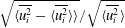 $\sqrt{\langle \overline{u_{i}^{2}}-\langle \overline{u_{i}^{2}}\rangle \rangle }/\sqrt{\langle \overline{u_{i}^{2}}\rangle }$, of 1.3 %, 1.9 % and 1.3 % in the
 $x_{1}$-,
 $x_{2}$- and
 $x_{3}$-directions, respectively, from the stereo PIV data, and 0.4 %, 0.7 % and 0.3 % from the scanning PIV data, implying that the flow is homogeneous relative to the mean flow. The velocity gradients also appear to be approximately locally homogeneous, with the largest spatial variation of the square of the gradients varying from
 $(\langle \overline{(\unicode[STIX]{x2202}u_{1}/\unicode[STIX]{x2202}x_{2})^{2}}-\langle \overline{(\unicode[STIX]{x2202}u_{1}/\unicode[STIX]{x2202}x_{2})^{2}}\rangle \rangle )/(\langle \overline{(\unicode[STIX]{x2202}u_{1}/\unicode[STIX]{x2202}x_{2})^{2}}\rangle )=7.4\,\%$ to
 $(\langle \overline{(\unicode[STIX]{x2202}u_{2}/\unicode[STIX]{x2202}x_{1})^{2}}-\langle \overline{(\unicode[STIX]{x2202}u_{2}/\unicode[STIX]{x2202}x_{1})^{2}}\rangle \rangle )/(\langle \overline{(\unicode[STIX]{x2202}u_{2}/\unicode[STIX]{x2202}x_{1})^{2}}\rangle )=13.6\,\%$ from the stereo PIV data, and from
 $(\langle \overline{(\unicode[STIX]{x2202}u_{3}/\unicode[STIX]{x2202}x_{1})^{2}}-\langle \overline{(\unicode[STIX]{x2202}u_{3}/\unicode[STIX]{x2202}x_{1})^{2}}\rangle \rangle )/(\langle \overline{(\unicode[STIX]{x2202}u_{3}/\unicode[STIX]{x2202}x_{1})^{2}}\rangle )=3.4\,\%$ to
 $(\langle \overline{(\unicode[STIX]{x2202}u_{3}/\unicode[STIX]{x2202}x_{3})^{2}}-\langle \overline{(\unicode[STIX]{x2202}u_{3}/\unicode[STIX]{x2202}x_{3})^{2}}\rangle \rangle )/(\langle \overline{(\unicode[STIX]{x2202}u_{3}/\unicode[STIX]{x2202}x_{3})^{2}}\rangle )=8.4\,\%$ from the scanning PIV data.
Table 5 shows an overview of the mean Reynolds stresses. In an isotropic flow, the diagonal values of the Reynolds stresses would be equal, and the remaining stresses would be zero, while in an axisymmetric flow, the tensor should follow the relation
 $$\begin{eqnarray}\overline{u_{i}u_{j}}=A\unicode[STIX]{x1D6FF}_{ij}+Bn_{i}n_{j},\end{eqnarray}$$
where  $\boldsymbol{n}$ is the unit vector for the symmetry axis and
 $\unicode[STIX]{x1D6FF}_{ij}$ is the Kronecker delta (Batchelor & Taylor Reference Batchelor and Taylor1946).
Reynolds stresses normalised by impeller frequency and radius,  $\langle \overline{u_{i}u_{j}}\rangle /((D/2)f)^{2}$.

The strong shear generated by the counter-rotating flow creates high turbulent fluctuations, and neither the mean flow nor the turbulent fluctuations in the tank are isotropic. There is, however, an axisymmetry along the  $x_{2}$-axis, with the constants in (B 1) equal to
 $A/((D/2)f)\approx 2.3$ and
 $B/((D/2)f)\approx 1.0$. Previous studies of von Kármán mixing flow have found that the ratio between fluctuations in the radial and axial directions is
 ${\sim}1.5$, while the off-diagonal terms are expected to be close to zero (Voth et al. Reference Voth, Satyanarayan and Bodenschatz1998). Therefore, the current measured ratios of 1.55 and 1.52 from the stereo and scanning PIV data agree well with previous results (Voth et al. Reference Voth, Porta, Crawford, Aelxander and Bodenschatz2002; Worth Reference Worth2010; Lawson Reference Lawson2015). Furthermore, the predicted Reynolds stresses from the two data sets are very similar, and vary by a maximum of
 $\overline{u_{i}u_{j}}/((D/2)f)^{2}=0.1$ for the square of the out-of-plane velocity, which corresponds to 4.3 % of
 $u_{rms}$.
The mean flow gradients are approximately constant across the measurement volume, and the values collected from the two data sets are presented in table 6. The results are similar, with a maximum deviation of  $\langle \unicode[STIX]{x2202}U_{i}/\unicode[STIX]{x2202}x_{i}\rangle /f=0.25$, again for the out-of-plane component. The result of constant gradients is an expected constant dissipation rate. The results from the scanning PIV data has small local variations:
 $\langle \overline{(\unicode[STIX]{x1D708}(\unicode[STIX]{x2202}u_{i}/\unicode[STIX]{x2202}x_{j})(\unicode[STIX]{x2202}u_{i}/\unicode[STIX]{x2202}x_{j})-\unicode[STIX]{x1D716})^{2}}\rangle /\langle \unicode[STIX]{x1D716}\rangle =0.8\,\%$. The dissipation rate is therefore assumed to have a constant value across the FOV.
Mean gradients in the flow normalised by impeller frequency calculated from the two data sets.

B.1.2 Comparison of flow topology between measurement methods
The flow topology is briefly characterised in terms of the distribution of enstrophy and dissipation, and then invariant quantities. Given that the full velocity gradient tensor is available from the volumetric measurements, the true dissipation rate can be directly calculated without assumptions using (B 2),
 $$\begin{eqnarray}\unicode[STIX]{x1D716}_{true}=2\unicode[STIX]{x1D708}\overline{\unicode[STIX]{x1D634}_{ij}\unicode[STIX]{x1D634}_{ij}},\end{eqnarray}$$
where the strain rate tensor,  $\unicode[STIX]{x1D634}_{ij}$, is evaluated from (B 3),
 $$\begin{eqnarray}\unicode[STIX]{x1D634}_{ij}=\frac{1}{2}\left(\frac{\unicode[STIX]{x2202}u_{i}}{\unicode[STIX]{x2202}x_{j}}+\frac{\unicode[STIX]{x2202}u_{j}}{\unicode[STIX]{x2202}x_{i}}\right).\end{eqnarray}$$
However, the same calculations cannot be made using the planar data, as the velocity gradient tensor is incomplete. Therefore, the dissipation rate is calculated using assumptions of axisymmetry, with the missing terms replaced according to George & Hussein (Reference George and Hussein1991) using (B 4).
 $$\begin{eqnarray}\displaystyle \unicode[STIX]{x1D716}_{axi} & = & \displaystyle 2\unicode[STIX]{x1D708}\left(\overline{\left(\frac{\unicode[STIX]{x2202}u_{1}}{\unicode[STIX]{x2202}x_{1}}\right)^{2}}+\overline{\left(\frac{\unicode[STIX]{x2202}u_{2}}{\unicode[STIX]{x2202}x_{2}}\right)^{2}}+\overline{\left(\frac{\unicode[STIX]{x2202}u_{3}}{\unicode[STIX]{x2202}x_{3}}\right)^{2}}+\overline{\left(\frac{\unicode[STIX]{x2202}u_{1}}{\unicode[STIX]{x2202}x_{2}}\right)^{2}}\right.\nonumber\\ \displaystyle & & \displaystyle +\left.\overline{\left(\frac{\unicode[STIX]{x2202}u_{2}}{\unicode[STIX]{x2202}x_{1}}\right)}^{2}+2\overline{\frac{\unicode[STIX]{x2202}u_{1}}{\unicode[STIX]{x2202}x_{2}}\frac{\unicode[STIX]{x2202}u_{2}}{\unicode[STIX]{x2202}x_{1}}}+\overline{\left(\frac{\unicode[STIX]{x2202}u_{3}}{\unicode[STIX]{x2202}x_{1}}\right)^{2}}+\overline{\frac{1}{2}\frac{\unicode[STIX]{x2202}u_{1}}{\unicode[STIX]{x2202}x_{1}}\frac{\unicode[STIX]{x2202}u_{3}}{\unicode[STIX]{x2202}x_{3}}}\right).\end{eqnarray}$$
The relation in (B 4) is usually used to estimate the mean dissipation rate, which also is the case for this work. In addition we use the instantaneous values of the two dissipation rates,  $\unicode[STIX]{x1D716}_{true}^{\prime }$ and
 $\unicode[STIX]{x1D716}_{axi}^{\prime }$ (where ′ implies that it is the instantaneous values which is considered) to compare the joint PDF and PDF of the two terms shown in figure 22, which, when compared to the distribution of the full dissipation,
 $\unicode[STIX]{x1D716}_{true}$, appears to be a good approximation. However, we would still like to emphasise that the instantaneous estimations of
 $\unicode[STIX]{x1D716}_{axi}^{\prime }$ are solely used to compare the two data sets. To assess the level of local axisymmetry, a test was performed by using the following relations derived in George & Hussein (Reference George and Hussein1991), where it is stated that
 $K_{1}=K_{2}$ in axisymmetric flow:
 $$\begin{eqnarray}\displaystyle & \displaystyle K_{1}=2\left.\left\langle \overline{\left(\frac{\unicode[STIX]{x2202}u_{2}}{\unicode[STIX]{x2202}x_{2}}\right)^{2}}\right\rangle \right/\left\langle \overline{\left(\frac{\unicode[STIX]{x2202}u_{1}}{\unicode[STIX]{x2202}x_{2}}\right)^{2}}\right\rangle , & \displaystyle\end{eqnarray}$$
 $$\begin{eqnarray}\displaystyle & \displaystyle K_{2}=2\left.\left\langle \overline{\left(\frac{\unicode[STIX]{x2202}u_{2}}{\unicode[STIX]{x2202}x_{2}}\right)^{2}}\right\rangle \right/\left\langle \overline{\left(\frac{\unicode[STIX]{x2202}u_{3}}{\unicode[STIX]{x2202}x_{2}}\right)^{2}}\right\rangle . & \displaystyle\end{eqnarray}$$
The values from the stereo PIV data were calculated to be 0.94 and 0.93 for  $K_{1}$ and
 $K_{2}$ respectively, giving a good indication that the flow is behaving locally axisymmetric.
(a) The p.d.f.s of dissipation rate  $\unicode[STIX]{x1D716}_{true}^{\prime }$, the dissipation rate based on axisymmetric assumptions
 $\unicode[STIX]{x1D716}_{axi}^{\prime }$, and the third component of the vorticity,
 $\unicode[STIX]{x1D714}_{3}^{2}$. Solid lines from scanning PIV data, and dashed lines from stereo PIV data. (b) Joint p.d.f. of dissipation rate
 $\unicode[STIX]{x1D716}_{true}^{\prime }$ and the enstrophy,
 $\unicode[STIX]{x1D714}^{2}$ from scanning PIV data. The contours are logarithmically spaced from
 $10^{-5}$ to
 $10^{-2}$.

To test the validity of these assumptions, and again compare the calculated velocity gradients of the two data sets, the PDF of  $\unicode[STIX]{x1D716}_{axi}^{\prime }$,
 $\unicode[STIX]{x1D716}_{true}^{\prime }$ and the third component of the vorticity vector squared,
 $\unicode[STIX]{x1D714}_{3}^{2}$ (where
 $\unicode[STIX]{x1D74E}=\unicode[STIX]{x1D735}\times \boldsymbol{u}$), based on the two data sets are compared in figure 22(a). There is an almost exact overlap of the PDFs of
 $\unicode[STIX]{x1D714}_{3}^{2}$ based on the two data sets, indicating that the gradients based on the two data sets have a very similar behaviour. As for the dissipation, the shape of the distributions of
 $\unicode[STIX]{x1D716}_{axi}^{\prime }$ and
 $\unicode[STIX]{x1D716}_{true}^{\prime }$ is similar, but the planar data tend to slightly overestimate extreme high and low dissipation events compared to the PDF of the full dissipation rate calculated from the volumetric data.
To evaluate the distribution of high gradient regions, the joint probability density function of enstrophy,  $\unicode[STIX]{x1D714}^{2}$, and dissipation rate is given in figure 22(b). The distribution shows good agreement with previous studies (Worth & Nickels Reference Worth and Nickels2011; Yeung, Donzis & Sreenivasan Reference Yeung, Donzis and Sreenivasan2012; Carter & Coletti Reference Carter and Coletti2018), demonstrating characteristic associated with high Reynolds number turbulent flows. The first quadrant, where high values of both
 $\unicode[STIX]{x1D716}$ and
 $\unicode[STIX]{x1D714}^{2}$ are present has an almost symmetric, pointed shape, indicating that extreme high values of the two terms occur simultaneously (Worth & Nickels Reference Worth and Nickels2011). The close agreement observed between the velocity gradient statistics using the two different measurement methods provides confidence that the more technically challenging volumetric measurements are consistent with the planar measurements, and that the volumetric data set is capable of capturing the important flow gradient characteristics.