




No CrossRef data available.
THE VALUE OF INFORMATION SHARING IN A TWO-STAGE SUPPLY CHAIN WITH PRODUCTION CAPACITY CONSTRAINTS: THE INFINITE HORIZON CASE
Published online by Cambridge University Press: 16 April 2004
Abstract
We study the value of information sharing in a two-stage supply chain with a single manufacturer and a single retailer in an infinite time horizon, where the manufacturer has finite production capacity and the retailer faces independent demand. The manufacturer receives demand information even during periods of time in which the retailer does not order. Allowing for time-varying cost functions, our objective is to characterize the impact of information sharing on the manufacturer's cost and service level. We develop a new approach to characterize the induced Markov chains under cyclic order-up-to policy and provide a simple proof for the optimality of cyclic order-up-to policy for the manufacturer under the average cost criterion. Using extensive computational analysis, we quantify the impact of information sharing on the manufacturer's performance in an infinite time horizon under both i.i.d. demand and independent but nonstationary demand.
Information
- Type
- Research Article
- Information
- Probability in the Engineering and Informational Sciences , Volume 18 , Issue 2 , April 2004 , pp. 247 - 274
- Copyright
- © 2004 Cambridge University Press
1. INTRODUCTION
Information technology is an important enabler of efficient supply chain strategies. Indeed, much of the current interest in supply chain management is motivated by the possibilities introduced by the abundance of data and the savings inherent in sophisticated analysis of these data. For example, information technology has changed the way companies collaborate with suppliers and customers. These collaborations, which allow companies to share sensitive demand information with their suppliers in real time, have achieved huge success in practice in terms of inventory reduction, service level improvement, and quick response to market changes (Stein and Sweat [31]).
The benefits of sharing demand-related information among supply chain partners has been explored by many authors: for example, the Bullwhip effects reduction (Lee, Padmanabhan, and Whang [21] and Chen, Drezner, Ryan, and Simchi-Levi [5]) and the inventory cost reduction (Hariharan and Zipkin [13], Gallego and Ozer [10], Gavirneni, Kapuscinski, and Tayur [11], Aviv and Federgruen [2], Cachon and Fisher [3], Chen [4], and Simchi-Levi and Zhao [28]). These studies cover a broad range of production–distribution systems, such as single-supplier and single-retailer systems (Gavirneni et al. [11], Simchi-Levi and Zhao [28]), single-supplier, multiretailer systems (Aviv and Federgruen [2], Cachon and Fisher [3]), and multistage series systems (Chen [4] and Chen et al. [5]). An excellent review of recent research can be found in Cachon and Fisher [3].
In this article, we focus on a single capacitated manufacturer serving a single retailer. The retailer faces independent demand and the objective is to analyze the impact of information sharing on the manufacturer's cost and service levels. The impact of information sharing on a capacitated manufacturer has been analyzed by several authors. Aviv and Federgruen [2] analyzed a single-supplier, multi-retailer system in which retailers faced random demand and shared inventories and sales data with the supplier. They analyzed the effectiveness of a Vendor Managed Inventory (VMI) program where sales and inventory data are used by the supplier to determine the timing and the amount of shipments to the retailers. For this purpose, they compared the performance of the VMI program with that of a traditional, decentralized system, as well as a supply chain in which information is shared continuously, but decisions are made individually (i.e., by the different parties). Their focus in the three systems analyzed was on minimizing long-run average cost. Aviv and Federgruen reported that information sharing reduces systemwide cost by 0–5%, whereas VMI reduces cost, relative to information sharing, by 0.4–9.5% and on average by 4.7%. They also showed that information sharing could be very beneficial for the supplier.
The work by Gavirneni et al. [11] analyzed a two-stage supply chain with a single capacitated supplier and a single retailer. In this periodic review model, the retailer made ordering decisions every period, using an (s,S) inventory policy, and transferred demand information every time an order decision was made, independent of whether an order was made. Assuming zero transportation lead time, they showed that the benefit (i.e., the supplier cost savings due to information sharing) increased with production capacity and it ranged from 1% to 35%.
The focus of this article is on the benefits of information sharing for a capacitated supplier in a two-stage supply chain with an infinite time horizon. In this model, the retailer shares demand information with the supplier even at times during which she does not make order decisions. This is clearly the case in many industries in which demand information can be shared very frequently (e.g., every second or every minute) while orders are placed less frequently (e.g., every day or every week). A recent article by Simchi-Levi and Zhao [28] studied this model in a finite time horizon setting. They show that by sharing demand information, the supplier can reduce its inventory cost substantially while maintaining the same service level to the retailer.
The optimal control of a periodic review production–inventory system in an infinite time horizon is a classical Markov decision problem with infinite state space and unbounded cost function. The literature on these problems is quite voluminous (see, e.g., Heyman and Sobel [15] and Puterman [24] for a general theory of the Markov decision process; Karlin [17], Zipkin [32], Sethi and Cheng [27], and Song and Zipkin [30] for systems with time-varying parameters; Federgruen and Zipkin [7,8] for systems with production capacity constraints). Finally, Aviv and Federgruen [1] and Kapuscinski and Tayur [16] have analyzed periodic review production–inventory systems with capacity constraints and time-varying parameters and their results are most relevant to our model. They show that a modified cyclic order-up-to policy (i.e., a modified order-up-to policy with periodically varying order-up-to levels) is optimal under both discounted and average cost criterion. This is done by verifying the optimality conditions developed by Sennott [26] and Federgruen, Schweitzer, and Tijms [6].
In the next section, we describe our model and identify the differences between our model and results and those of Aviv and Federgruen [1] and Kapuscinski and Tayur [16].
2. THE MODEL
Consider a single product, periodic review, two-stage production–inventory system with a single capacitated manufacturer and a single retailer facing independent demand and using an order-up-to inventory policy. In practice, many retailers place orders periodically (e.g., every week or every month). Thus, we assume that the retailer places an order every T time periods (e.g., 7 days) to raise his inventory position to a target level. The manufacturer receives demand information from the retailer every τ units of time (τ ≤ T). For instance, the retailer places an order every week but provides demand information every day. We refer to the time between successive orders as the ordering period and the time between successive information sharing as the information period. Of course, in most supply chains, information can be shared almost continuously (e.g., every second) while decisions are made less frequently (e.g., every day). Thus, information periods really refers to the time interval between successive uses of the information provided.
The sequence of events in our model is as follows. At the beginning of an ordering period, the retailer reviews her inventory and places an order to raise the inventory position to the target inventory level. The manufacturer receives the order from the retailer, fills the order as much as she can from stock, and then makes a production decision. If the manufacturer cannot satisfy all of a retailer's order from stock, then the missing amount is backlogged. The backorder will not be delivered to the retailer until at least the beginning of the next ordering period. Finally, transportation lead time between the manufacturer and the retailer is assumed to be zero. Similarly, at the beginning of an information period, the retailer transfers POS (Point of Sales) data of previous information period to the manufacturer. Upon receiving this demand information, the manufacturer reduces this demand from her inventory position although she still holds the stock, and then she makes a production decision.
To simplify the analysis, we assume that demand is stationary across the ordering periods, whereas the demand distribution may vary across different information periods within one ordering period. For example, grocery retailers typically face much higher demand during weekends than week days. At the same time, these retailers are replenished once a week. Since grocery retailers cannot anticipate future shortages from the manufacturer, they are not able to inflate order-up-to levels to protect themselves from future shortages. Hence, we assume in our model that the retailer's target order-up-to level is constant for all the ordering periods; that is, every ordering period, the retailer raises her inventory position (outstanding order plus on-hand inventory minus backorders) to a constant level. Any unsatisfied demand at the retailer is backlogged; thus, the retailer transfers external demand of each ordering period to the manufacturer. The manufacturer has a production capacity limit (i.e., a limit on the amount the manufacturer can produce per unit of time) and the manufacturer runs her production line always at this capacity limit.
Let N = T/τ be an integer which represents the number of information periods in one ordering period. We index information periods within one ordering period 1,2,…,N, where 1 is the first information period in the ordering period and N is the last. Let C denote production capacity in one information period τ, c is the production cost per item, and 0 < β < 1 is the time discounted factor for each information period.
Since we calculate inventory holding cost for each information period, we let h be the inventory holding cost per unit product per information period. Evidently, one unit of product kept in inventory for n information periods, n = N,N − 1,…,1, will incur a total inventory cost hn = h(1 + β +···+ βn−1).
Due to the finite production capacity, the manufacturer produces to stock. For every item backlogged at the end of each ordering period, the manufacturer pays π as a penalty cost. It is easy to see that the earlier the manufacturer produces during a single ordering period, the longer she will carry this inventory, thus the higher the inventory holding cost. On the other hand, postponing production too long may result in heavy penalty cost due to the finite production capacity.
We use Di to denote the end-user demand in the information period i, i = 1,…,N. Di is assumed to be independent, its distribution only depends on i, and its mean is defined as EDi. To simplify the analysis, we assume that costs do not change from information period to information period; later, we will demonstrate that our results can be easily extended to include cases where costs change periodically within one ordering period but are the same across different ordering periods.
We start by considering a finite time horizon model with M ordering periods. Index the ordering periods from 0 to M − 1, where the 0 ordering period is the first one and the M − 1 ordering period is the last one. The finite horizon starts in the first ordering period at the beginning of the jth information period, 1 ≤ j ≤ N. Consider the ith information period, i = 1,2,…,N, in ordering period m, m = 0,1,…,M − 1. Of course, mN + i ≥ j. We refer to this information period as the mN + i information period. For instance, information period mN + 1 is the first information period in the mth ordering cycle. We refer to this indexing convention as a forward indexing process.
Define x to be the inventory position at the beginning of the ith information period, and Si to be the state space for x. Let y − x be the amount produced in that information period, y ∈ Ax, and Ax be the set of feasible actions. Let ξ(x,y,D) be the transition function and D be the demand. In our case, Ax = [x,x + C] and ξ(x,y,D) = y − D.
It is easy to verify that gmN+i(x,y), i = 1,2,…,N, m = 0,…,M − 1, the expected inventory and production cost in information period mN + i, given that the period starts with an inventory position x, and y − x items are produced in that period, can be written as

where E(·) is the expectation with respect to DN and

Because the items produced in the ith information period are carried over until the end of the ordering period, an inventory holding cost equal to hN−i(y − x) is charged in this information period.
Since gmN+i(x,y) depends only on i and not m, we can write gmN+i(x,y) = ri(x,y), ∀m = 0,1,…,M − 1 and ∀i = 0,1,…,N. Furthermore, ri(x,y) can be written as the sum of a function of x (φi(x)) and a function of y(φi(y)), where


Finally, we assume the salvage cost function gMN+1 = 0.
We define the optimal policy under the discounted cost criterion as follows. Let σ = {σ1,σ2,…} be any feasible policy where σk is a function depending on the initial inventory position in period k (i.e., σk = σk(x) and σk(x) ∈ Ax for all k). Let Π be the set of all feasible policies. Define the expected discounted cost from the ith information period in the first ordering period until the end of the horizon when M → ∞, as

where E(·) denotes the expectation with respect to demand in all information periods and xi is the initial inventory position of the ith information period for i = 1,2,…,N. A policy σ* = {σ1*,σ2*,…} ∈ Π is called optimal under the discounted cost criterion if for all x ∈ S and i,

Similarly, the optimal policy in an infinite time horizon under the average cost criterion can be defined. Following Heyman and Sobel [14], the performance measure for any feasible policy δ = {δ1,δ2,…} ∈ Π under the average cost criterion is defined as

A policy δ* is optimal if it minimizes Gi(x,δ) for all x and i over Π.
It is easily seen that in the information sharing model, except for those periods in which orders are placed, the cost function φi(y) tends to negative infinity as y → −∞ (y → −∞ implies that the manufacturer allows for infinite backorders). This is true because although demand is observed by the manufacturer in every information period, it only needs to be satisfied at the end of every ordering period. Thus, the penalty cost is charged only at the end of ordering periods, whereas the inventory holding cost is charged in every information period. Clearly, this issue was not addressed in the models analyzed by Aviv and Federgruen, and Kapuscinski and Tayur since they assumed φi(y), for all i, were bounded from below.
To further explain the difference between this model and previous models, let us consider the following three cases. First, if the manufacturer only has inventory holding cost but no penalty cost for all periods, then the optimal policy is not finite; that is, the optimal policy does not have a finite order-up-to level because producing nothing in all periods is clearly the optimal policy. Second, if the manufacturer has both inventory holding cost and penalty cost for all periods, then we have the models studied by Aviv and Federgruen [1] and Kapuscinski and Tayur [16]. Finally, if in some periods the manufacturer only has inventory holding cost, whereas in other periods she has both holding and penalty cost, then it is not clear whether there exists an optimal policy with a finite order-up-to level.
Thus, the objective of this article is twofold: First, characterize the optimal policy for the information sharing model under both discounted and average cost criteria; second, quantify the benefits and identify the conditions under which information sharing is most beneficial for the manufacturer in an infinite time horizon; that is, characterize how frequently information should be shared and when it should be shared so that the manufacturer can maximize the potential benefits.
We show that a cyclic order-up-to policy is optimal under both discounted and average cost criteria. Although the optimal policy has the same structure as those of Aviv and Federgruen [1] and Kapuscinski and Tayur [16], our analysis of the average cost criterion, which is based on the vanishing discount method (Heyman and Sobel [14]), is quite different from theirs.
One of the major difficulties in proving the average cost criterion is to characterize the Markov chain induced by the optimal policy under the discounted cost criterion. To address this issue, we introduce a new method to construct and relate Markov chains in a common state space. Together with the Foster's criterion and the Lyapunov function, this method allows us to show that each of the Markov chains induced by any finite cyclic order-up-to policy has a single irreducible positive recurrent class and finite long-run average cost under certain nonrestrictive conditions (Section 3). Then, in Section 4, we provide a simple proof for the cyclic order-up-to policy to be optimal under the average cost criterion. Finally, extensive computational study is conducted in Section 5, using IPA (Infinitesimal Perturbation Analysis), to quantify the impacts of frequency and timing of information sharing, with a particular focus on the differences between finite and infinite time horizons, and nonstationary external demand.
3. PROPERTIES OF CYCLIC ORDER-UP-TO POLICY
In this section, we study the Markov processes associated with any cyclic order-up-to policy and identify conditions under which they are positive recurrent and have finite steady state average cost. The conditions are similar to those identified by Aviv and Federgruen, and Kapuscinski and Tayur, but the analysis is quite different.
At this point, it is appropriate to remind the reader of the definition of a cyclic order-up-to policy in a capacitated production system. In such a system, every time period the manufacturer produces up to the target inventory position if there is enough production capacity, otherwise the manufacturer produces as much as the production capacity allows. Of course, the target inventory position may vary periodically.
Consider the information sharing model with the cost function ri(x,y) ∼ O(|x|ρ) + O(|y|ρ), where ρ is a positive integer. Define a cyclic order-up-to policy as a policy with different order-up-to levels for different information periods, but these levels are the same for the same information period in different ordering periods; that is, the order-up-to level in information period mN + i is the same for all m but may be different for different i, i = 1,2,…,N.
Let Di, i = 1,…,N, be the random variable representing demand in information period mN + i for all m; demand is assumed to take discrete values. Consider a cyclic order-up-to policy with levels a1,a2,…,aN, and define the shortfall processes {smN+i,m = 0,1,…} for different i = 1,…,N as smN+i = ai − ymN+i if we are in period mN + i and ymN+i is the inventory position at the end of this period before demand is realized. Clearly, the shortfall may be negative. When it is positive, it represents the difference between what the manufacturer likes to produce and what the production capacity allows the manufacturer to produce. When the target inventory level, ai, is lower than the initial inventory position at the beginning of the period, the shortfall is negative. The dynamics of the shortfall is

If excessive stock is returned when the inventory position is higher than the order-up-to level, then the dynamics of shortfall processes {smN+ir,m = 0,1,…} for i = 1,…,N is smN+i+1r = (ai+1 − ai + smN+ir + Di − C)+. We refer to this policy as an order-up-to policy with returns.
Proving that the shortfall process induced by a constant order-up-to policy has a finite steady state average cost is known to be difficult (see, e.g., the appendix of Kapuscinski and Tayur [15]). Proving that each of the shortfall processes induced by a general cyclic order-up-to policy has finite steady state average cost and a single irreducible positive recurrent class is even more difficult because of the more complicated transition matrices.
The following methods have been applied in the literature to address these issues. Aviv and Federgruen showed that if (1) E(Dil) < ∞ for all positive integers l ≤ ρ + 1 and i = 1,…,N and (2)

, then for any finite order-up-to policy, the shortfall process has a finite set of states such that it can be reached with finite expected cost from any starting state. Kapuscinski and Tayur's method has the following two steps: They first characterized the shortfall process under the order-up-to zero policy. Then, they related a cyclic order-up-to policy to an order-up-to zero policy and proved that in steady state, E(|xi|ρ) and E(|si|ρ) are finite for a cyclic order-up-to policy under similar conditions as those proved by Aviv and Federgruen, namely (1) E(Di2ρ+2) < ∞ for i = 1,…,N and (2)

.
In this section, we introduce a new approach to prove that {xmN+i,m = 0,1,…}, the inventory positions at the beginning of mN + ith information period, {ymN+i,m = 0,1,…}, the inventory position at the end of period mN + i but before demand is realized, and {smN+i,m = 0,1,…}, the shortfall in period mN + i, induced by any finite cyclic order-up-to policy give rise to Markov chains with a single irreducible and positive recurrent class and finite steady state average cost under the same condition as Aviv and Federgruen; that is, we require (1) E(Dil) < ∞ for all positive integers l ≤ ρ + 1 and i = 1,…,N and (2)

.
This is done as follows. First, using the Foster's criterion and the Lyapunov function, we show that the Markov chain induced by an order-up-to constant policy has the following properties: (i) single irreducible and positive recurrent class and (ii) finite steady state average cost. The same properties hold true for the Markov chain induced by a cyclic order-up-to policy with returns. Then, we relate Markov chains induced by a cyclic order-up-to policy and a cyclic order-up-to policy with returns in a common state space. This allows us to prove, under mild conditions, that properties such as positive recurrence and finite steady state average cost hold true for systems using a cyclic order-up-to policy if and only if they hold true for systems using a similar policy with returns.
We begin our analysis by presenting new proofs for the positive recurrence and finite steady state average cost of the order-up-to zero policy. To simplify the analysis, let us assume Pr(Di < 0) = 0,∀i.
Proposition 3.1: Given order-up-to zero policy, the inventory positions {xmN+i,m = 0,1,…} and {ymN+i,m = 0,1,…} and the shortfall process {smN+i,m = 0,1,…} for i = 1,…,N generate discrete-time Markov chains (DTMC) with single irreducible and positive recurrent class if

.
Proof: See the appendix for details. █
The proof that the steady state average cost associated with an order-up-to zero policy is finite is based on the following lemma.
Lemma 3.2: Consider an irreducible and aperiodic Markov chain {Xn,n = 0,1,…} with a single period cost function r(·). r(·) is continuous and bounded from below. Assume that there exists a Lyapunov function V(·) mapping the state space S to [0,∞) and a constant η such that

Then, given an initial state x0 with V(x0) < ∞, the Markov chain Xn has finite steady state average cost if Xn is positive recurrent.
This lemma is a variation of the Foster's second criterion by Meyn and Tweedie [23; see Theorem 14.0.1 (f-regularity)]; thus, we omit the proof and refer to Simchi-Levi and Zhao [29] for technical details. The lemma implies the following.
Lemma 3.3: Consider the order-up-to zero policy. If E((Di)k) < ∞ for all integers

, then in steady state, the following hold:

Proof: See the appendix for details. █
Proposition 3.1 and Lemma 3.3 can be extended to any finite cyclic order-up-to policy with returns as follows.
Proposition 3.4: Consider any finite cyclic order-up-to policy with returns. If

for any positive integer k ≤ ρ + 1 and ∀i, then the following hold:

Proof: Assume ai,i = 1,…,N, to be the order-up-to levels. We only need to transform this policy to an order-up-to zero policy and then apply Proposition 3.1 and Lemma 3.3.
Consider ymN+ir, the inventory positions at the end of period mN + i before demand is realized. For simplicity, we drop the subscript mN. The system dynamics is yi+1r = min{yir − Di + C,ai+1} = ai+1 + (yir − ai+1 − Di + C)−, where x− = min{0,x}. Let zi′ = yir − ai and Di′ = Di + (ai+1 − ai); then,

. For zi′ and Di′, this is order-up-to zero policy, where demand Di′ can be negative but bounded from below.
Notice that the shortfall processes associated with this order-up-to zero policy have state space {0,1,2,…} even if demand can be negative (due to return). Using proofs similar to those of Proposition 3.1 and Lemma 3.3, we can show that the same results hold for this order-up-to zero policy if there exists a positive constant di so that Pr{Di < −di} = 0, ∀i = 1,2,…,N. █
We now introduce a method to construct and relate Markov chains induced by a cyclic order-up-to policy and a cyclic order-up-to policy with returns in a common state space. Consider two inventory systems: One uses a cyclic order-up-to policy and the other uses a corresponding policy with returns. The key idea of the method is to characterize the gap between the inventory position processes without returns, ymN+i, and with returns, ymN+ir, assuming that both inventory systems start with the same initial inventory level and face the same stream of demand.
Lemma 3.5: Consider two inventory systems with cyclic order-up-to levels a1,…,aN, for N ≥ 2: one system without returns and the second one with returns. If the two systems start with the same initial state x0 ≤ max{a1,…,an} and face the same stream of random demand, then the stochastic processes {zmN+i = ymN+i − ymN+ir,m = 0,1,…} have the following properties for all i:
(i) zmN+i ≥ 0 for all m.
(ii) zmN+i ≤ max{a1,…,aN} − min{a1,…,aN} for all m.
Proof: The proof is by induction. Clearly, z1 = 0. Consider period mN + i and assume 0 ≤ zmN+i ≤ max{a1,…,aN} − min{a1,…,aN}. We distinguish between the following two cases. In the first case, ai ≤ ai+1 and in the second case, ai > ai+1.
ai ≤ ai+1: There are two subcases to consider. (1) xmN+i+1 and xmN+i+1r are no larger than ai+1. In this case, ymN+i+1 = min{xmN+i+1 + c,ai+1} and ymN+i+1r = min{xmN+i+1r + c,ai+1} and, hence,

(2) xmN+i+1 > ai+1 ≥ xmN+i+1r. This can only occur if N > 2 and ai+1 < max{a1,…,aN}. Clearly, ymN+i+1 = xmN+i+1 and ymN+i+1r = min{xmN+i+1r + c,ai+1}, which implies that

ai > ai+1: In this case there are three possible subcases: (1) xmN+i+1 and xmN+i+1r are no larger than ai+1; (2) xmN+i+1 > ai+1 ≥ xmN+i+1r; (3) xmN+i+1 and xmN+i+1r are larger than ai+1. The proof of the first two subcases is identical to the proof in the previous case. Consider subcase 3 and observe that in this case ymN+i+1 = xmN+i+1 and ymN+i+1r = ai+1 and, hence,

█
Remark: If x0 > max{a1,…,aN}, then the state space for {zmN+i,m = 0,1,…} is {0,1,…,x0 − min{a1,…,aN}}, ∀i.
Theorem 3.6: Consider two arbitrary irreducible DTMCs {xn,n = 0,1,…} and {yn,n = 0,1,…} starting with the same initial state. If their difference process {zn = xn − yn,n = 0,1,…} has finite state space Sz, then xn is positive recurrent if and only if yn is positive recurrent. Also, xn has certain finite steady state moments if and only if the same steady state moments of yn are finite.
Proof: First, we show that xn is positive recurrence if yn is positive recurrent. Define Sx and Sy to be the state space for {xn,n = 0,1,…} and {yn,n = 0,1,…}, respectively. Assume that yn is positive recurrent; using contradiction, we assume xn is transient or nonrecurrent for all of its state. Since yn = xn − zn and y0 = x0, we have

Since Sz has only a finite number of states and xn is transient or nonrecurrent, Pr{yn = i|y0} → 0 as n → ∞ for i ∈ Sy. This contradicts the assumption that yn is positive recurrent (see Kulkarni [20, p. 80, Theorem 3.4], and Kemeny, Snell, and Knapp [19, p. 36, Prop. 1-61]).
Second, assume that yn has finite steady state moments E(|y|l) for 0 < l ≤ ρ, where ρ is a positive integer. Consider

Taking the limit n → ∞ on both sides, we obtain

where c1,…,cρ are positive finite constants and |Sz| is the size of the state space for zn.
The necessary condition can be easily proved in a similar way. █
Lemma 3.5 and Theorem 3.6 provide a method to simplify Markov chains with infinite state space and complicated dynamics. Finally, we have the following corollary.
Corollary 3.7: Consider any finite cyclic order-up-to policy σ. If

for all i and positive integers k such that k ≤ ρ + 1, then the following hold:

converges to a finite value independent of initial period i and initial state x.
Proof: Parts (i)–(iv) are the direct results of Theorem 3.6, Lemma 3.5, and Proposition 3.4; thus they do not need a proof.
To prove part (v), notice that

in steady state is due to the assumption that ri(x,y) ∼ O(|x|ρ) + O(|y|ρ). Since the shortfall processes and thus ymN+i and xmN+i+1 give rise to Markov chains with single irreducible and positive recurrent class, we let the steady state distribution for (x,y) in the ith information period be p(x,y)i, where (x,y) ∈ Ωi (the feasible region of (x,y)), then

must converge since the summation is over at most a countable number of positive values and it is bounded from above. Finally, applying Proposition 1-61 (arithmetic average) of Kemeny et al. [19], the long-run average cost converges and equals the steady state average cost. █
4. A MARKOV DECISION PROCESS
Our objective in this section is to discuss the discounted and average cost criterion and present finite optimal policies for the information sharing model. For the discounted cost criterion, we follow Aviv and Federgruen [1] and specify conditions under which the cyclic order-up-to policy is optimal and the optimal order-up-to levels are finite. Other methods can be found in Heyman and Sobel [14], Federgruen and Zipkin [8], and Kapuscinski and Tayur [16].
For the average cost criterion, Sennott [25] and Federgruen et al. [6] introduced conditions under which there exists an optimal policy for general Markov decision processes (MDPs). Thus, one way to characterize the optimal policy is to verify that these conditions hold in our case. In fact, Aviv and Federgruen [1] and Kapuscinski and Tayur [16] have applied this method in their analysis.
We apply a different approach based on the vanishing discount method. For this purpose, we observe that in our model, the optimal policy under the discounted cost criterion can be characterized by a finite set of critical numbers (i.e., order-up-to levels). Thus, to prove the existence of an optimal policy under the average cost criterion, we only need to specify conditions (see Theorem 4.3) for the optimal order-up-to levels under the discounted cost criterion, instead of conditions on the entire policy.
To specify these conditions, we apply a result from Aviv and Federgruen [1]; namely that under certain conditions, the optimal order-up-to levels in the discounted cost criterion are uniformly bounded for all 0 < ε ≤ β < 1. We extend this result to the information sharing model (see Proposition 4.2), in which φi(y) is unbounded from both above and below for some i. This result, together with the results that long-run average cost is finite (Corollary 3.7), implies that a cyclic order-up-to policy is optimal under the average cost criterion (Theorem 4.3). We start by presenting conditions under which the optimal policy in the discounted cost case is a finite cyclic order-up-to policy.
Following convention, we index periods in a reverse order starting at the end of the planning horizon. Let m = 0 be the last ordering period and m = M − 1 be the first ordering period. We set i = N for the first information period and i =1 for the last information period in any ordering period. Thus, period mN + i represents the ith information period in the (m − 1)st ordering period. Finally, let gmN+i(x,y) = ri(x,y) denote the single period expected cost in this information period. We refer to this indexing as backward index and we will only use backward index in this section.
Let UmN+iβ(x) be the minimum expected total costs if there are mN + i periods remaining in the planning horizon, starting with an initial state x. Let the salvage cost U0β ≡ 0, and, hence,

where E(·) is the expectation with respect to Di. Observe that ri(x,y) can be written as the sum of a function of x (φi(x)) and a function of y (φi(y)), where


Thus, the following recursion must hold:

Observe that in the very first information period (i.e., information period (M − 1)N + N = MN) of the entire planning horizon, we have to add hN x+ to UMNβ(x) to account for the holding cost of initial inventory.
The dynamic programming model has the following properties:
1. The cost function ri(x,y) for each information period i = 1,…,N is positive and convex in y. Thus, the following property, proved in Kapuscinski and Tayur [16], holds: UmN+iβ(x) ≥ U(m−1)N+iβ(x) for any x, m = 1,…,M and i = 1,…,N.
2. ri(x,y) = φi(x) + φi(y) for all i, and there exists a positive integer ρ so that φi(x) ∼ O|x|ρ and φi(y) ∼ O|y|ρ. From Proposition 3.7, the total expected discounted cost using cyclic order-up-to policy is finite if

for any positive integer l ≤ ρ + 1, ∀i. This implies that UmN+iβ(x) converges pointwise to a finite value for any finite x and for all i (Heyman and Sobel [14, Thm.8-13]). Let Uiβ(x) denote the convergence point of UmN+iβ(x).
3. JmN+iβ(y) is convex in y, for all m and i. Furthermore, lim|y|→+∞ JmN+i(y) → +∞ for all m and i if βN−1π > c + hN−1. The main difficulty in proving that a cyclic order-up-to policy with finite target levels is optimal for this model is that the function φi(y) may be unbounded from both above and below. To overcome this difficulty, we need to aggregate N consecutive information periods and identify conditions under which the cost function for all these periods tends to positive infinity as the action variables approach either positive or negative infinity. Following the analysis of Simchi-Levi and Zhao [31], a sufficient condition is βN−1π > c + hN−1. Intuitively, this condition implies that the discounted penalty cost has to be larger than the sum of the production cost and inventory holding cost for a single ordering period so that the manufacturer should produce even in the first information period given that the initial inventory position is sufficiently low.
Theorem 4.1: For the Markov decision process defined in Eq. (19), if

then the following hold:
(1) Order-up-to policy is optimal for any m and i.
(2) Optimal order-up-to levels ymN+i* are bounded as m → +∞.
(3) JmN+i(y) converges to Ji(y) for all y,i, and every limit of ymN+i* is a minimal point for Ji(x).
(4) Cyclic order-up-to policy is optimal under the discounted cost criterion.
Proof: Since JmN+iβ(y) is a convex function of y and lim|y|→+∞ JmN+iβ(y) → +∞ for all m and i, the order-up-to policy is optimal for all m and i. Since UmN+iβ(x) is bounded from above for any m and finite x, order-up-to levels are finite as m → +∞ because of (b) (see the proof of Theorem 2 in Aviv and Federgruen [1]). Notice that UmN+iβ(x) is nondecreasing and converges to Uiβ(x), which implies JmN+iβ(y) is nondecreasing and converges to, say, Jiβ(y), due to the monotone convergence theorem. Hence, part 3 is true (also see the proof of Theorem 2 in Aviv and Federgruen [1]). Finally, parts 1–3 imply that cyclic order-up-to policy is optimal under the discounted cost criterion. █
We now extend Theorem 3(b) of Aviv and Federgruen [1] to our model.
Proposition 4.2: For the Markov decision process defined by Eq. (1), if the conditions of Theorem 4.1 are satisfied, then the optimal order-up-to levels yi*,i = 1,2,…,N, under the discounted cost criterion are uniformly bounded both from above and from below for any 0 < ε ≤ β < 1.
Since the extension follows a similar proof technique to the one in Aviv and Federgruen, we omit the proof and refer to Simchi-Levi and Zhao [29] for technical details. We are ready to characterize the average cost criterion.
Theorem 4.3: Consider the information sharing model and assume the following:
(a) Cyclic order-up-to policy is optimal under the discounted cost criterion.
(b) For all 0 < ε ≤ β < 1, the optimal order-up-to levels under the discounted cost criterion are uniformly bounded both from above and from below.
(c) The long-run average cost of any finite cyclic order-up-to policy converges to a finite value.
If these conditions are satisfied, then a cyclic order-up-to policy is optimal under the average cost criterion.
Proof: Consider a sequence of β1,β2,…,βj,…↑1 as j → ∞. Since the optimal order-up-to levels under the discounted cost criterion are uniformly bounded from both above and below for all 0 < ε ≤ β < 1, there must exist a finite cyclic order-up-to policy f and a subsequence jn → ∞ so that f is the optimal policy for all Uiβjn(x), ∀i = 1,2,…,N.
Since we can show that for any finite cyclic order-up-to policy σ,

converges to a finite value which is independent of the initial period i and initial state x (see Corollary 3.7); then, by Tauberian theory (Heyman and Sobel [14, p.172]),

The last inequality is justified by the Lemma A2 of Sennott [25]. █
Finally, we combine Theorem 4.3, 4.1, Corollary 3.7 and Proposition 4.2, to get
Corollary 4.4: In the information sharing model, if

then cyclic order-up-to policy is optimal under the average cost criterion.
5. COMPUTATIONAL RESULTS
In this section, we report on an extensive computational study conducted to develop insights about the benefits of information sharing. Our goal is to determine situations in which information sharing provides significant cost savings relative to supply chains with no information sharing in the infinite time horizon. For this purpose, we first examine the impact of the production capacity and the frequency and timing of information sharing on cost savings. This is followed by a systematic comparison between finite and infinite time horizons for i.i.d. external demand. Then, we study the impact of independent but nonstationary demand on the benefits of information sharing. In the computational study, we focus on the average cost criterion and compute the optimal order-up-to levels and cost by employing IPA (Fu [9] and Glasserman and Tayur [12]).
In the model with no information sharing, we assume that the retailer only places orders to the manufacturer at the end of each ordering period. Since the demand is backlogged and the retailer uses an order-up-to policy with constant order-up-to level, the order placed by the retailer is equal to the total demand in one ordering period. Furthermore, we assume that the manufacturer knows the retailer's ordering policy and, therefore, the demand distribution of one ordering period. Finally, we assume that the manufacturer has the same production capacity per information period and charges the same inventory holding cost per item per information period in the no-information-sharing model as in the information sharing model.
The model with no information sharing can be considered as a special case of the information sharing model. Indeed, consider an instance of the model with no information and construct an information sharing model in which demand in every information period within an ordering period is exactly zero except in the last information period. Demand in this information period equals the total demand during that ordering period. This information sharing model has the same dynamic programming formulation as the model with no information sharing. Thus, the dynamic program designed to solve the information sharing model can be applied to solve the model in which information is not shared. Finally, a finite cyclic order-up-to policy is optimal for the model with no information sharing under both the discounted and the average cost criterion.
In all of the numerical studies, we set the production cost c = 0 and focus on holding and penalty costs. The initial inventory position, x, at the beginning of the first ordering period is set to be zero without loss of generality.
5.1. i.i.d. Demand
In this subsection, external demand is assumed to be i.i.d. To identify situations in which the manufacturer can achieve significant benefits from information sharing and to compare the cost savings between finite and infinite time horizons, we examine the cases with variation of the following parameters: production capacity, the number of information periods in one ordering period, and the time when information is shared.
5.1.1. The effect of production capacity.
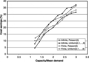
To explore the impact of production capacity on the benefit of information sharing in an infinite time horizon, we illustrate in Figure 1 the percentage cost savings from information sharing relative to no information sharing as a function of the production capacity. To compare with the finite time horizon, we also show in Figure 1 the percentage cost savings from information sharing when the planning horizon includes only one ordering period (Simchi-Levi and Zhao [28]).

The impact of the production capacity, i.i.d. demand.
The demand distribution of one information period are Poisson(5) and Uniform(0,1,…,9), and there are four information periods in each ordering period. The inventory holding cost per ordering period is set to be a constant $4 per unit product for all cases. Thus, the inventory holding cost per information period is $1 per unit. For each demand distribution and each capacity level, we consider the cases where the ratio of penalty cost to holding costs in one ordering period is $4.75.
The computational study reveals that, as production capacity increases, the cost saving percentage increases in both finite and infinite time horizons. Indeed, it increases from about 5% to about 35% as capacity over mean demand varies from 1.2 to 3. This is quite intuitive, since as production capacity increases, the optimal policy would postpone production as much as possible and take advantage of all information available prior to the time production starts. Similarly, if the production capacity is limited, then information is not very beneficial because the production quantity is mainly determined by capacity, not realized demand.
We would like to point out that this result is valid only when production capacity is finite. Indeed, if production capacity is large enough (e.g., infinite), then the manufacturer's optimal production policy is obviously to produce to order. Thus, in this case the manufacturer does not benefit from information sharing. Of course, in practice, many manufacturers have limited production capacity and thus they produce to stock. Hence, we limit our computational study to situations in which the ratio of production capacity to mean demand in one ordering period is no more than 3.
Second, we observe that the differences of the percentage cost savings between one ordering period and infinite time horizon is quite small, even if we use different computational methods (i.e., IPA for an infinite time horizon and dynamic programming for the one ordering period case). Finally, similar to the finite horizon case (Simchi-Levi and Zhao [28]), our computational study reveals that information sharing and no information sharing have almost identical fill rates.
5.1.2. The effect of the frequency and timing of information sharing.
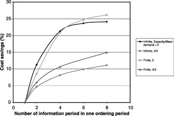
To understand the impact of the frequency of information sharing in the infinite time horizon case, in Figure 2 we display the percentage cost savings from information sharing as a function of the number of information periods in one ordering period, for both finite and infinite time horizon cases. The number of information periods, N, was two, four, six, and eight, whereas the length of the ordering period was assumed to be constant in all cases. The demand distribution during the entire ordering period is assumed to be Poisson with parameter λ = 24; hence, demand in a single information period is Poisson with parameter λ/N. Similarly, the inventory holding cost per ordering period is set up to be a constant $4 per unit product. Thus, the inventory holding cost per information period is 4/N, where N is the number of information periods within one ordering period. Total production capacity in the entire ordering period is kept constant and is equally divided among the different information periods. Finally, the ratio of penalty to holding costs is set to be 4.75 in all cases.

The impact of the frequency of information sharing.
Figure 2 implies that as the number of information periods increases, the percentage savings increase. However, the marginal benefit is a decreasing function of the number of information periods. Specifically, the additional benefit achieved by increasing the number of information periods from four to eight is relatively small. Finally, the difference between the cost savings obtained in finite and infinite time horizons is relatively small.
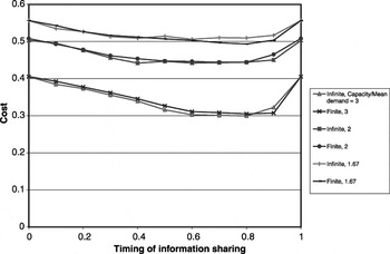
To understand the impact of the time when information is shared and the optimal timing of information sharing in infinite time horizon, we analyze the following case in which the retailer only shares demand information once with the manufacturer in one ordering period. In this case, we equally divide 1 ordering period into 10 intervals and compute the total cost for the manufacturer when the retailer shares demand information with her at one of these intervals.
Figure 3 presents the total cost of the manufacturer as a function of time when information is shared. Figure 3 provides normalized cost as a function of normalized time; that is, time is normalized and is measured from zero to one, while cost is normalized by hN NED, where ED is the expected demand in one information period. Thus, 0 in the x coordinate implies that information is shared at the beginning of an ordering period, and 1 means that information is shared at the end of an ordering period and hence cannot be used. Demand distribution is assumed to be Poisson(24) and the ratio of penalty to holding costs is 4.

The impact of the timing of information sharing for different levels of production capacity, i.i.d. demand.
Figure 3 implies that the optimal timing for information sharing is in the second half of the order interval. This is true both in the finite and infinite horizon models. Intuitively, when capacity is very large, it is appropriate to postpone the timing of information sharing to the last production opportunity in this ordering period; interestingly, this is also the right thing to do when capacity is tightly constrained (i.e., postpone the timing of information sharing until the last production opportunity). One possible explanation is that when capacity is very tight, the manufacturer needs to build as much inventory as she can until the last production opportunity, when she can review demand information and adjust production quantity.
5.2. Nonstationary Demand
In this subsection, we study the impact of independent but nonstationary demand on the benefits of information sharing in an infinite time horizon case. For this purpose, we first compare the percentage cost savings obtained in two systems: one facing i.i.d. demand and the other facing independent, nonstationary demand distributions. Then, we examine how nonstationary demand affects the optimal timing of information sharing.
To generate the nonstationary demand process, we modeled demand as a nonhomogenous Poisson process and considered the following two scenarios: piecewise increasing rate and piecewise decreasing demand rate.
In particular, demand follows Poisson(λ(t)) distribution for t ∈ [0,T] . The demand rate λ(t) is a piecewise constant simple function, and

, where Λ is the total average demand in one ordering period. Assuming that there are N information periods in one ordering period and λ(t) is a constant in every information period, we can write it as λ(n),n = 1,…,N.
Define dλ to be the difference between the highest demand rate and the lowest demand rate in one ordering period and let Δλ = [N/(N − 1)] dλ. Then, we determine the increasing λ(n) as follows:

The decreasing λ(n) can be determined by reversing the index of information periods. It is easily seen that λ(n) satisfies the condition

. To create a comparable i.i.d. demand distribution, we let the demand distribution be Poisson(Λ/N) in every information period.
To study the impact of nonstationary demand on cost savings, we show in Figure 4 the percentage cost saving from information sharing as a function of production capacity with increasing, decreasing, and i.i.d. demand. In all cases, N = 4 and each ordering period is equally divided into N information periods. We choose Λ = 20, Δλ = 6, and the ratio of penalty to inventory holding cost in one ordering period to be 4.75.

The impact of production capacity, non-i.i.d. demand.
Figure 4 illustrates that nonstationary demand has a significant impact on the benefit from information sharing. The percentage cost saving is the smallest when the demand rate is increasing, and it is the highest when the demand rate is decreasing for all production capacity levels. For instance, the difference between the percentage cost saving of increasing and decreasing demand rates is about 15% when the ratio of capacity to mean demand is 2.
This is quite intuitive because in the case of decreasing demand rate, realized demand in the first few information periods, on average, accounts for a larger portion of the total demand in one ordering period relative to increasing demand rate. Indeed, an extreme example of increasing demand rate is that demand is exactly zero in all information periods except the last one. In the last information period, demand equals the total demand in one ordering period. As we show in Section 5, this example is equivalent to a model with a no-information-sharing case. Similarly, an extreme example of the decreasing demand rate is that demand is exactly zero in all information periods except for the first one. In the first information period, demand equals the total demand in one ordering period and, hence, information has a significant impact on the manufacturer's cost.
To study the impact of nonstationary demand on the optimal timing of information sharing, we present in Figure 5 the manufacturer's cost as a function of the time when information is shared. The ratio of production capacity to mean demand in one ordering period is 2. We use the same settings as in Section 5.1 except that we allow for nonstationary demand distributions, where Λ = 30 and Δλ = 4.

The impact of the timing of information sharing, non-i.i.d. demand.
In Figure 6, we demonstrate the optimal timing of information sharing as a function of the production capacity in the cases of increasing and decreasing demand rates.

The impact of non-i.i.d. demand on the optimal timing of information sharing.
Figures 5 and 6 suggest the following observations:
[bull ] Information sharing is most beneficial in the case of decreasing demand rate and it is least beneficial in the case of increasing demand rate. Given that demand information is shared only once in one ordering period, the percentage cost saving in the case of decreasing demand rate can be as much as 17%, whereas it can only be as much as 11.3% in the case of increasing demand rate.
[bull ] Figures 5 and 6 show that demand information should always be shared earlier in the case of decreasing demand rate relative to increasing demand rate for different ratios of production capacity to mean demand. For example, when the ratio of capacity to mean demand equals 2 (Fig. 5), it is optimal to transfer demand information as early as 0.6 (in a scaled time horizon) in the case of decreasing demand rate, whereas in the case of increasing demand rate, the optimal timing of information sharing is as late as 0.8.
[bull ] This is quite intuitive because when demand rate is decreasing, most of the demand faced by the retailer is realized close to the beginning of the ordering period. On the other hand, when the demand rate is increasing, most demands are realized close to the end of the ordering period. Thus, it is better to share information earlier and leave more time for production in the decreasing demand rate case.
6. CONCLUSION
In this article, we analyze the value of information sharing in a two-stage supply chain with a single manufacturer and a single retailer. The manufacturer has finite production capacity and she receives demand information from the retailer even during periods of time in which the retailer does not make ordering decisions. A similar model is studied by Simchi-Levi and Zhao [28] in the finite time horizon case; the current article extends the analysis to the infinite time horizon case.
For this purpose, we first show that for any finite cyclic order-up-to policy, the associated inventory positions and shortfalls give rise to Markov chains with a single irreducible, positive recurrent class and a finite steady state average cost. The proof is based on the Foster's criterion and Lyapunov function, as well as a new method to relate Markov chains. This, together with the observation that the optimal policy under the discounted cost criterion can be characterized by a finite set of critical numbers, enables us to provide a simple proof for the optimality of cyclic order-up-to policy under the average cost criterion.
Interestingly, this approach can be applied to prove the existence of an optimal policy under the average cost criterion for other MDPs with unbounded costs. For this purpose, the optimal policy in these MDPs under the discounted cost criterion must be characterized by a finite set of critical numbers—for instance, inventory models with setup cost where the optimal policy under the discounted cost criterion is an (s,S) policy.
Using an extensive computational study, we demonstrate the potential benefits of information sharing on the manufacturer's cost and service level. In particular, we observe that the percentage cost savings due to information sharing increases as production capacity increases. This is true in both finite and infinite time horizon models. We also observe that nonstationary demand may have a substantial impact on both the benefits from information sharing and the optimal timing of information sharing. For instance, if the demand rate is increasing, the benefit from information sharing is not as high as that of decreasing demand rate.
APPENDIX
Proof of Proposition 3.1
Let us first consider the shortfall process {smN+n,m = 0,1,…} for n = 1,…,N. We start our proof by assuming i.i.d. demand D with mean ED. Without loss of generality, we assume initial state x0 ≤ 0, since states larger than zero are transient. Since

the shortfall process {st,n = 0,1,…} has state space S = {0,1,…} and transition function st = (st−1 + D − C)+. Thus, the transition matrix is

Let

. If i ≥ C,

If i < C,

So from Pakes' lemma (Kulkarni [20]), the shortfall process of order-up-to zero policy with i.i.d demand is positive recurrent if ED < C.
Assume that demands in different periods are independent of each other; the result can be easily extended to systems with periodical demand D1,D2,…,DN for any finite N (see Simchi-Levi and Zhao [29] for technical details).
The relationship between yt and st is st = −yt, and we also have xt+1 = min{0,xt + C} − Dt. The proofs of positive recurrence for xt and yt are similar.
Proof of Lemma 3.3
To prove the first part of the lemma, it is sufficient to show the existence of a Lyapunov function V satisfying the requirement of Lemma 3.2.
We start by analyzing i.i.d. demand D with mean ED. Let V(x) = qρ(x + C)ρ+1 and qρ = 1/(ρ + 1)(C − ED). Clearly, V(·) maps the state space of the shortfall S = {0,1,2,…} to R+.
If i ≥ C,

where

is the kth moment of demand. Further expanding the equation, we obtain

If i < C,

To summarize, in both cases,

where

Define the single-period cost function as

and since mk < +∞ for all positive integer k ≤ ρ + 1, then from Lemma 3.2 and Proposition 3.1, steady-state average cost is finite for the shortfall sn with single-period cost function rρ(x).
In fact, if the single period cost function is rl(x),∀0 < l < ρ, where

the same analysis shows that the corresponding steady state average cost is finite for the shortfall sn.
Finally, our objective is to show that if the single period cost function is xl, then the steady state average cost of the shortfall is finite. For this purpose, we use induction on l. The case l = 1 is obvious since we already know that for r1(x) = x, the steady-state average cost is finite. By induction on l and the fact that steady-state average cost of the shortfall is finite for rl(x), 0 < l < ρ, we obtain our result.
We can extend the result to independent demand with periodically varying distributions D1,D2,…,DN in a similar way by defining

. We omit the proof and refer the readers to Simchi-Levi and Zhao [29] for technical details.
We now prove the second part of the lemma. Since st is nonnegative, the monotone convergence theorem implies that
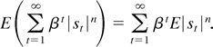
Because of the first part of this lemma and 0 < β < 1, this summation is for a power series with positive and bounded coefficients, so it is finite.
Since the inventory position processes yt = −st and xt+1 = yt − Dt, it is easy to show that the same arguments hold for yt and xt. █
Footnotes
Research supported in part by ONR contracts N00014-95-1-0232 and N00014-01-1-0146 and NSF contracts DMI-9732795, DMI-0085683, and DMI-0245352.
References
REFERENCES
Aviv, Y. &
Federgruen, A.
(1997).
Stochastic inventory models with limited production capacities and
periodically varying parameters.
Probability in the Engineering and Informational Sciences
11:
107–135.Google Scholar
Aviv, Y. &
Federgruen, A.
(1998).
The operational benefits of information sharing and vendor managed
inventory (VMI) programs.
Working Paper.
Washington University,
St. Louis.
Cachon, G.P. &
Fisher, M.
(2000).
Supply chain inventory management and the value of shared
information.
Management Science
46:
1032–1050.Google Scholar
Chen, F.
(1998).
Echelon reorder points, installation reorder points, and the value
of centralized demand information.
Management Science
44:
221–234.Google Scholar
Chen, F.,
Drezner, I.,
Ryan, J.K., &
Simchi-Levi, D.
(2000).
Quantifying the bullwhip effect in a simple supply chain: The
impact of forecasting, lead time, and information.
Management Science
46:
436–443.Google Scholar
Federgruen, A.,
Schweitzer, P., &
Tijms, H.
(1983).
Denumerable undiscounted decision processes with unbounded rewards.
Mathematics of Operations Research
8:
298–314.Google Scholar
Federgruen, A. &
Zipkin, P.
(1986).
An inventory model with limited production capacity and uncertain
demands 1: The average-cost criterion.
Mathematics of Operations Research
11:
193–207.Google Scholar
Federgruen, A. &
Zipkin, P.
(1986).
An inventory model with limited production capacity and uncertain
demands 2: The discounted-cost criterion.
Mathematics of Operations Research
11:
208–215.Google Scholar
Fu, M.C.
(1994).
Optimization via simulation: A review.
Annals of Operations Research
53:
199–247.Google Scholar
Gallego, G. &
Ozer, O.
(2001).
Integrating replenishment decisions with advanced demand
information.
Management Science
47:
1344–1360.Google Scholar
Gavirneni, S.,
Kapuscinski, R., &
Tayur, S.
(1999).
Value of information in capacitated supply chains.
Management Science
45:
16–24.Google Scholar
Glasserman, P. &
Tayur, S.
(1995).
Sensitivity analysis for base-stock levels in multiechelon
production-inventory systems.
Management Science
41:
263–281.Google Scholar
Hariharan, R. &
Zipkin, P.
(1995).
Customer-order information, lead times, and inventories.
Management Science
41:
1599–1607.Google Scholar
Heyman, D. &
Sobel, M.
(1984).
Stochastic models in operations research,
Vol. 2.
New York:
McGraw-Hill.
Kapuscinski, R. &
Tayur, S.
(1995).
A capacitated production–inventory model with periodic
demand.
GSIA Working Paper.
Carnegie Mellon University,
Pittsburgh, PA.
Kapuscinski, R. &
Tayur, S.
(1998).
A capacitated production-inventory model with periodic demand.
Operations Research
46:
899–911.Google Scholar
Karlin, S.
(1960).
Dynamic inventory policy with varying stochastic demands.
Management Science
6:
231–258.Google Scholar
Karr, A.F.
(1993).
Probability.
New York:
Springer-Verlag.
Kemeny, J.G.,
Snell, J.L., &
Knapp, A.W.
(1966).
Denumerable Markov chains.
New York:
D. Van Nostrand.
Kulkarni, V.G.
(1995).
Modeling and analysis of stochastic systems.
New York:
Chapman & Hall.
Lee, H.,
Padmanabhan, P., &
Whang, S.
(1997).
Information distortion in a supply chain: The Bullwhip effect.
Management Science
43:
546–558.Google Scholar
Lee, H.,
So, K.C., &
Tang, C.S.
(2000).
The value of information sharing in a two-level supply chain.
Management Science
46:
626–643.Google Scholar
Meyn, S.P. &
Tweedie, R.L.
(1993).
Markov chains and stochastic stability.
London:
Springer-Verlag.
Puterman, M.L.
(1994).
Markov decision processes: Discrete stochastic dynamic programming.
New York:
Wiley.
Sennott, L.I.
(1989).
Average cost optimal stationary policies in infinite state Markov
decision processes with unbounded costs.
Operations Research
37:
261–272.Google Scholar
Sennott, L.I.
(1999).
Stochastic dynamic programming and the control of queuing systems.
New York:
Wiley.
Sethi, S.P. &
Cheng, F.
(1997).
Optimality of (s,S) policies in inventory models with Markovian
demand.
Operations Research
45:
931–939.Google Scholar
Simchi-Levi, D. &
Zhao, Y.
(to appear).
The value of information sharing in a two-stage supply chain with
production capacity constraints.
Naval Research Logistics;
available upon request from yaozhao@andromeda.rutgers.edu.
Simchi-Levi, D. &
Zhao, Y.
(2001).
The value of information sharing in a two-stage supply chain with
production capacity constraints: The infinite horizon case.
Working Paper.
Rutgers University,
Newark, NJ;
available upon request from yaozhao@andromeda.rutgers.edu.
Song, J.S. &
Zipkin, P.
(1993).
Inventory control in a fluctuating environment.
Operations Research
41:
351–370.Google Scholar
Stein, T. &
Sweat, J.
(1998).
Killer supply chains.
Information Week.
Obtained at www.informationweek.com/708/08iukil.htm.
Zipkin, P.
(1989).
Critical number policies for inventory models with periodic data.
Management Science
35:
71–80.Google Scholar
The impact of the production capacity, i.i.d. demand.
The impact of the frequency of information sharing.
The impact of the timing of information sharing for different levels of production capacity, i.i.d. demand.
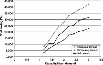
The impact of production capacity, non-i.i.d. demand.
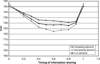
The impact of the timing of information sharing, non-i.i.d. demand.
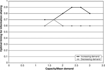
The impact of non-i.i.d. demand on the optimal timing of information sharing.
 You have
Access
- 13
- Cited by