2.1 Description of the local scattering problem

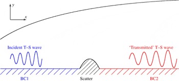
A typical local scattering problem is illustrated in figure 1 for the specific case of an isolated roughness element on an otherwise flat plate (Wu & Hogg Reference Wu and Hogg2006; Wu & Dong Reference Wu and Dong2016). In general, the two flat portions of the boundaries are punctuated by a relatively small region of rapid variation, which causes short streamwise inhomogeneity. An oncoming (incident) instability mode, originated from the flat portion upstream (referred to as BC1), approaches the site of the local change and is scattered by the streamwise inhomogeneity. In the region far downstream of the scatter (referred to as BC2), the disturbance relaxes to a local eigenmode, which will be referred to as the transmitted wave. Typical scatters include the following.

Figure 1.

A diagrammatic illustration of a local scattering problem.

1. (i) Local roughness/wavy surface (Nayfeh et al. Reference Nayfeh, Ragab and Almaaitah1988; Cebeci & Egan Reference Cebeci and Egan1989; Fujii Reference Fujii2006)

   BC1/BC2 before/after the scatter are both rigid flat walls, between which a local roughness element is present. The shape of the roughness, $y=hF((x-x_{c})/d)$ , changes over on the scale $d$ , which is assumed to be comparable with the wavelength, where $x_{c}$ denotes the location of the roughness centre.

2. (ii) Local suction/injection or heating/cooling on the wall (Nayfeh & Reed Reference Nayfeh and Reed1985; Reed & Nayfeh Reference Reed and Nayfeh1986; Reynolds & Saric Reference Reynolds and Saric1986; Masad & Nayfeh Reference Masad and Nayfeh1992; Masad Reference Masad1995)

   BC1 and BC2 are both rigid walls, and a steady suction/injection with a wall-normal velocity $\bar{v}((x-x_{c})/d)$ or surface heating/cooling with a temperature $\bar{T}((x-x_{c})/d)$ , is applied on a finite section, whose length $d$ is comparable with the wavelength.

3. (iii) Local porous/flexible surfaces (Wang & Zhong Reference Wang and Zhong2012)

   BC1 and BC2 are both rigid walls, and they are joined by a porous or compliant section, where the unsteady normal velocity $v^{\prime }$ , or the wall displacement $f^{\prime }$ , is related to the pressure fluctuation $p^{\prime }$ on the surface.

4. (iv) Junction of a rigid wall with a semi-infinite porous/flexible surface

   BC1 is a rigid wall, while BC2 is a porous/flexible surface or vice versa. Here BC2 extends to infinity so that the junction acts a scatter.

We shall assume that (i) the base flow is steady, and the unsteady fluctuation is of small amplitude so that the linearized disturbance equations are valid in the whole domain and (ii) the scatter is local, whose width $d$ in the streamwise direction is comparable with the characteristic wavelength of the instability of the unperturbed flow. It follows that even though the disturbances far upstream and downstream are local eigenmodes, the fluctuation near the scatter is not and can indeed be rather complex.

Figure 2.

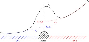
A diagrammatic illustration of local scattering and transmission coefficient $Tr=A_{T}(x_{c})/A_{I}(x_{c})$ , where $x_{c}$ is the centre of the scatter, $A_{s}$ the amplitude of disturbance in the presence of the scatter, whereas $A_{I}$ and $A_{T}$ represent the evolution and extrapolation of the incident and transmitted waves respectively in the absence of a scatter.

The impact of these abrupt distortions on instability and transition will be investigated in the framework of LSA, the key concept of which is the transmission coefficient (Wu & Hogg Reference Wu and Hogg2006). Its definition is illustrated in figure 2. Suppose that an incident instability wave, with an initial amplitude $A_{0}$ at position $x_{0}$ say, propagates downstream. Sufficiently upstream of the roughness element centred at $x_{c}$ , the amplitude $A_{s}$ of the instability wave evolves according to LST (as indicated by the dotted line), but in the vicinity of the roughness $A_{s}$ deviates from that predicted by LST, and follows instead the solid curve in the figure. Sufficiently downstream, the disturbance relaxes to a local instability mode and is thus referred to as the transmitted instability wave. Let $A_{n}$ denote the amplitude at position $x_{n}$ and $\unicode[STIX]{x1D6FC}_{T}$ denote the local eigenvalue in the far downstream region in the absence of the scatter (a region of rapid variation or a junction). Using $A_{n}$ and $\unicode[STIX]{x1D6FC}_{T}$ , one may extrapolate an effective initial amplitude $A_{T}(x_{c})$ at  $x_{c}$ ,

(2.1) $$\begin{eqnarray}A_{T}(x_{c})=A_{n}\exp \left\{-\text{i}\int _{x_{c}}^{x_{n}}\unicode[STIX]{x1D6FC}_{T}(x)\,\text{d}x\right\},\end{eqnarray}$$

which is referred to as the amplitude of the transmitted wave. Note however that $A_{T}(x_{c})$ is not the amplitude of the physical disturbance at $x_{c}$ , i.e.  $A_{T}(x_{c})\neq A_{s}(x_{c})$ , but it is $A_{T}(x_{c})$ that is important and relevant as will become clear later. On the other hand, if the scatter were absent, the upstream instability mode would have evolved according to LST (indicated by the dotted line in figure 2) to acquire an amplitude at  $x_{c}$ ,

(2.2) $$\begin{eqnarray}A_{I}(x_{c})=A_{0}\exp \left\{\text{i}\int _{x_{0}}^{x_{c}}\unicode[STIX]{x1D6FC}_{I}(x)\,\text{d}x\right\},\end{eqnarray}$$

where $\unicode[STIX]{x1D6FC}_{I}$ denotes the local eigenvalue in the far upstream region in the absence of the scatter and $A_{I}(x_{c})$ defines the ‘amplitude of the incident wave’.

The transmission coefficient is then defined as (Wu & Hogg Reference Wu and Hogg2006)

(2.3) $$\begin{eqnarray}Tr=A_{T}(x_{c})/A_{I}(x_{c}).\end{eqnarray}$$

In the absence of a scatter, $A_{T}(x_{c})=A_{I}(x_{c})$ . It follows that the transmission coefficient provides a natural characterization of the impact of the scatter on stability and transition: the scatter suppresses the instability wave and hence delays transition if $|Tr|<1$ , but enhances the instability wave and boosts transition if $|Tr|>1$ .

The introduction of $Tr$ based on $A_{T}(x_{c})$ is convenient because it encapsulates the effect of the scatter and thereby allows LSA to be linked naturally with existing transition prediction methods for canonical boundary layers as follows. Use LST or PSE to describe the evolution of the instability wave upstream of the scatter and to obtain $A_{I}(x_{c})$ . Then using $Tr$ , one finds $A_{T}(x_{c})=Tr\,A_{I}(x_{c})$ . With this $A_{T}(x_{c})$ as the initial condition, LST or PSE can again be employed to predict the equivalent development far downstream of the scatter. With the aid of $Tr$ , the development of the disturbance in the presence of a scatter is converted into an equivalent one without the scatter.

Before presenting a detailed mathematical formulation of LSA, we first highlight its key features and the main difference from LST and PSE. As in previous studies (Wu & Hogg Reference Wu and Hogg2006; Wu & Dong Reference Wu and Dong2016), it suffices to consider a wave with a given frequency $\unicode[STIX]{x1D714}$ since the disturbance is assumed to be small. We may write $\boldsymbol{Q}^{\prime }$ in the form

(2.4) $$\begin{eqnarray}\boldsymbol{Q}^{\prime }(x,y,t)=\boldsymbol{q}(x,y)\exp (-\text{i}\unicode[STIX]{x1D714}t)+\text{c.c.}\end{eqnarray}$$

It is important to point out that unlike the shape function (1.2) or (1.5) in LST and PSE respectively, the streamwise variation of $\boldsymbol{q}$ in (2.4) is on the short scale, comparable with the wavelength of the oncoming instability mode. Substituting (2.4) into the N–S equations and linearizing about the steady base flow, we obtain the equations for $\boldsymbol{q}(x,y)$ , which form, along with appropriate boundary conditions including the upstream and downstream conditions, a boundary-value problem that is elliptic in its nature. The ansatz (2.4) looks similar to that in global stability analysis in that both allow for fast variation with  $x$ . The differences and relation between the two are worth noting. The first difference is that the frequency $\unicode[STIX]{x1D714}$ in the present work is real and given, as opposed to being a generally complex-valued eigenvalue to be found in the global stability problem. The second difference is that discrete global modes are usually assumed to be localized, i.e. attenuate in both the upstream and downstream directions, while the disturbances in the present scattering problem amplify downstream. On the basis of the last observation, the disturbance in the scattering problem may be viewed as a continuous neutral global mode.

For instability modes of the T–S type, the frequency $\unicode[STIX]{x1D714}\neq 0$ . However, we may set $\unicode[STIX]{x1D714}=0$ in the formulation if time-independent instability waves are considered, such as stationary cross-flow vortices arising in three-dimensional boundary layers subject to a pressure gradient. Scattering of pre-existing vortices by two- and/or three-dimensional scatters can be analysed in the same framework. Furthermore, by setting the amplitude of the upstream mode to zero ( $A_{I}=0$ ), the mathematical framework may also be used to compute the amplitude of the cross-flow vortices excited by streamwise compact and spanwise periodic roughness elements (Choudhari & Duck Reference Choudhari, Duck, Duck and Philip1996; Kurz & Kloker Reference Kurz and Kloker2014).

2.2 Governing equations

The formulation of LSA will be given for a general three-dimensional incompressible boundary layer that develops over a nominally flat surface. The flow is described in the Cartesian coordinates $(x^{\ast },y^{\ast },z^{\ast })$ , in which the surface is located at $y^{\ast }=0$ with its leading edge at $x^{\ast }=0$ and the $x^{\ast }$ axis pointing to the downstream direction, while $z^{\ast }$ is in the spanwise direction. Let $U_{\infty }^{\ast },\unicode[STIX]{x1D70C}_{\infty }^{\ast }$ and $\unicode[STIX]{x1D707}_{\infty }^{\ast }$ denote the free-scream velocity, density and viscous coefficient respectively with the superscript $\ast$ indicating a dimensional quantity. The reference length and time are taken to be $\unicode[STIX]{x1D6FF}^{\ast }$ and $\unicode[STIX]{x1D6FF}^{\ast }/U_{\infty }^{\ast }$ respectively, where $\unicode[STIX]{x1D6FF}^{\ast }$ is the displacement thickness of the boundary layer at a typical streamwise location. The resulting dimensionless coordinates and time variable will be denoted as $(x,y,z)$ and $t$ respectively. The velocity and pressure are normalized by $U_{\infty }^{\ast }$ and $\unicode[STIX]{x1D70C}_{\infty }^{\ast }U_{\infty }^{\ast 2}$ respectively, and the corresponding non-dimensional quantities are denoted by $(u,v,w)$ and  $p$ . The dimensionless three-dimensional incompressible N–S equations read

(2.5) $$\begin{eqnarray}\displaystyle & \displaystyle \frac{\unicode[STIX]{x2202}u}{\unicode[STIX]{x2202}x}+\frac{\unicode[STIX]{x2202}v}{\unicode[STIX]{x2202}y}+\frac{\unicode[STIX]{x2202}w}{\unicode[STIX]{x2202}z}=0, & \displaystyle\end{eqnarray}$$

(2.6) $$\begin{eqnarray}\displaystyle & \displaystyle \frac{\unicode[STIX]{x2202}u}{\unicode[STIX]{x2202}t}+u\frac{\unicode[STIX]{x2202}u}{\unicode[STIX]{x2202}x}+v\frac{\unicode[STIX]{x2202}u}{\unicode[STIX]{x2202}y}+w\frac{\unicode[STIX]{x2202}u}{\unicode[STIX]{x2202}z}=-\frac{\unicode[STIX]{x2202}p}{\unicode[STIX]{x2202}x}+\frac{1}{R}\left(\frac{\unicode[STIX]{x2202}^{2}u}{\unicode[STIX]{x2202}x^{2}}+\frac{\unicode[STIX]{x2202}^{2}u}{\unicode[STIX]{x2202}y^{2}}+\frac{\unicode[STIX]{x2202}^{2}u}{\unicode[STIX]{x2202}z^{2}}\right), & \displaystyle\end{eqnarray}$$

(2.7) $$\begin{eqnarray}\displaystyle & \displaystyle \frac{\unicode[STIX]{x2202}v}{\unicode[STIX]{x2202}t}+u\frac{\unicode[STIX]{x2202}v}{\unicode[STIX]{x2202}x}+v\frac{\unicode[STIX]{x2202}v}{\unicode[STIX]{x2202}y}+w\frac{\unicode[STIX]{x2202}v}{\unicode[STIX]{x2202}z}=-\frac{\unicode[STIX]{x2202}p}{\unicode[STIX]{x2202}y}+\frac{1}{R}\left(\frac{\unicode[STIX]{x2202}^{2}v}{\unicode[STIX]{x2202}x^{2}}+\frac{\unicode[STIX]{x2202}^{2}v}{\unicode[STIX]{x2202}y^{2}}+\frac{\unicode[STIX]{x2202}^{2}v}{\unicode[STIX]{x2202}z^{2}}\right), & \displaystyle\end{eqnarray}$$

(2.8) $$\begin{eqnarray}\displaystyle & \displaystyle \frac{\unicode[STIX]{x2202}w}{\unicode[STIX]{x2202}t}+u\frac{\unicode[STIX]{x2202}w}{\unicode[STIX]{x2202}x}+v\frac{\unicode[STIX]{x2202}w}{\unicode[STIX]{x2202}y}+w\frac{\unicode[STIX]{x2202}w}{\unicode[STIX]{x2202}z}=-\frac{\unicode[STIX]{x2202}p}{\unicode[STIX]{x2202}z}+\frac{1}{R}\left(\frac{\unicode[STIX]{x2202}^{2}w}{\unicode[STIX]{x2202}x^{2}}+\frac{\unicode[STIX]{x2202}^{2}w}{\unicode[STIX]{x2202}y^{2}}+\frac{\unicode[STIX]{x2202}^{2}w}{\unicode[STIX]{x2202}z^{2}}\right), & \displaystyle\end{eqnarray}$$

where $R$ is the Reynolds number, defined as

(2.9) $$\begin{eqnarray}R=\unicode[STIX]{x1D70C}_{\infty }^{\ast }U_{\infty }^{\ast }\unicode[STIX]{x1D6FF}^{\ast }/\unicode[STIX]{x1D707}_{\infty }^{\ast }.\end{eqnarray}$$

2.3 Linearized perturbation equations

Let $\bar{\boldsymbol{Q}}(x,y)$ denote the three-dimensional base-flow field. When it is perturbed by a small-amplitude disturbance $\boldsymbol{Q}^{\prime }(x,y,z,t)$ , the total flow field $\boldsymbol{Q}(x,y,z,t)$ is written as

(2.10) $$\begin{eqnarray}\displaystyle \boldsymbol{Q}=(u,v,w,p) & = & \displaystyle (\bar{u}(x,y),\bar{v}(x,y),\bar{w}(x,y),\bar{p}(x,y))+(u^{\prime },v^{\prime },w^{\prime },p^{\prime })\nonumber\\ \displaystyle & \equiv & \displaystyle \bar{\boldsymbol{Q}}(x,y)+\boldsymbol{Q}^{\prime }(x,y,z,t).\end{eqnarray}$$

Substituting (2.10) into (2.5)–(2.8), and linearizing about the base flow, we obtain the linear N–S equations for the perturbation. For the ensuing analysis, it is convenient to cast them into the matrix form,

(2.11) $$\begin{eqnarray}\left[\tilde{\unicode[STIX]{x1D63C}}+\tilde{\unicode[STIX]{x1D63D}}_{1}\frac{\unicode[STIX]{x2202}}{\unicode[STIX]{x2202}x}+\tilde{\unicode[STIX]{x1D63D}}_{2}\frac{\unicode[STIX]{x2202}}{\unicode[STIX]{x2202}y}+\tilde{\unicode[STIX]{x1D63D}}_{3}\frac{\unicode[STIX]{x2202}}{\unicode[STIX]{x2202}z}+\tilde{\unicode[STIX]{x1D63E}}\left(-R\frac{\unicode[STIX]{x2202}}{\unicode[STIX]{x2202}t}+\frac{\unicode[STIX]{x2202}^{2}}{\unicode[STIX]{x2202}x^{2}}+\frac{\unicode[STIX]{x2202}^{2}}{\unicode[STIX]{x2202}y^{2}}+\frac{\unicode[STIX]{x2202}^{2}}{\unicode[STIX]{x2202}z^{2}}\right)\right]\boldsymbol{Q}^{\prime }=\mathbf{0},\end{eqnarray}$$

where we have put

(2.12a,b ) $$\begin{eqnarray}\tilde{\unicode[STIX]{x1D63C}}(x,y)=\left[\begin{array}{@{}cccc@{}}0 & 0 & 0 & 0\\ \unicode[STIX]{x2202}\bar{u}/\unicode[STIX]{x2202}x & \unicode[STIX]{x2202}\bar{u}/\unicode[STIX]{x2202}y & 0 & 0\\ \unicode[STIX]{x2202}\bar{v}/\unicode[STIX]{x2202}x & \unicode[STIX]{x2202}\bar{v}/\unicode[STIX]{x2202}y & 0 & 0\\ \unicode[STIX]{x2202}\bar{w}/\unicode[STIX]{x2202}x & \unicode[STIX]{x2202}\bar{w}/\unicode[STIX]{x2202}y & 0 & 0\end{array}\right],\quad \tilde{\unicode[STIX]{x1D63D}}_{1}(x,y)=\left[\begin{array}{@{}cccc@{}}1 & 0 & 0 & 0\\ \bar{u} & 0 & 0 & 1\\ 0 & \bar{u} & 0 & 0\\ 0 & 0 & \bar{u} & 0\end{array}\right],\end{eqnarray}$$

(2.13a-c ) $$\begin{eqnarray}\tilde{\unicode[STIX]{x1D63D}}_{2}=\left[\begin{array}{@{}cccc@{}}0 & 1 & 0 & 0\\ \bar{v} & 0 & 0 & 0\\ 0 & \bar{v} & 0 & 1\\ 0 & 0 & \bar{v} & 0\end{array}\right],\quad \tilde{\unicode[STIX]{x1D63D}}_{3}=\left[\begin{array}{@{}cccc@{}}0 & 0 & 1 & 0\\ \bar{w} & 0 & 0 & 0\\ 0 & \bar{w} & 0 & 0\\ 0 & 0 & \bar{w} & 1\end{array}\right],\quad \tilde{\unicode[STIX]{x1D63E}}=-\frac{1}{R}\left[\begin{array}{@{}cccc@{}}0 & 0 & 0 & 0\\ 1 & 0 & 0 & 0\\ 0 & 1 & 0 & 0\\ 0 & 0 & 1 & 0\end{array}\right].\end{eqnarray}$$

Since the base flow is steady and uniform in the spanwise direction, the perturbation $\boldsymbol{Q}^{\prime }(x,y,z,t)$ can be written as

(2.14) $$\begin{eqnarray}\boldsymbol{Q}^{\prime }(x,y,z,t)=\unicode[STIX]{x1D719}(x,y)\exp [\text{i}(\unicode[STIX]{x1D6FD}z-\unicode[STIX]{x1D714}t)]+\text{c.c.},\end{eqnarray}$$

where $\unicode[STIX]{x1D714}$ and $\unicode[STIX]{x1D6FD}$ are real constants and the shape function $\unicode[STIX]{x1D719}(x,y)$ depends on $x$ and  $y$ . Substitution of (2.14) into (2.11) yields the equations governing  $\unicode[STIX]{x1D719}$ ,

(2.15) $$\begin{eqnarray}\hat{\unicode[STIX]{x1D63C}}\unicode[STIX]{x1D719}+\hat{\unicode[STIX]{x1D63D}}\frac{\unicode[STIX]{x2202}\unicode[STIX]{x1D719}}{\unicode[STIX]{x2202}x}+\hat{\unicode[STIX]{x1D63E}}\frac{\unicode[STIX]{x2202}^{2}\unicode[STIX]{x1D719}}{\unicode[STIX]{x2202}x^{2}}=\mathbf{0},\end{eqnarray}$$

where

(2.16a,b ) $$\begin{eqnarray}\unicode[STIX]{x1D719}(x,y)=\left[\begin{array}{@{}c@{}}\hat{u} \\ \hat{v}\\ {\hat{w}}\\ \hat{p}\end{array}\right],\quad \hat{\unicode[STIX]{x1D63C}}(x,y)=\left[\begin{array}{@{}cccc@{}}0 & D & \text{i}\unicode[STIX]{x1D6FD} & 0\\ \unicode[STIX]{x2202}\bar{u}/\unicode[STIX]{x2202}x+s & \unicode[STIX]{x2202}\bar{u}/\unicode[STIX]{x2202}y & 0 & 0\\ \unicode[STIX]{x2202}\bar{v}/\unicode[STIX]{x2202}x & \unicode[STIX]{x2202}\bar{v}/\unicode[STIX]{x2202}y+s & 0 & D\\ \unicode[STIX]{x2202}\bar{w}/\unicode[STIX]{x2202}x & \unicode[STIX]{x2202}\bar{w}/\unicode[STIX]{x2202}y & s & \text{i}\unicode[STIX]{x1D6FD}\end{array}\right],\end{eqnarray}$$

(2.17a,b ) $$\begin{eqnarray}\hat{\unicode[STIX]{x1D63D}}(x,y)=\left[\begin{array}{@{}cccc@{}}1 & 0 & 0 & 0\\ \bar{u} & 0 & 0 & 1\\ 0 & \bar{u} & 0 & 0\\ 0 & 0 & \bar{u} & 0\end{array}\right],\quad \hat{\unicode[STIX]{x1D63E}}=-\frac{1}{R}\left[\begin{array}{@{}cccc@{}}0 & 0 & 0 & 0\\ 1 & 0 & 0 & 0\\ 0 & 1 & 0 & 0\\ 0 & 0 & 1 & 0\end{array}\right],\end{eqnarray}$$

with

(2.18) $$\begin{eqnarray}s=\bar{v}D+\text{i}\unicode[STIX]{x1D6FD}\bar{w}-\text{i}\unicode[STIX]{x1D714}-[D^{2}+(\text{i}\unicode[STIX]{x1D6FD})^{2}]/R,\quad D=\unicode[STIX]{x2202}/\unicode[STIX]{x2202}y.\end{eqnarray}$$

Note that no assumption is made of the slow variation with $x$ of either the base flow or the perturbation.

2.4 Boundary conditions

2.4.1 Boundary conditions on the wall and at infinity

The abrupt change is created through the boundary conditions at the wall. We consider first the case associated with an abrupt change of wall porosity: a finite section of porous plate joining two rigid sections. A general theory for the flow through a porous medium does not exist. We shall adopt the model based on the Darcy’s law (Darcy Reference Darcy1856), which asserts that the velocity $v^{\ast }$ is proportional to the pressure gradient driving the flow, namely,

(2.19) $$\begin{eqnarray}v^{\ast }=-\frac{\unicode[STIX]{x1D705}^{\ast }}{\unicode[STIX]{x1D707}^{\ast }b^{\ast }}(p_{+}^{\ast }-p_{-}^{\ast }),\end{eqnarray}$$

where $\unicode[STIX]{x1D705}^{\ast }$ is the permeability of the medium, $\unicode[STIX]{x1D707}^{\ast }$ the dynamic viscosity of the fluid, $b^{\ast }$ the thickness of the layer of the porous medium and $(p_{+}^{\ast }-p_{-}^{\ast })$ represents the pressure difference across the medium. Typical intrinsic permeability $\unicode[STIX]{x1D705}^{\ast }$ ranges, in the unit of $\text{m}^{2}$ , from $10^{-10}$ to $10^{-7}$ for pervious media, from $10^{-14}$ to $10^{-11}$ for semi-pervious media and from $10^{-19}$ to $10^{-15}$ for impervious media (http://en.wikipedia.org/wiki/Permeability_(fluid)).

The fluid motion may not respond to the pressure instantaneously as is implied in (2.19). A simple model that accounts for this inertial effect results from adding an extra term $\unicode[STIX]{x1D706}_{2}^{\ast }\unicode[STIX]{x2202}v^{\ast }/\unicode[STIX]{x2202}t^{\ast }$ to (2.19) with $\unicode[STIX]{x1D706}_{2}^{\ast }$ being the relaxation time. When non-dimensionalized, the model for a porous wall reads

(2.20) $$\begin{eqnarray}\unicode[STIX]{x1D706}_{2}\frac{\unicode[STIX]{x2202}v}{\unicode[STIX]{x2202}t}+v=-\unicode[STIX]{x1D706}_{1}p,\end{eqnarray}$$

where we have set $p_{-}^{\ast }=0$ without losing generality, and the dimensionless parameters

(2.21a,b ) $$\begin{eqnarray}\unicode[STIX]{x1D706}_{1}=\frac{\unicode[STIX]{x1D705}^{\ast }}{\unicode[STIX]{x1D707}^{\ast }b^{\ast }}\unicode[STIX]{x1D70C}_{\infty }^{\ast }U_{\infty }^{\ast }=\frac{\unicode[STIX]{x1D705}^{\ast }}{b^{\ast }}Re^{\ast },\quad \unicode[STIX]{x1D706}_{2}=\unicode[STIX]{x1D706}_{2}^{\ast }U_{\infty }/\unicode[STIX]{x1D6FF}^{\ast }.\end{eqnarray}$$

For a unit Reynolds number $Re^{\ast }\approx 10^{6}~\text{m}^{-1}$ and a thickness $b^{\ast }\approx 10^{-2}~\text{m}$ , the range of $\unicode[STIX]{x1D706}_{1}$ for pervious media is from $10^{-2}$ to 10. In spectral space, equation (2.20) can be written as $-\text{i}\unicode[STIX]{x1D714}\unicode[STIX]{x1D706}_{2}\hat{v}+\hat{v}=-\unicode[STIX]{x1D706}_{1}\hat{p}$ , or

(2.22) $$\begin{eqnarray}\hat{v}=-\unicode[STIX]{x1D706}\hat{p}\quad \text{with}~\unicode[STIX]{x1D706}=\frac{\unicode[STIX]{x1D706}_{1}}{1-\text{i}\unicode[STIX]{x1D714}\unicode[STIX]{x1D706}_{2}},\end{eqnarray}$$

indicating that $\unicode[STIX]{x1D706}_{2}$ can be absorbed into $\unicode[STIX]{x1D706}$ by allowing the latter to take complex values.

At the wall ( $y=0$ ), three boundary conditions are therefore imposed, namely,

(2.23a,b ) $$\begin{eqnarray}\hat{u} (x,0)={\hat{w}}(x,0)=0,\quad \hat{v}(x,0)=\left\{\begin{array}{@{}ll@{}}-\unicode[STIX]{x1D706}\hat{p}, & x_{s}<x<x_{e},\\ 0 & \text{otherwise},\end{array}\right.\end{eqnarray}$$

where the first two correspond to the no-slip condition, and $(x_{s},x_{e})$ indicates the extent of the porous panel.

For the case of a local steady suction, an inhomogeneous boundary condition is imposed on the steady transverse velocity (see later), but the unsteady perturbation satisfies homogeneous boundary conditions, $\hat{u} ={\hat{w}}=0$ and $\hat{v}=0$ , with inhomogeneity appearing in the coefficients of its governing equations. The condition $\hat{v}=0$ can be considered as corresponding to $\unicode[STIX]{x1D706}_{1}(x)=\unicode[STIX]{x1D706}_{2}(x)=0$ , and it follows that the boundary conditions are also given by (2.23) provided that we set $\unicode[STIX]{x1D706}=0$ . Note that the suction of interest for us is completely different from that considered in some previous studies (Pralits, Hanifi & Henningson Reference Pralits, Hanifi and Henningson2002; Airiau et al. Reference Airiau, Bottaro, Walther and Legendre2003; Pralits & Hanifi Reference Pralits and Hanifi2003), where the suction is imposed over the long length scale comparable with the distances to the leading edge, and its magnitude is of $O(R^{-1}U_{\infty }\ast )$ . There the resulting steady flow is described by the classical boundary-layer theory, and the instability waves developing on the slowly evolving base flow are described by PSE or LST. The local suction in the present paper occurs on a sufficiently short scale that both the steady base flow and unsteady disturbances exhibit full ellipticity. The aim of our work is to develop an approach that would supersede LST and PSE.

It should be stressed that while the oncoming instability wave is assumed to be of small amplitude, the sudden variations have not been assumed small at all. They either alter the base flow by $O(1)$ amount as in the case of a local suction, or produce an $O(1)$ abrupt change of the boundary conditions as in the cases of a finite porous panel and a rigid–porous junction. In either form, the rapid variation exerts an $O(1)$ influence on the amplitude of the oncoming instability wave.

At infinity, the perturbation vanishes, namely

(2.24) $$\begin{eqnarray}(\hat{u} ,\hat{v},{\hat{w}},\hat{p})\rightarrow (0,0,0,0)\quad \text{as}~y\rightarrow \infty .\end{eqnarray}$$

2.4.2 The upstream and downstream conditions: incident and transmitted waves

In this paper, we will formulate LSA for abrupt isolated distortions neglecting the much weaker non-parallelism of the unperturbed base flow, an approximation consistent with that made in the high-Reynolds-number theory (Wu & Dong Reference Wu and Dong2016) and justifiable by the latter.

In LSP, an incident wave is imposed upstream. For a localized scatter at  $x_{c}$ , the disturbance far upstream and downstream takes the form of a local eigenmode, that is,

(2.25) $$\begin{eqnarray}\unicode[STIX]{x1D719}\rightarrow \tilde{\unicode[STIX]{x1D719}}(x,y)\exp \left\{\text{i}\int ^{x}\unicode[STIX]{x1D6FC}(x)\,\text{d}x\right\}+\text{c.c.}\quad \text{as}~x-x_{c}\rightarrow \pm \infty ,\end{eqnarray}$$

where $\unicode[STIX]{x1D6FC}(x)$ is the local streamwise wavenumber and $\tilde{\unicode[STIX]{x1D719}}(x,y)$ the corresponding eigenfunction. Under the local parallel-flow assumption, the streamwise variations of the base flow $\bar{\boldsymbol{Q}}$ and the eigenfunction $\tilde{\unicode[STIX]{x1D719}}$ are treated as being parametric. Then introducing (2.25) to (2.15) leads to

(2.26) $$\begin{eqnarray}\unicode[STIX]{x1D647}\tilde{\unicode[STIX]{x1D719}}\equiv [\hat{\unicode[STIX]{x1D63C}}+\text{i}\unicode[STIX]{x1D6FC}\hat{\unicode[STIX]{x1D63D}}+(\text{i}\unicode[STIX]{x1D6FC})^{2}\hat{\unicode[STIX]{x1D63E}}]\tilde{\unicode[STIX]{x1D719}}=\mathbf{0},\end{eqnarray}$$

which forms, along with the boundary conditions, an eigenvalue problem in LST.

The eigenvalue problem of LST for a parallel flow can be solved for a given $\unicode[STIX]{x1D714}$ at locations far upstream ( $x-x_{c}\rightarrow -\infty$ ) and downstream ( $x-x_{c}\rightarrow +\infty$ ) of  $x_{c}$ . The upstream condition is written as

(2.27) $$\begin{eqnarray}\unicode[STIX]{x1D719}\rightarrow \unicode[STIX]{x1D719}_{I}=A_{0}\tilde{\unicode[STIX]{x1D719}}_{I}(x,y)\exp \left\{\text{i}\int _{x_{0}}^{x}\unicode[STIX]{x1D6FC}_{I}(x)\,\text{d}x\right\}\quad \text{as}~x-x_{c}\rightarrow -\infty ,\end{eqnarray}$$

where $\unicode[STIX]{x1D6FC}_{I}$ and $\tilde{\unicode[STIX]{x1D719}}_{I}$ denote the wavenumber and eigenfunction of the incident wave, respectively, and $A_{0}$ is the amplitude at a reference location $x_{0}\ll x_{c}$ (and can be set to unity without losing generality). Similarly, the far downstream condition is (see figure 2)

(2.28) $$\begin{eqnarray}\unicode[STIX]{x1D719}\rightarrow \unicode[STIX]{x1D719}_{T}=A_{T}\tilde{\unicode[STIX]{x1D719}}_{T}(x,y)\exp \left\{\text{i}\int _{x_{c}}^{x}\unicode[STIX]{x1D6FC}_{T}(x)\,\text{d}x\right\}\quad \text{as}~x-x_{c}\rightarrow +\infty ,\end{eqnarray}$$

in which the wavenumber $\unicode[STIX]{x1D6FC}_{T}$ of the transmitted wave can be obtained by solving the local eigenvalue problem, but its amplitude $A_{T}$ and eigenfunction $\tilde{\unicode[STIX]{x1D719}}_{T}$ are to be computed as part of the solution to the LSP.

For an isolated distortion and with the non-parallelism of the unperturbed base flow being neglected, the steady flows far upstream and downstream of the distortion are the same, and thus the incident instability mode and the transmitted wave have the same wavenumber and shape, that is,

(2.29a,b ) $$\begin{eqnarray}\unicode[STIX]{x1D6FC}_{T}(x)=\unicode[STIX]{x1D6FC}_{I}(x)\equiv \unicode[STIX]{x1D6FC}^{(0)},\quad \tilde{\unicode[STIX]{x1D719}}_{T}(x,y)=\tilde{\unicode[STIX]{x1D719}}_{I}(x,y)\equiv \tilde{\unicode[STIX]{x1D719}}^{(0)}(y),\end{eqnarray}$$

where $\unicode[STIX]{x1D6FC}^{(0)}$ and $\tilde{\unicode[STIX]{x1D719}}^{(0)}(y)$ denote the eigenvalue and eigenfunction of the unperturbed base flow $\bar{\boldsymbol{Q}}(y)$ .

It follows from (2.2)–(2.3) and (2.29) that

(2.30) $$\begin{eqnarray}A_{T}=Tr\,A_{0}\exp \{\text{i}\unicode[STIX]{x1D6FC}^{(0)}(x_{c}-x_{0})\},\end{eqnarray}$$

and the upstream and downstream conditions, (2.27) and (2.28), can be rewritten as

(2.31) $$\begin{eqnarray}\displaystyle & \displaystyle \unicode[STIX]{x1D719}\rightarrow \unicode[STIX]{x1D719}_{I}=A_{0}\tilde{\unicode[STIX]{x1D719}}^{(0)}(y)\exp [\text{i}\unicode[STIX]{x1D6FC}^{(0)}(x-x_{0})]\quad \text{as}~x-x_{c}\rightarrow -\infty , & \displaystyle\end{eqnarray}$$

(2.32) $$\begin{eqnarray}\displaystyle & \unicode[STIX]{x1D719}\rightarrow \unicode[STIX]{x1D719}_{T}=Tr\,A_{0}\tilde{\unicode[STIX]{x1D719}}^{(0)}(y)\exp [\text{i}\unicode[STIX]{x1D6FC}^{(0)}(x-x_{0})]\quad \text{as}~x-x_{c}\rightarrow +\infty , & \displaystyle\end{eqnarray}$$

which imply that the upstream and downstream conditions are related to each other (see below).

In summary, the LSP is described by the boundary-value problem consisting of the partial differential equations (2.15), the boundary conditions (2.23)–(2.24) as well as the upstream and downstream conditions (2.31)–(2.32). This problem can be solved with the input of $\unicode[STIX]{x1D714}$ and $\unicode[STIX]{x1D6FC}^{(0)}$ only without the need of specifying $\tilde{\unicode[STIX]{x1D719}}^{(0)}(y)$ . Treated this way, the formulation poses an eigenvalue problem, in which the transmission coefficient $Tr$ appears as the eigenvalue, and $\tilde{\unicode[STIX]{x1D719}}^{(0)}(y)$ is to be obtained as the far-field asymptote of $\unicode[STIX]{x1D719}(x,y)$ , a fact that will transpire when the system is discretized.

2.5 Disturbance characteristics

In the presence of a scatter, the disturbance in its vicinity may be rather complex. Nevertheless, for a given disturbance quality $\unicode[STIX]{x1D719}(x,y)$ , it is useful for interpretation and diagnostic purpose to define its local amplitude $A(x)$ and phase $\unicode[STIX]{x1D703}(x)$ at each location $x$ as

(2.33a,b ) $$\begin{eqnarray}A(x)=\max _{y}|\unicode[STIX]{x1D719}(x,y)|,\quad \unicode[STIX]{x1D703}(x)=\arg (\unicode[STIX]{x1D719}(x,y_{s})),\end{eqnarray}$$

where $y_{s}$ denotes the position at which $|\unicode[STIX]{x1D719}|$ attains its maximum. Using $A(x)$ and $\unicode[STIX]{x1D703}(x)$ , we can define the local growth rate $G(x)$ and wavenumber $K(x)$ as

(2.34a,b ) $$\begin{eqnarray}G(x)=\frac{\text{d}\ln A(x)}{\text{d}x},\quad K(x)=\frac{\text{d}\unicode[STIX]{x1D703}(x)}{\text{d}x}.\end{eqnarray}$$

Far away from the scatter, the perturbation is an instability mode and so it is expected that

(2.35a,b ) $$\begin{eqnarray}G\rightarrow -\unicode[STIX]{x1D6FC}_{i}^{(0)},\quad K\rightarrow \unicode[STIX]{x1D6FC}_{r}^{(0)}\quad \text{as}~x-x_{c}\rightarrow \pm \infty ,\end{eqnarray}$$

where $\unicode[STIX]{x1D6FC}^{(0)}=\unicode[STIX]{x1D6FC}_{r}^{(0)}+\text{i}\unicode[STIX]{x1D6FC}_{i}^{(0)}$ is the local wavenumber obtained by LST.

5.1 Local porous wall

Calculations were first carried out for a local porous panel. The dynamics of the panel is described by (2.22), in which $\unicode[STIX]{x1D706}$ takes complex values, $\unicode[STIX]{x1D706}(x)=\unicode[STIX]{x1D706}_{m}\text{e}^{\text{i}\unicode[STIX]{x1D711}}f(x)$ , with $\unicode[STIX]{x1D711}\in (-\unicode[STIX]{x03C0}/2,0]$ being the phase difference between the velocity and pressure fluctuations, and the distribution of the porosity is taken to be

(5.2) $$\begin{eqnarray}f(x)=\{\tanh [(x-x_{c}+d/2)/\unicode[STIX]{x1D6E5}]-\tanh [(x-x_{c}-d/2)/\unicode[STIX]{x1D6E5}]\}/2,\end{eqnarray}$$

where $x_{c}$ denotes the centre of the panel and $d$ is a measure of its width, whilst $\unicode[STIX]{x1D6E5}$ is the length scale in which the wall changes from being rigid to porous and vice versa. We take $\unicode[STIX]{x1D6E5}\ll d$ so that the distribution is of top-hat form, featuring an almost constant non-zero porosity $\unicode[STIX]{x1D706}_{m}$ over a length  $d$ , beyond which the wall is practically rigid. Therefore $d$ and $\unicode[STIX]{x1D6E5}$ will be referred to as panel width and junction width respectively.

In order to validate the theoretical formulation and prediction of LSA, a DNS in time domain and involving a sponge zone has been performed. The method and the code were developed by Huang, Zhou & Luo (Reference Huang, Zhou and Luo2005b ). The convective terms are split and approximated by a fifth-order weak upwind difference scheme while the viscous terms are discretized by applying twice an eighth-order central-difference scheme for the first-order derivative. The scheme for the viscous terms is suboptimal in comparison with a direct approximation of the second-order derivative because it looses in accuracy for a given grid size (Babucke, Kloker & Rist Reference Babucke, Kloker and Rist2008). However, it is sufficiently accurate in our calculations since we used a fine resolution with 180 mesh points in one wavelength. The governing equations are integrated fully explicitly in time by using a third-order total variation diminishing (TVD) Runge–Kutta method. As the base flow, the Blasius similarity solution at $x_{c}$ is not a stationary solution of the N–S equations, a suitable small steady source term of $O(10^{-6})$ is added to the N–S equations (Huang, Cao & Zhou Reference Huang, Cao and Zhou2005a ) in order to render this local Blasius solution a steady state. Furthermore, the boundary condition on the porous wall, (2.20), is changed to

(5.3) $$\begin{eqnarray}\unicode[STIX]{x1D706}_{2}\frac{\unicode[STIX]{x2202}(v-\bar{v})}{\unicode[STIX]{x2202}t}+(v-\bar{v})=-\unicode[STIX]{x1D706}_{1}(p-\bar{p}),\end{eqnarray}$$

where $\bar{v}$ and $\bar{p}$ are the normal velocity and pressure of the base flow respectively. This ensures that porosity affects only the unsteady perturbation as it does in our theoretical modelling.

The DNS is conducted for a finite porous wall centred at $x_{c}$ , where the local Reynolds number $R_{c}=1262$ . The porosity adjustment is described by $\unicode[STIX]{x1D706}_{1}=\unicode[STIX]{x1D706}_{m}f(x)$ and $\unicode[STIX]{x1D706}_{2}=0$ with $\unicode[STIX]{x1D706}_{m}=2$ and $f(x)$ being given by (5.2), in which $d=27$ and $\unicode[STIX]{x1D6E5}=0.8$ , 3.2. The relatively large $\unicode[STIX]{x1D706}_{m}$ and small $\unicode[STIX]{x1D6E5}$ signify an abrupt change of porosity, which presents a computational challenge as a fine resolution in the streamwise direction is required. The computational domain covers the Reynolds-number range $1000<R<1577$ . A T–S wave with a frequency $F=60$ , for which the corresponding wavelength $\unicode[STIX]{x1D706}_{TS}=27$ , is imposed at the inlet. A very small amplitude $A_{0}=10^{-6}$ is specified to ensure that the perturbation remains essentially linear in the entire region of interest. A mesh size $\unicode[STIX]{x0394}x=0.15$ is used, for which there are 180 points within one wavelength. The number of points in the wall-normal direction is 201, resulting in more than 120 points in one boundary-layer thickness and the mesh size $\unicode[STIX]{x0394}y$ at the wall being smaller than 0.002. The time step is $\unicode[STIX]{x0394}t=2.5\times 10^{-5}$ , giving rise to a Courant–Friedrichs–Lewy (CFL) number of 0.25. Calculations using smaller $\unicode[STIX]{x0394}t$ and $\unicode[STIX]{x0394}y$ were found to give the same result.

Figure 3.

The local amplitude $A$ , growth rate $G$ and the wavenumber $K$ versus the local Reynolds number $R$ for the case of a T–S wave with frequency $F=60$ scattered by a local porous panel centred at $R_{c}=1262$ with $d=27$ , $\unicode[STIX]{x1D706}_{m}=2$ and $\unicode[STIX]{x1D711}=0^{\circ }$ . Panels (a1–c1) on the left-hand side are for $\unicode[STIX]{x1D6E5}=0.8$ , and (a2–c2) on the right-hand side are for $\unicode[STIX]{x1D6E5}=3.2$ . The dash-dotted lines (labelled as ‘rigid, E.F.’) represent the continued exponential growth of the incident T–S wave if the wall were rigid, whereas the dashed lines (labelled as ‘rigid, E.B.’) represent the backward extrapolation of the transmitted wave using the growth rate for the flat rigid wall.

Figures 3(a1) and 3(a2) show the evolution of the amplitude obtained by three different methods: DNS, LSA and LST for $\unicode[STIX]{x1D6E5}=0.8$ and 3.2, respectively. The corresponding local amplification rates $G$ are displayed in (b1) and (b2). The predictions by LSA and DNS agree quite well, and especially both capture the fine detail of the adjustment, which is sharper for smaller $\unicode[STIX]{x1D6E5}$ (corresponding to a more abrupt change). For smaller $\unicode[STIX]{x1D6E5}$ , the amplitude exhibits double peaks. The dash-dotted lines, labelled as ‘rigid, E.F.’ in figure 3(a1,a2) represent the forward extrapolation of the otherwise continued exponential growth of the oncoming mode if the wall were rigid, and as is indicated by the dashed lines labelled as ‘rigid, E.B.’, the eventual modal growth far downstream is also extrapolated backward using the growth rate for the rigid wall. From these, the transmission coefficient is found to be 6.39 and 7.61 for $\unicode[STIX]{x1D6E5}=0.8$ and 3.2 respectively, exact the same as what LSA predicts directly. In the upstream and downstream limits, the amplitude matches smoothly with the exponential growth. The formulation and prediction of LSA are therefore validated. The amplitude obtained by LST (see (3.21)) is however significantly below that by LSA, and most notably LST fails completely to capture the non-monotonic behaviour of the amplitude. The modifications to the local wavelength are shown in figure 3(c1,c2). The violent ‘step-like’ behaviour of $G$ and $K$ highlights the strong non-parallelism, which cannot be accounted for by LST or PSE. It is worth mentioning that the simulation on a 256-core parallel cluster takes 40 h to reach a statistically steady state, whereas LSA requires only approximately a few minutes on one core and is therefore much more efficient. The LST solution can be obtained in one minute on one core, but its validity is restricted to relatively small $\unicode[STIX]{x1D706}_{m}$ and large $\unicode[STIX]{x1D6E5}$ as will be shown later. Among the three methods, LSA is accurate and most efficient.

Figure 4.

The local amplitude $A$ , growth rate $G$ and wavenumber $K$ versus the local Reynolds number $R$ for the case of a T–S wave with frequency $F=20$ scattered by a local porous panel centred at $R_{c}=2750$ with $d=32$ , $\unicode[STIX]{x1D6E5}=0.73$ and $\unicode[STIX]{x1D711}=0^{\circ }$ . Panels (a1–c1) on the left-hand side are for $\unicode[STIX]{x1D706}_{m}=1$ , and (a2–c2) on the right-hand side are for $\unicode[STIX]{x1D706}_{m}=2$ . The dash-dotted lines (labelled as ‘rigid, E.F.’) represent the continued exponential growth of the incident T–S wave when the wall were rigid, while the dashed lines (labelled as ‘rigid, E.B.’) represent the backward extrapolation of the transmitted wave using the growth rate for the flat rigid wall.

Figure 5.

Effects of the porosity $\unicode[STIX]{x1D706}_{m}$ and the junction width $\unicode[STIX]{x1D6E5}$ on the transmission coefficient $Tr$ for a T–S wave with $F=20$ interacting with a finite local porous panel centred at $R_{c}=2750$ with $d=32$ and $\unicode[STIX]{x1D711}=0^{\circ }$ : (a)  $Tr$ versus $\unicode[STIX]{x1D706}_{m}$ with $\unicode[STIX]{x1D6E5}=1.46$ ; (b)  $Tr$ versus $\unicode[STIX]{x1D6E5}$ with $\unicode[STIX]{x1D706}_{m}=1$ .

Figure 4 displays the results for the case of a T–S wave with frequency $F=20$ scattered by a porous panel centred at $R_{c}=2750$ with $d=32$ , $\unicode[STIX]{x1D6E5}=0.73$ and $\unicode[STIX]{x1D711}=0^{\circ }$ . Here the value of $d$ corresponds to approximately one wavelength of the imposed T–S wave. Two different porosities, $\unicode[STIX]{x1D706}_{m}=1$ and 2, are considered. For the former value, the prediction considering the non-parallelism is re-plotted (labelled as ‘LSA-nonparallel’). The comparison indicates that the amplitude evolution, the local growth rate and wavenumber of the disturbance exhibit little difference with or without accounting for the non-parallelism of the base flow, indicating that the effect of non-parallelism of base flow is much weaker than that of the abrupt changes. The computational domain covers the Reynolds-number range $2000<R<3334$ , larger than what is shown in figure 4. LST indicates that the boundary layer over a porous surface is considerably more unstable. This is reminiscent of ultrasonically absorptive coating (UAC), which is known to destabilize first modes (but stabilize second Mack modes) on supersonic boundary layers. The destabilizing effects in the two cases are consistent since first modes are continuation of T–S waves into the supersonic regime, and UAC may be modelled by a model similar to that for a porous wall (Fedorov Reference Fedorov2011). The predictions of LSA are compared with those by usual LST. The amplitude, local growth rate and wavenumber for the porosity $\unicode[STIX]{x1D706}_{m}=1$ with a small junction width (i.e. sharp change) are displayed in figure 4(a1,b1,c1). There is a sharp increase of the amplitude in the region over the scatter, and consequently the amplitude downstream is much higher than that attained without the porous panel. The transmission coefficient $Tr\approx 7$ , significantly greater than unity. It is interesting to note that the amplitude predicted by LSA varies over a length that is several times of the panel width $d$ with the effect of the porous panel extending to both the upstream and downstream directions. The upstream influence is expected because of the elliptic nature of the LSA formulation. Most strikingly, the evolution is non-monotonic. LST also captures the enhanced amplification as is indicated in figure 4(a1). However, the predicted amplitude evolution is monotonic rather than oscillatory, and the predicted variation is confined within the porous section. This is because in the LST formulation, the effect of porosity is completely local, exerted through the boundary condition. The LSA results in figure 4(b1) indicate that the porous effect is destabilizing overall, causing the local growth rate to increase by a factor of 6 at the centre of the local porous panel, but near the junctions there is a local stabilizing effect and this leads to the non-monotonic behaviour of  $A$ . The local porous wall also changes the wavenumber appreciably as is indicated in figure 4(c1). LST predicts the overall features of enhanced growth rate and wavenumber variation, but fails to capture the upstream influence and detailed characteristics, especially those near the junctions. Unlike LSA, LST predicts that a porous wall is uniformly destabilizing. Figure 4(a2,b2,c2) shows the results for a larger porosity, $\unicode[STIX]{x1D706}_{m}=2$ . The overall features are similar to those for $\unicode[STIX]{x1D706}_{m}=1$ , except that the variations of the amplitude, growth rate and wavenumber near the second junction region become sharper. Furthermore, the differences between the predictions by LSA and LST become larger, suggesting that LST would give even worse predictions when the porosity $\unicode[STIX]{x1D706}_{m}$ is increased further.

Figure 5 shows the effects of the porosity $\unicode[STIX]{x1D706}_{m}$ and the junction width $\unicode[STIX]{x1D6E5}$ on the transmission coefficient $Tr$ . Figure 5(a) shows that the $Tr$ predicted by LSA first increases with $\unicode[STIX]{x1D706}_{m}$ , reaching a maximum at $\unicode[STIX]{x1D706}_{m}\approx 1$ , after which $Tr$ decreases but still maintains at a value significantly greater than unity. LST captures the same trend, and in particular for $0\leqslant \unicode[STIX]{x1D706}_{m}\leqslant 1$ , the prediction by LST is in agreement with that by LSA. However, significant deviation arises for $\unicode[STIX]{x1D706}_{m}>1$ with the transmission coefficient predicted by LST being just a fraction of that given by LSA. The base-flow non-parallelism is found to make a negligible difference of less than 3 %, and its minor role in the scattering process is reaffirmed. The cause of scattering is the strong inhomogeneity associated with the short-scale change of the porosity. As figure 5(b) indicates, $Tr$ increases monotonically with $\unicode[STIX]{x1D6E5}$ . For a finite $\unicode[STIX]{x1D6E5}$ , the transmission coefficient $Tr$ predicted by LSA consists of both the distributed effect of the enhanced local growth rate in the porous region and the local effect of the junctions, but the $Tr$ given by LST (see (3.22)) accounts for, in a rather approximate manner, the former effect only. The two are therefore different. The difference is the largest in the limit $\unicode[STIX]{x1D6E5}\rightarrow 0$ with the discrepancy of 2.2 representing the pure effect of sharp junctions. As $\unicode[STIX]{x1D6E5}$ increases, the difference between the LSA and LST predictions becomes smaller because the distributed effect dominates whilst the pure junction effect weakens.

Figure 6.

Variation of the transmission coefficient $Tr$ with the wave frequency $F$ for a local porous panel centred at $R_{c}=2750$ with $d=32$ , $\unicode[STIX]{x1D711}=0^{\circ }$ : (a)  $\unicode[STIX]{x1D6E5}=1.46$ , $\unicode[STIX]{x1D706}_{m}=1$ ; (b)  $\unicode[STIX]{x1D6E5}=0.73$ , $\unicode[STIX]{x1D706}_{m}=2$ . Symbols: ○, frequency of the neutral mode; ●, frequency of the most unstable mode.

We also investigated the variation of the transmission coefficient with the frequency, and the results are shown in figure 6 for $\unicode[STIX]{x1D6E5}=1.46$ and 0.73. As is indicated, LSA predicts that as the frequency increases from that of the neutral mode, the transmission coefficient $|Tr|$ first decreases slightly and then increases rather steeply with  $F$ . In contrast, LST predicts a monotonic increase with  $F$ . The LST prediction for relatively small $F$ is of course erroneous, but approaches the correct value given by LSA for large  $F$ . The latter is expected since T–S modes of higher frequency have wavelengths shorter than the length scale of the mean-flow distortion, and so LST eventually becomes applicable. The result that higher-frequency T–S waves are more sensitive to the destabilization is of interest. An analytical treatment may be taken to obtain the asymptotic behaviour of $Tr$ in the high-frequency limit, but the pursuit of this line is beyond the scope of this paper.

5.2 Local steady suction

We now consider scattering of a T–S wave by the mean-flow distortion induced by a local steady suction. The calculations were carried out for the parameters representative of the laboratory conditions (Reynolds & Saric Reference Reynolds and Saric1986). A free-stream velocity $U_{\infty }^{\ast }=17~\text{m}~\text{s}^{-1}$ is chosen. Other parameters are selected to be the values under the standard atmospheric pressure near the ground, namely, $\unicode[STIX]{x1D70C}_{\infty }^{\ast }=1.225~\text{kg}~\text{m}^{-3}$ , $p_{\infty }^{\ast }=101\,325~\text{Pa}$ , $\unicode[STIX]{x1D707}_{\infty }^{\ast }=1.79\times 10^{-5}~\text{Pa}~\text{s}$ and $c_{\infty }^{\ast }=340~\text{m}~\text{s}^{-1}$ , which give a unit Reynolds number $Re^{\ast }=1.1634\times 10^{6}~\text{m}^{-1}$ and Mach number $M=0.05$ . For a given Reynolds number $R=Re^{\ast }\unicode[STIX]{x1D6FF}^{\ast }$ , there is a corresponding displacement thickness $\unicode[STIX]{x1D6FF}^{\ast }$ and the location $x_{c}^{\ast }$ of the scatter, and vice versa.

The imposed steady normal velocity on the wall is taken to be

(5.4) $$\begin{eqnarray}\bar{v}(x,0)=-\bar{v}_{m}f(x),\end{eqnarray}$$

where $\bar{v}_{m}$ is the magnitude of the suction velocity with the negative sign indicating suction and the function $f(x)$ characterizes the distribution. A distribution that is realizable in experiments (Reynolds & Saric Reference Reynolds and Saric1986) most likely features a top-hat profile, and may be described by

(5.5) $$\begin{eqnarray}f(x;d,\unicode[STIX]{x1D6E5})=\{\tanh [(x-x_{c}+d/2)/\unicode[STIX]{x1D6E5}]-\tanh [(x-x_{c}-d/2)/\unicode[STIX]{x1D6E5}]\}/2,\end{eqnarray}$$

where $x_{c}$ denotes the centre of the suction slot, $d$ is a measure of the slot width and $\unicode[STIX]{x1D6E5}\ll d$ characterizes the width in which the velocity increases from zero to $\bar{v}_{m}$ and vice versa.

Figure 7.

The mean-flow distortion for the parallel Blasius flow induced by a local suction centred at $R_{c}=1262$ with the velocity distribution described by (5.4)–(5.5), in which $d=27$ , $\unicode[STIX]{x1D6E5}=2.4$ and $\bar{v}_{m}=0.001$ . (a) Contours of the shear $\text{d}U/\text{d}y$ with the dash lines representing the Blasius flow and the solid lines indicating the result with the local suction. (b) Streamlines and the velocity vector field $\boldsymbol{U}$ . (c) Profiles of the streamwise velocity distortion $\unicode[STIX]{x0394}U$ at different streamwise locations. (d) Profiles of the distorted transverse velocity $\unicode[STIX]{x0394}V$ at different streamwise locations.

Figure 7 shows the characteristics of the steady base flow subject to the suction velocity (5.4) with its distribution given by (5.5) for the parallel Blasius flow. The values of $d$ and $\bar{v}_{m}$ used correspond to a suction slot with a width $d^{\ast }=29$  mm, velocity $\bar{v}_{m}^{\ast }=17~\text{mm}~\text{s}^{-1}$ and a free-stream velocity $U_{\infty }^{\ast }=17~\text{m}~\text{s}^{-1}$ , which are representative of wind tunnel experimental conditions (Reynolds & Saric Reference Reynolds and Saric1986). The computational domain covers the Reynolds-number range $636<R<2521$ . The local suction produces a distortion to the flow in the regions upstream and downstream of the suction slot. The range of upstream influence is limited; when $R<1000$ the flow field is almost identical to that of the Blasius boundary layer. However, in the downstream direction the effect of suction extends as far as to $R=2000$ , by which the relaxation to the Blasius flow completes. Near the suction slot ( $R_{c}=1262$ ), an appreciable distortion is induced despite a fairly small suction velocity $\bar{v}_{m}=0.001$ as can be observed in the contours of the shear $\text{d}U/\text{d}y$ and the streamlines (figure 7 a,b). The fluid in the region below approximately 40 % of the boundary-layer displacement thickness flows out of the boundary layer through the slot (figure 7 b). Figure 7(c,d) indicates that while the vertical velocity induced in the boundary layer by the suction is comparable with $\bar{v}_{m}$ , the change to the streamwise velocity, which corresponds to flow acceleration, is approximately 5 %, fifty times as large as  $\bar{v}_{m}$ . Compared with the unperturbed flow, the distortion is still small, but remarkably it is capable of influencing the oncoming T–S wave substantially as will be shown below.

Figure 8.

The mean-flow distortion for the non-parallel Blasius flow. The parameters are the same as those in figure 7.

Figure 8 displays the characteristics of the steady base flow subject to the suction velocity for the non-parallel Blasius flow. With the inclusion of the non-parallelism of the Blasius boundary layer, the flow in the regions far upstream and downstream of the slot is no longer parallel, as is indicated by the contours in figure 8(a,b). However, the induced local distortion in the vicinity of the suction slot appears similar to that shown in figure 7(a,b), where the non-parallelism is ignored. Indeed, the profiles of the streamwise and transverse velocities of the distortion, $\unicode[STIX]{x0394}U$ and $\unicode[STIX]{x0394}V$ shown in figure 8(c,d), exhibit very little difference from those in figure 7(c,d). The result indicates that the non-parallelism of the Blasius boundary layer has a negligible effect on the steady distortion, a conclusion that can be justified asymptotically in the high-Reynolds-number limit.

Figure 9.

The local amplitude $A$ , growth rate $G$ and wavenumber $K$ versus the local Reynolds number $R$ for a T–S wave with frequency $F=60$ scattered by a local suction centred at $R_{c}=1262$ with the slot width $d=27$ , $\unicode[STIX]{x1D6E5}=2.4$ and the maximum suction velocity $\bar{v}_{m}=0.001$ . The panels on the left-hand side, (a1–c1), are for the parallel Blasius flow; while those on the right-hand side, (a2–c2), are for the non-parallel Blasius flow. In (a1,a2), the dash-dotted line (labelled as ‘rigid, E.F.’): the exponential growth of the incident T–S wave in the absence of suction; the dashed line (labelled as ‘rigid, E.B.’): backward extrapolation of the transmitted wave using the growth rate for the rigid wall without suction.

Figure 9 shows the results obtained by LSA, LST and DNS both for the parallel and non-parallel Blasius flow. Without suction, the T–S mode would evolve following the dot-dashed lines in figure 9(a1). When the location suction is imposed, the T–S wave is much reduced as figure 9(b1) indicates. In the region over the local suction, which is centred at $R_{c}=1262$ , there is a sharp decrease of the local growth rate, indicating that the local suction significantly stabilizes the T–S wave. Both LSA and LST predict this stabilizing effect as does the DNS. The predicted amplitude as well as the local growth rate and wavenumber are in good qualitative agreement, but appreciable quantitative differences exist. Interestingly, the predicted transmission coefficients are near the same: LSA and LST give $Tr=0.242$ and 0.258 respectively, suggesting that $Tr$ is less sensitive than the local behaviour. It should be stressed that only LSA is the appropriate theory. The close agreement could be explained by observing that even though the width of the suction slot $d=27$ is rather short, which is approximately one wavelength of the imposed T–S wave for $R=1262$ and $F=60$ , the local suction affects the mean flow in a much larger range extending from $R=1000$ to $R=2000$ , which is nearly $8d$ . Furthermore, since the magnitude of the suction velocity is rather small ( $\bar{v}_{m}=0.001$ ), the mean flow varies fairly slowly in the streamwise direction. For non-parallel Blasius flow, in figure 9(a2–c2), we also have re-plotted the corresponding prediction by the theory neglecting the base-flow non-parallelism. The latter is found to cause a fairly small discrepancy overall. The sets of predictions (labelled as ‘LSA’ and ‘LSA-parallel’) are almost identical in the region of rapid distortion. There is of course a small difference in the far upstream and downstream regions, but the predicted transmission coefficient is found to be the same. LST captures the stabilizing effect of suction. The transmission coefficients predicted by LSA and LST are near the same: LSA and LST give $Tr=0.242$ and 0.258 respectively. The amplitude development, the local growth rate and wavenumber predicted by the two approaches are in qualitative agreement, but appreciable quantitative differences exist. It should be stressed that only LSA is an appropriate theory, LST may serve as an approximation.

Figure 10.

Effects of the total suction flow rate $Q$ on the transmission coefficient $Tr$ . The T–S wave has a frequency $F=25$ and the local suction slot is centred at $R_{c}=1339$ . The total suction flow rate $Q$ is changed either by varying the suction width $d$ with a fixed suction velocity $v_{m}^{\ast }=5.7\times 10^{-3}U_{\infty }^{\ast }$ (circle) or by altering the suction velocity $v_{m}^{\ast }$ with a fixed suction width $d^{\ast }=12.8$  mm (square). The suction length in the spanwise direction is taken to be 0.91 m as in the wind tunnel experiment (Reynolds & Saric Reference Reynolds and Saric1986), and $Q^{\ast }$ stands for the dimensional suction flow rate per unit spanwise length of the strip.

The parameters characterizing the suction are $d$ , $\bar{v}_{m}$ and $\unicode[STIX]{x1D6E5}$ , on which the total suction flow rate

(5.6) $$\begin{eqnarray}Q=\bar{v}_{m}\int _{-\infty }^{\infty }f(x;d,\unicode[STIX]{x1D6E5})\,\text{d}x,\end{eqnarray}$$

may depend in general. It is worth noting that for the distribution (5.5), the suction flow rate is

(5.7) $$\begin{eqnarray}Q=\bar{v}_{m}d,\end{eqnarray}$$

independent of $\unicode[STIX]{x1D6E5}$ , and that $\bar{v}(x_{c}\pm d/2,0)=-(1/2)\bar{v}_{m}\tanh (d/\unicode[STIX]{x1D6E5})\neq 0$ . These indicate that $d$ is not the (non-dimensionalized) geometric width of the slot, rather it is the equivalent width that gives the same flux $Q$ if the maximum velocity $\bar{v}_{m}$ were uniformly distributed over  $d$ .

We now exam the role of the suction flow rate $Q$ in scattering and its effect on the transmission coefficient $Tr$ . The value of $Q$ is changed by two ways: by varying the suction width $d$ while holding the suction velocity $\bar{v}_{m}$ fixed, and alternatively by altering the suction velocity $\bar{v}_{m}$ with the suction width $d$ fixed. The results in figure 10 show that regardless how $Q$ is varied, the transmission coefficient $Tr$ remains almost the same as long as $Q$ is equal, indicating that the total suction flow rate is the key parameter for the laminar flow control. $Tr$ decreases monotonically with the increase of  $Q$ . Furthermore, $Tr$ decreases almost linearly with the increase of $Q$ when $Q<50\times 10^{-3}$ (or $Q^{\ast }<1.1\times 10^{-3}~\text{m}^{2}~\text{s}^{-1}$ in the present dimensional setting), and $Tr$ reaches 0.06 as $Q$ rises to $85\times 10^{-3}$ (or $Q^{\ast }$ rises to $1.8\times 10^{-3}~\text{m}^{2}~\text{s}^{-1}$ ).

Figure 11.

The disturbance amplitude versus the local Reynolds number. The parameters come from the suction case III in the experiments of Reynolds & Saric (Reference Reynolds and Saric1986): suction location $R_{c}=1339$ , suction velocity $v_{m}^{\ast }=5.7\times 10^{-3}U_{\infty }^{\ast }$ : (a) suction width $d^{\ast }=16$  mm without correcting the edge effect, (b) equivalent suction width $d^{\ast }=12.8$  mm after accounting for the edge effect. Solid line, LSA; dashed line, LST (present); circle, experiment (Reynolds & Saric Reference Reynolds and Saric1986); rectangle, LST (Reed & Nayfeh Reference Reed and Nayfeh1986). Caption ‘W/’ means ‘with suction’, and caption ‘W/O’ indicates ‘without suction’.

5.3 Quantitative comparison with experiments

Finally, we perform calculations for the parameter values pertaining to the four cases (I, II, III and IV) in the experiments of Reynolds & Saric (Reference Reynolds and Saric1986), and make detailed comparisons with the experimental data. In order to be consistent with the experiments, the Reynolds number $R$ in this subsection is based on the boundary-layer thickness defined as $\sqrt{\unicode[STIX]{x1D708}_{\infty }^{\ast }x_{c}^{\ast }/U_{\infty }^{\ast }}$ rather than on the displacement thickness. Case III is considered first, where a suction flux of $10^{-3}~\text{m}^{3}~\text{s}^{-1}$ through $16~\text{mm}\times 910~\text{mm}$ strip was given, and a suction velocity $v_{m}^{\ast }=5.7\times 10^{-3}U_{\infty }^{\ast }$ was also quoted. A calculation was first carried out by assuming this to be a uniform (i.e. mean) suction velocity over the geometric width $d^{\ast }=16$  mm, and the result is shown in figure 11(a). Suction suppresses the T–S wave considerably. Interestingly, the disturbance development predicted by LSA is in good agreement with the prediction by the LST analysis performed by Reed & Nayfeh (Reference Reed and Nayfeh1986). In their work, the distorted base flow was calculated by using the linear triple-deck theory, which is based on the large-Reynolds-number assumption. We carried out LST analysis for the base flow computed numerically, which is more accurate. The result turns out to be virtually the same as that of Reed & Nayfeh (Reference Reed and Nayfeh1986). The LSA prediction is a good qualitative agreement with the experimental data. However, an appreciable quantitative difference exists. We find that this is caused by the edge effect of the suction strip. Treating the suction velocity $v_{m}^{\ast }=5.7\times 10^{-3}U_{\infty }^{\ast }$ given by Reynolds & Saric (Reference Reynolds and Saric1986) as the mean (uniform) velocity over the entire strip $d^{\ast }=16$  mm leads to a suction flow rate larger than the given value of $10^{-3}~\text{m}^{3}~\text{s}^{-1}$ , indicating that $v_{m}^{\ast }$ is not the mean value but the peak value instead. Use of this maximum value as the mean suction velocity in LSA and LST caused the discrepancy. The true mean suction velocity must be smaller because of the blocking effect of the slot edges. The latter can be accounted for by a suitably smoothed suction profile (5.5). In order to ensure that the total suction flow rate, the key controlling parameter as the result figure 10 indicates, is the same as that in the experiment, we may either use $d^{\ast }=16$  mm as the equivalent width while reducing $v_{m}^{\ast }$ to $Q^{\ast }/d^{\ast }$ according to (5.7), or alternatively, take $v_{m}^{\ast }$ as the maximum velocity but choose the equivalent suction width $d^{\ast }=Q^{\ast }/v_{m}^{\ast }=12.8$  mm, where $Q^{\ast }$ is the flux rate per unit spanwise length of the slot. These two treatments lead to the same result as expected. Figure 11(b) presents the results of LSA and LST calculated after the edge effect is corrected. The prediction by LSA is now in good quantitative agreement with the experiment measurement. The LST result turns out to be just as accurate because for a weak suction the induced distortion varies rather slowly as we observed earlier. In this sense, the success of LST is somewhat fortuitous, and is not expected if the distortion is genuinely abrupt.

Figure 12.

The disturbance amplitude versus the local Reynolds number for cases I, II and IV in the experiments of Reynolds and Saric (Reynolds & Saric Reference Reynolds and Saric1986): (a) cases I and II, single suction; (b) case IV, six suction strips, the locations of which are indicated by arrows in the figure. The width of each suction strip is $d^{\ast }=12.8$  mm with the edge effect accounted for in LSA. Line, LSA (present); symbol, experiment (Reynolds & Saric Reference Reynolds and Saric1986).

Figure 12 shows the evolution of the amplitude obtained by LSA for the cases I and II of the experiments of Reynolds & Saric (Reference Reynolds and Saric1986), for which the suction slot was centred at $R_{c}=1552$ and 1370 respectively, and the T–S wave has the frequency $F=20$ with its neutral position at $R=1040$ . The experimental measurements are also presented for comparison. As with case III, the suction width was taken to be $d^{\ast }=12.8$  mm in order to account for the edge effect. A good quantitative agreement between the prediction by LSA and the experimental data can be seen for both cases. The transmission coefficient is found to be 0.15 and 0.11, respectively. The suction strip in case II is closer to the lower-branch neutral position, which is at $R=1040$ , whereas the suction in case I is closer to the location of maximum growth, $R=1650$ . The reduction in the T–S wave amplitude is more pronounced than that in case I, and correspondingly transition would be delayed farther downstream. The result suggests that it is preferable to apply suction in the initial region of growth near the lower branch of the neutral stability curve, instead in the region where the wave is already highly amplified. A further calculation was performed for case IV, in which the suction is applied through six strips, but the total flux is kept the same as that in the cases I, II and III. The result is shown in figure 12(b), and again the agreement with the experimental data is satisfactory. The transmission coefficient was found to be 0.13, indicating that multi-strip or distributed suction is just as effective as a single strip suction. The latter is however less difficult to deploy in practice.

Figure 13.

Compare of the predictions by LSA with (solid) and without (dashed) accounting for the base-flow non-parallelism. The parameters come from the case III in the experiment of Reynolds & Saric (Reference Reynolds and Saric1986): suction location $R_{c}=1339$ , suction velocity $v_{m}^{\ast }=5.7\times 10^{-3}U_{\infty }^{\ast }$ . Circle: experiment (Reynolds & Saric Reference Reynolds and Saric1986); square: LST without accounting for the edge effect (Reed & Nayfeh Reference Reed and Nayfeh1986). The Reynolds number $R$ here is based on the boundary-layer thickness defined as $\sqrt{\unicode[STIX]{x1D708}_{\infty }^{\ast }x_{c}^{\ast }/U_{\infty }^{\ast }}$ . The amplitude $A$ has been non-dimensionalized at $R=1250$ .

We apply the generalized LSA that accounts for the base-flow non-parallelism to the case III of the experiment of Reynolds & Saric (Reference Reynolds and Saric1986). The result is shown in figure 13 and compared with the experimental data as well as with the prediction by the LSA that neglects the non-parallelism of the base flow. There is a fairly good agreement, and the effect of the non-parallelism is found to be weak and the slightly destabilizing, resulting a slightly smaller amplitude.