1. Introduction
The lower extremity exoskeleton robot could assist patients with mobility impairment [Reference Li, Wei and Gou1]. Compared with the traditional artificial rehabilitation training mode, rehabilitation robots have many advantages: rehabilitation robots are more suitable for performing long-term simple and repetitive exercises; rehabilitation robots have programmable capabilities to provide personalized training [Reference Beisheim, Horne, Pohlig and et al.2, Reference Zou, Ma and Han3]. With the development of research, there have been many mature lower limb rehabilitation robots, such as Rewalk [Reference Esquenazi, Talaty and Packel4], Mina exoskeleton robot [Reference Mummolo, Peng, Agarwal, Griffin, Neuhaus and Kim5], MindWalker [Reference Wang, Wang and Meijneke6], and Vanderbilt [Reference Gasser, Bennett, Durrough and et al.7]. Since the exoskeleton robot drives wearers to move, the gait trajectory of the robot determines whether the wearer’s rehabilitation training is practical [Reference Yang, Wang, Zhu, Xi and Wu8]. Therefore, maintaining a stable and smooth gait trajectory is one of the critical technologies in rehabilitation robots.
Patients with lower limb movement disorder have a weak ability to control their balance during walking [Reference Zhang, Qin and Shi9]. However, it is essential to ensure walking stability. Vukobratovic proposed the zero moment point (ZMP) criterion in 1972 [Reference Vukobratović and Borovac10] and pointed out that when ZMP was located within the robot support polygon, the robot would not tip over. Researchers used the measured human ZMP as the reference and controlled the ZMP of the exoskeleton robot to achieve stable walking [Reference Liu, Low and Yu11–Reference Low, Liu and Goh14]. However, when the ZMP of the exoskeleton robot is located at the edge of the support polygon, the body with the exoskeleton robot will tilt, but it is still possible to achieve stable walking. This means that the ZMP criterion is not necessary for stable walking, which is more suitable for a quasi-static situation. Wu introduced a ZMP dynamic stability evaluation method and tracking control algorithm to improve the stability of the coronal plane and sagittal plane [Reference WuC. and Wu15]. Feng proposed a dynamic optimization control method based on ZMP, which used information about the ZMP position [Reference Feng, Whitman, Xinjilefu and Atkeson16]. Literature [Reference Gasparrigm, Manaras and Caporaled17] detected the state changes of the robot’s center-of-mass (CoM) velocity and acceleration and mapped the error between the measured ZMP and the predicted ZMP for the foothold adjustment. The linear predictive control strategy was used to achieve foothold adjustment, but only adjusting the foothold has limited gait stability.
The literature [Reference Ang, Xiaojing and Jiayong18] proposed an improved deep reinforcement learning algorithm based on the robot inverted pendulum modeling method, which could effectively deal with the stability of the high-dimensional state action space generated by robot walking while solving problems of large computation and high storage requirements caused by too many robot parameters. Still, the algorithm simply conducted the action space discretization when optimizing related problems with continuous domains, leading to a partial loss of action information. The literature [Reference Mummolo, Peng, Agarwal, Griffin, Neuhaus and Kim5] solved the value of each joint variable corresponding to each center of gravity position point by genetic algorithm based on the robot center of gravity constraint and geometric constraint methods. The robot center of gravity trajectory found by this method and the target center of gravity trajectory coincide, and the gait trajectory with the maximum stability margin was obtained. Still, the algorithm cannot use the network’s feedback information in time, which leads to a relatively slow search speed, and if a more accurate solution was to be obtained, more training time was needed. The literature [Reference Gasser, Bennett, Durrough and et al.7] combined virtual constraints and hybrid zero-dynamic design to optimize stable gaits. Still, the ideal virtual completed constraints cannot be obtained simply and must use the robot’s accurate kinematic-dynamic mathematical model.
The goals of exoskeleton robot walking control are, first, to ensure the stability of walking; second, to make the gait conform to given conditions. When the stability index of the actual trajectory is consistent with the reference trajectory, the motion state of the robot will conform to the goal of walking control. Therefore, the goal could be described as reducing the error of stability index between the actual trajectory and the reference trajectory with less energy consumption. The main contributions of the paper are:
-
1. The impact of the robot ZMP on the gait stability was analyzed through robot dynamics modeling, and a novel stability criterion was proposed to keep walking stability.
-
2. A multi-objectives optimization function was established with the gait ZMP stability margin and the driving energy consumption to realize stable walking with less energy consumption.
-
3. The beetle swarm optimization (BSO) algorithm can overcome the problem of slow convergence. However, the BSO algorithm was easy to fall into the local optimum. The elite opposition-based learning (EOL) strategy, the levy flight foraging (LFF) strategy and the dynamic mutation strategy were introduced to overcome the problems and improve the optimization performance.
The rest of the paper is organized as follows: Section 2 describes exoskeleton robot system. Section 3 illustrates the gait multi-objectives function design. The parameter optimization based on BSO-EOLLFF algorithm is presented in Section 4. Section 5 describes simulation experiment results and analysis. Section 6 describes the human-machine experiment and result analysis. Finally, the conclusion of this work is given in Section 7.
2. Exoskeleton robot system
2.1. Exoskeleton robot
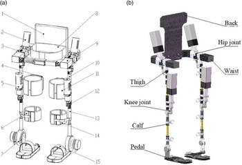
The developed lower limb exoskeleton is shown in Fig. 1. The exoskeleton robot designed in this paper mainly considers the motion in the sagittal plane. For each leg, it has one active degree of freedom (DoF) for the hip joint and knee joint, respectively, and one passive DoF for the ankle joint. The ankle joint has a high structural complexity, and it has an important influence on human walking stability [Reference Maharaj30–Reference Sato32]. Most of existing exoskeleton robots are designed with passive DoF ankle joint, such as Rewalk robot [Reference Esquenazi, Talaty and Packel4] and Mina exoskeleton robot [Reference Mummolo, Peng, Agarwal, Griffin, Neuhaus and Kim5]. On the one hand, it is to reduce the design difficulty and cost of the exoskeleton robot; on the other hand, the study found that when the ankle joint motion is disturbed by external interference, the walking stability of human body will be greatly reduced [Reference Sato32]. Hence, this study makes full use of the free movable property of the ankle joint to improve the walking stability.
(a) Overall structure diagram (1) back support; (2) actuators of hip joint; (3) hip joint component; (4) brace of thigh; (5) actuators of knee joint; (6) brace of calf; (7) ankle joint component; (8) flexible belt of waist; (9) waist component; (10) thigh component; (11) flexible belt of thigh; (12) knee joint component; (13) calf component; (14) flexible belt of calf; (15) pedal; (b). Exoskeleton mechanical diagram.

2.2 Dynamic modeling
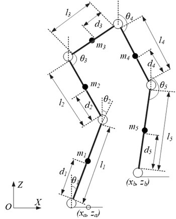
Lower limb exoskeleton robots are nonlinear, strongly coupled and multiple DoFs. In order to facilitate the completion of the center of gravity calculation and spatial state description, the structure needs to be appropriately simplified. The human reference coordinate system was established based on the human anatomical posture. The exoskeleton robot was simplified to a five-link model, just as shown in Fig. 2. The white circle is the joint and the black solid circle is the CoM of the linkage.
Five-link model.

The lower limb exoskeleton robot positional state is represented by a Cartesian coordinate system and generalized coordinates. The robot is supposed to walk in the sagittal XZ plane, and the ankle joint coordinates of the support leg and swing leg are (x a , z a ) and (x b , z b ), respectively. (x ci , z ci ) is the CoM coordinate of the linkage i, i = 1, 2,…, 5. l i is the length of each linkage of the lower limb; d i is the distance from the CoM of each linkage to the joint. m i is the sum of the mass of linkage i and its corresponding human lower limb. θ 1 , θ 2 ,…, θ 5 are the angles between each linkage and its vertical direction, and clockwise direction is positive. M 1 , M 2 ,…, M 5 are the joint torques of each linkage.
According to the geometric relationship in Fig. 2, the CoM coordinates of each rod are
 \begin{equation} \left\{\begin{array}{l} x_{ci}=\sum _{j=1}^{i-1}\left(s_{j}l_{j}\sin \theta _{j}\right)+d_{i}\sin \theta _{i}+x_{a}\\[8pt] z_{ci}=\sum _{j=1}^{i-1}\left(s_{j}l_{j}\cos \theta _{j}\right)+d_{i}\cos \theta _{i}+z_{a} \end{array}\right. \end{equation}
where i = 3, s j = 0; i = 1, 2, 4, 5, s j = 1.
Differentiating Eq. (1) with respect to time t, the velocity of each linkage CoM is obtained:
 \begin{equation} \left\{\begin{array}{l} \dot{x}_{ci}=\sum _{j=1}^{i-1}\left(s_{j}l_{j}\cos \theta _{j}\right)+d_{i}\dot{\theta }_{i}\cos \theta _{i}\\[8pt] \dot{z}_{ci}=\sum _{j=1}^{i-1}\left(-s_{j}l_{j}\sin \theta _{j}\right)-d_{i}\dot{\theta }_{i}\sin \theta _{i} \end{array}\right. \end{equation}
The total potential energy E p of the lower limb exoskeleton robot system is
 \begin{equation} E_{p}=\sum _{i=1}^{5}m_{i}gz_{ci}=\sum _{i=1}^{5}\left\{m_{i}g\left[\sum _{j=1}^{i-1}\left(s_{j}l_{j}\cos \theta _{j}\right)+d_{i}\cos \theta _{i}+z_{a}\right]\right\} \end{equation}
The total kinetic energy E k of the system is
 \begin{equation} \begin{array}{l} E_{k}=\sum _{i=1}^{5}\left\{\dfrac{1}{2}\left[m_{i}\left({\dot{x}^{2}}_{ci}+{\dot{z}^{2}}_{ci}\right)+I_{i}{\dot{\theta }^{2}}_{i}\right]\right\}=\sum _{i=1}^{5}\left\{\dfrac{1}{2}m_{i}\left[\sum _{j=1}^{i-1}\left(s_{j}l_{j}\cos \theta _{j}\right)+d_{i}\dot{\theta }_{i}\cos \theta _{i}\right]^{2}\right\}+\\[14pt] \sum _{i=1}^{5}\left\{\dfrac{1}{2}m_{i}\left[\sum _{j=1}^{i-1}\left(-s_{j}l_{j}\sin \theta _{j}\right)-d_{i}\dot{\theta }_{i}\sin \theta _{i}\right]^{2}\right\}+\sum _{i=1}^{5}\left\{\dfrac{1}{2}m_{i}{d^{2}}_{i}{\dot{\theta }^{2}}_{i}\sum _{j=1}^{i-1}\left[s_{j}l_{j}\dot{\theta }_{j}\cos \left(\theta _{i}-\theta _{j}\right)\right]\right\} \end{array} \end{equation}
where I i is the rotational inertia of the linkage i with respect to the CoM.
Substituting Eqs. (3) and (4) into the Lagrangian equation of the dynamical state of the lower limb exoskeleton robot system, the joint torque M i acting on joint i during robot walking is obtained from Eq. (5).
 \begin{equation} M_{i}=\frac{d}{d_{t}}\frac{\partial E_{k}}{\partial \dot{\theta }_{i}}-\frac{\partial E_{k}}{\partial \theta _{i}}+\frac{\partial E_{p}}{\partial \theta _{i}},\quad i = 1,2,\ldots,5 \end{equation}
3. Gait multi-objectives function design
In order to achieve stable walking of the lower limb exoskeleton robot, this paper abstracted the problem as a multi-objectives function optimization problem and constructed the multi-objectives function with the gait ZMP stability margin and the drive energy consumption per step. Since the hip joint is the closest joint to the human CoM, the change of the hip joint motion trajectory can be regarded as the change of the human CoM position, so the hip joint has a great influence on the ZMP trajectory and the gait stability of the exoskeleton robot. Assuming that the wearer’s hip joint is positioned midway between the two legs during walking, the constraint along the X-axis during a single step cycle is
 \begin{equation} \left\{\begin{array}{l} x_{hip}\left(0\right)=-S\\[5pt] x_{hip}\left(T\right)=S\\[5pt] \dot{x}_{hip}\left(t\right)\geq 0,t\in \left[0,T\right]\\[5pt] x_{l}\lt x_{zmp}\lt x_{r} \end{array}\right. \end{equation}
where x
hip
is the trajectory of the hip joint along the X-axis, and
 $\dot{x}_{hip}\left(\right)$
is the velocity of hip joint. T is the gait cycle, S is the step length and x
zmp
is the component of ZMP on the X-axis. x
l
and x
r
are the left and right boundaries of the support polygon, respectively.
And a fifth-order polynomial is used to represent the motion trajectory of the hip joint:
 \begin{equation} x_{hip}=-S+at+bt^{2}+\frac{1}{2}\rho _{1}t^{3}+\rho _{2}t^{4}+\frac{1}{2}\rho _{3}t^{5} \end{equation}
where ρ
1
, ρ
2
, ρ
3
are constant,
 $a=\frac{2S}{T}+\frac{1}{2}\rho _{1}T^{2}+\rho _{2}T^{3}+2\rho _{3}T^{4}, b=\frac{1}{2}\left(-2\rho _{1}T-4\rho _{2}T^{2}-5\rho _{3}T^{3}\right)$
.
3.1. Stability criteria
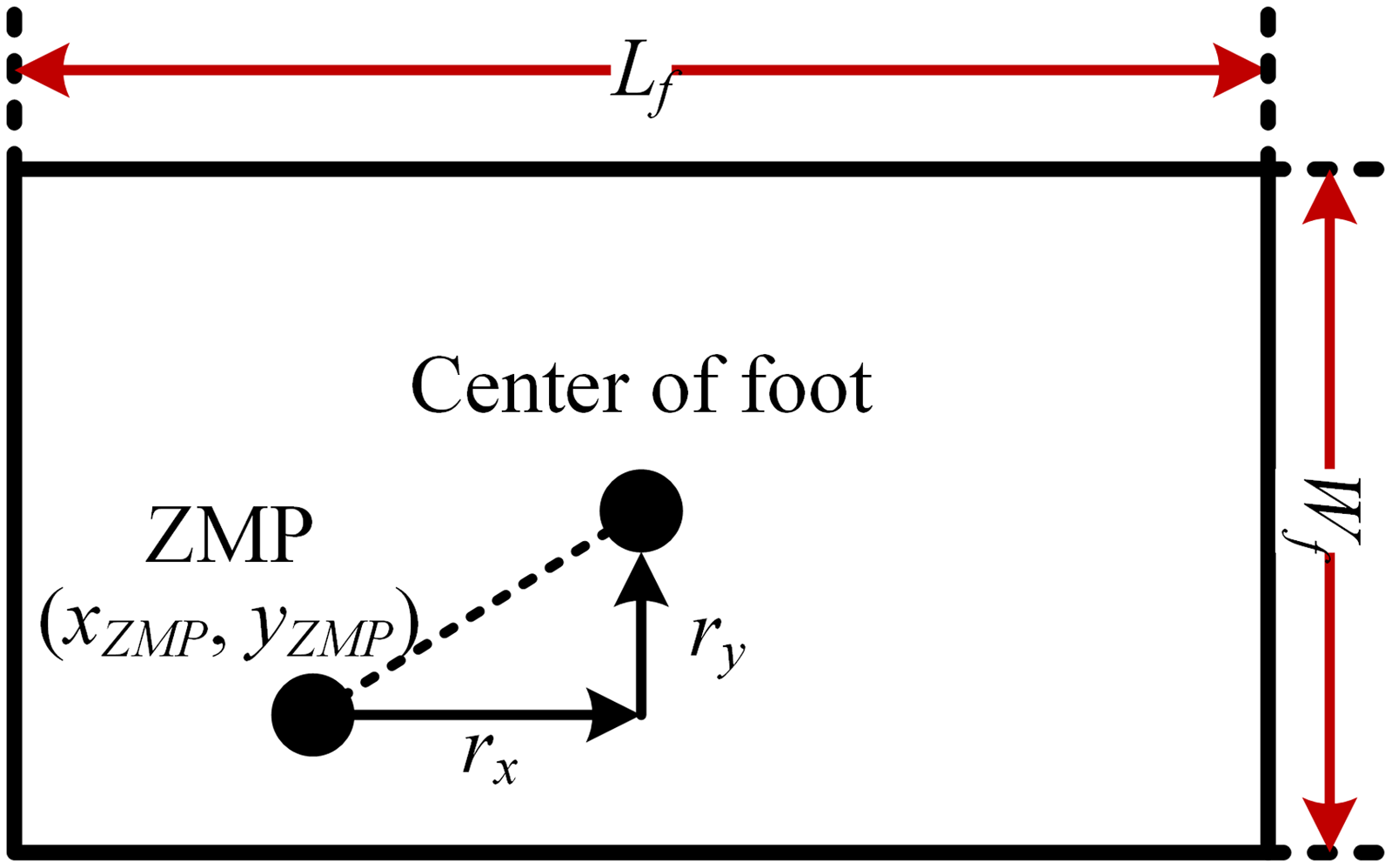
In order to comprehensively measure the degree of stability during robot motion, the ZMP stability margin J z was used to characterize the degree of stability in the horizontal direction, and the expression is shown in Eq. (8).
 \begin{equation} J_{z}=a\sum _{i=1}^{n}r_{x}\left(i\right)+b\sum _{i=1}^{n}r_{y}\left(i\right) \end{equation}
where
 $r_{x}\left(i\right), r_{y}\left(i\right)$
denote the distance from the ZMP point to the center of the foot in the x-axis and y-axis, respectively. n is the total number of the rod of exoskeleton robot. a and b are the weighting coefficients in the X-axis and Y-axis, respectively, and
 $a+b=1, \frac{a}{b}=\frac{L_{f}}{W_{f}}$
. L
f
denotes foot length, and W
f
denotes foot width, just as shown in Fig. 3.
ZMP stability margin diagram.

In the absence of external disturbance, exoskeleton robots mainly rely on the frictional torque to offset the influence of the deflection torque and maintain the balance of the torque in the vertical direction. Considering that the static friction torque is complicated to model and difficult to obtain accurately, the square of the deflection torque is used to characterize the stability in the equilibrium direction.
 \begin{equation} J_{b}=\left\| M_{b}\right\| _{2}^{2} \end{equation}
where M b is the deflection torque.
The ZMP is an important criterion used to check the stability of the robot. According to the definition of ZMP, the ZMP criterion can only ensure that the horizontal component of the torque around ZMP is 0, but its vertical component is generally not 0. As the torso and body parts will generate the swaying torque around the support leg during the forward motion, when the swaying torque exceeds the maximum frictional torque on the ground, the robot will rotate around the support leg, and the deflection caused by the excessive swaying torque is more obvious, so it is necessary to consider the torque balance between horizontal and vertical directions in the gait planning process. The M b is defined as:
 \begin{equation} M_{b}=\sum _{i=1}^{n}m_{i}\ddot{y}_{i}\left(x_{i}-x_{zmp}\right)-\sum _{i=1}^{n}m_{i}\ddot{x}_{i}\left(y_{i}-y_{zmp}\right) \end{equation}
 \begin{equation} x_{zmp}=\frac{\sum _{i}m_{i}\left(\ddot{z}_{i}+G_{\mathrm{g}}\right)x_{i}-\sum _{i}m_{i}\ddot{x}_{i}z_{i}}{\sum _{i}m_{i}\left(\ddot{z}_{i}+G_{\mathrm{g}}\right)} \end{equation}
 \begin{equation} y_{zmp}=\frac{\sum _{i}m_{i}\left(\ddot{z}_{i}+G_{g}\right)y_{i}-\sum _{i}m_{i}\ddot{y}_{i}z_{i}}{\sum _{i}m_{i}\left(\ddot{z}_{i}+G_{g}\right)} \end{equation}
where (x i , y i , z i ) is the coordinates of the CoM position of the i-th linkage, m i is the mass of the i-th linkage, n is the total number of links in the robot model and (x zmp , y zmp ) denotes the coordinates position of the ZMP.
3.2. Power consumption analysis
In terms of energy consumption, the minimum input energy of the driving joint is taken as the goal for the optimal solution of gait parameters. The average power method is an important measure of energy consumption analysis. Considering that the power of the machine is the product of motor drive torque and joint angular velocity, the average power P ave of the robot during a walking cycle can be characterized as:
 \begin{equation} P_{ave}=\frac{1}{T}\sum _{i=1}^{5}\int _{0}^{T}\left| M_{i}\left(t\right)\cdot \dot{\theta }_{i}\left(t\right)\right| dt \end{equation}
where M
i
(t) is the torque,
 $\dot{\theta }_{i}\left(t\right)$
is the joint velocity, and T is the gait cycle.
In the process of robot motion, the exoskeleton robot may be affected by external disturbances and its own structural deformation, resulting in the instantaneous power approaching infinity, but the average power at this time may be very small. The instantaneous power peak will reduce the stability of the entire system. In response to this situation, this paper introduces the root mean square deviation of the instantaneous power, which could accurately reflect the discrete degree between instantaneous power and average power.
 \begin{equation} P_{i}=\sum _{i=1}^{5}\left| M_{i}\left(t\right)\cdot \dot{\theta }_{i}\left(t\right)\right| \end{equation}
 \begin{equation} \sigma =\sqrt{\frac{1}{\left(T\right)}\int _{0}^{T}\left(P_{i}-P_{ave}\right)^{2}dt} \end{equation}
where P i is the instantaneous power. σ is root mean square deviation of instantaneous power.
3.3. The multi-objectives function design
We constructed the overall multi-objectives function
 $F\!\left(\mathbf{x}\right)$
for optimizing the exoskeleton robot system.
 \begin{equation} F\!\left(\mathbf{x}\right)=\alpha J_{z}+\beta J_{b}+\mu \left(P_{ave}+\sigma \right) F\!\left(\mathbf{x}\right)=\alpha J_{z}+\beta J_{b}+\mu \left(P_{ave}+\sigma \right) \end{equation}
where x is the vector, and
 $\mathbf{x}=\left[S,\rho _{1},\rho _{2},\rho _{3},\theta _{2},\theta _{3},\theta _{4},\theta _{5}\right]$
. α, β, μ∈ [0,1], the value is set according to the proportion of gait ZMP stability margin and driving energy consumption. The smaller the
 $F\!\left(\mathbf{x}\right)$
, the more stable and smooth the robot gait trajectory. In this study, the ideal gait could be obtained through optimizing the gait parameters. Therefore, multi-objectives function
 $F\!\left(\mathbf{x}\right)$
can be expressed as the optimized object function GoalF with gait parameters, and its expression is
 \begin{equation} \textit{GoalF}=\min \left[F\!\left(\mathbf{x}\right)\right] \end{equation}
4. Parameter optimization based on BSO-EOLLFF algorithm
4.1. Overview of BSO-EOLLFF algorithm
Based on the beetle antennae search algorithm and particle swarm optimization (PSO) algorithm, the BSO algorithm was designed [Reference Zhang and Zhang21, Reference Jiang and Li22]. The BSO algorithm has the characteristics of fast solving speed and high accuracy and has been successfully applied in the fields of signal positioning [Reference Liu, Qian and Jia23] and data classification [Reference Wu, Ma, Xu, Li and Chen24]. However, the BSO algorithm is easy to fall into the local optimum when searching in a high-dimensional space. In this regard, this paper introduced the EOL strategy, the LFF strategy and the dynamic mutation strategy to improve the optimization performance. In this study, we used EOL to initialize the population to promote a uniform distribution of initial population information and improve search efficiency. In addition, the LFF strategy enables the individuals to learn both their own and group experiences, allowing each individual to move purposefully and instructively and improving the convergence performance of the algorithm. Finally, a dynamic mutation strategy was introduced to increase the population diversity at the end of the iteration and prevent the algorithm from falling into the local optimum.
4.2. Population initialization based on EOL strategy
Tizhoosh introduced the concept of opposition-based learning in 2005 and showed that the inverse solution has a nearly 50% higher probability of being close to the global optimum than the current solution [Reference Tizhoosh25]. The main idea was that by generating reverse individuals in the area where the current individual was located and by competing for the reverse individuals with the current individuals, the best individuals will enter the next generation.
Definition 1. (Inverse solution): Let there exists a real number x
o
on the interval [e, u], then the inverse of x is defined as
 $x'_{\!\!o}=e+u-x_{o}$
. Based on this, it is assumed that there exists a certain n-dimensional solution point on the R-domain
 $p=\left(x_{o1},x_{o2},\cdots,x_{on}\right)$
, and
 $x_{oi}\in \left[e_{i},u_{i}\right]$
. The
 $p'=\left(x'_{\!\!o1},x'_{\!\!o2},\cdots,x'_{\!\!on}\right)$
is defined as the inverse solution of p, where
 $x'_{\!\!oi}=\lambda *\left(e_{i}+u_{i}\right)-x_{oi}$
, λ is a random number uniformly distributed in the interval [0,1], also known as the generalization factor.
Definition 2. (Optimization based on inverse solution). The problem to be optimized was a multi-objectives optimization problem, and if there exists a current solution X and its inverse solution is X′ , the following update mechanism is applied to X and X′ : (1) If X<X′ , keep the current solution X; (2) If X′ <X, replace X′ with X; (3) If X and X′ are not dominated by each other, then choose one of them at random.
Non-dominated solutions in multi-objectives optimization problems are generally considered elite individuals, usually containing more helpful information to guide the population to converge to the global optimum. The introduction of the inverse solution could expand the search area of the algorithm. Still, the search domain should be enhanced for those individuals in which original solution fitness value is greater than the inverse solution fitness value. For individuals whose original solution fitness value is smaller than the inverse solution fitness value, the value of searching the reverse area for them is higher than the value of developing their domain. Therefore, this paper took the individual whose original solution fitness value is smaller than the inverse solution fitness value as the research object and found its inverse solution, which could expand the search area and effectively avoid the time waste. If the final algorithm could converge globally, the search area formed by the elite individuals would converge to the search area formed by the global optimal solution set. Therefore, strengthening the search of the spatial neighborhood where the privileged individuals were located will increase the algorithm’s convergence speed and improve the algorithm’s global convergence ability.
Definition 3. (Elite inverse solution). Let the inverse solution of an elite individual
 $X_{best}=\left(x_{o1},x_{o2},\cdots,x_{on}\right)$
in a population p be
 $X'_{\!\!best}=\left(x'_{\!\!o1},x'_{\!\!o2},\cdots,x'_{\!\!on}\right)$
in an n-dimensional search space, and the elite inverse solution could be defined as
 $x'_{\!\!oi}=\lambda *\left(de_{i}+du_{i}\right)-x_{oi}$
.
 $\left[de_{i},du_{i}\right]$
is the dynamic boundary of the population P in the i-th dimensional search space and could be calculated according to (18).
 \begin{equation} de_{i}=\min _{1\leq j\leq \left| P\right| }\left(x_{oi}\right), du_{i}=\max _{1\leq j\leq \left| P\right| }\left(x_{oi}\right) \end{equation}
where
 $\left| P\right|$
is the size of the current group.
The dynamic boundary of the search space was used instead of the fixed boundary to preserve the search experience so that the generated inverse solutions could be located in the gradually shrinking search space and promote the faster convergence of the algorithm. Since the elite inverse solution may also jump out of the boundary
 $\left[e_{i},u_{i}\right]$
and become non-feasible, the method in the literature [Reference Zhou, Wu and Wang26] was used here to reset the transgressed values, as shown in (19):
 \begin{equation} x'_{\!\!oi}=rand\left(e_{i},u_{i}\right), e_{i}\lt x'_{\!\!oi} \;\;\textrm{or}\;\; u_{i}\gt x'_{\!\!oi} \end{equation}
By forming the elite inverse solution, the detection of elite individuals’ neighborhoods can be enhanced. The BSO algorithm performs reverse learning for the elite individuals of each iteration to generate the reverse population of elite individuals and participate in the evolutionary competition.
4.3. LFF strategy
In the standard BSO algorithm, the search range of beetle individuals was limited, and it is difficult to transfer the search position from the global optimal to the local optimal. Although the group search could expand the search range, there is no information exchange and feedback between the individuals, which will affect the convergence accuracy of the algorithm. The individuals in the group need to continuously learn the experience of the historical information, which plays a decisive role in the improvement of the algorithm’s convergence speed. Therefore, the LFF strategy was introduced. LFF strategy was proposed by Levy in the 1930s, and Mandelbrotb described it in detail [Reference Jiadong, Xinqian, Qian, Haitao and Xiaolin27]. The strategy obeys the Levy distribution. LFF strategy could increase the diversity of the population, expand the search range and prevent the algorithm from falling into the local optimum. The Levy distribution satisfies:
The calculation formula of the step length s is
 \begin{equation} s=\frac{\psi }{\left| \nu \right| ^{\frac{1}{\varphi }}} \end{equation}
where
 $\psi$
and ν obey normal distribution,
 $\mu,v\sim N\left(0,\sigma ^{2}\right)\mu \sim N\left(0,\sigma _{\mu }^{2}\right), \nu \sim N\left(0,\sigma _{\nu }^{2}\right)$
.
 $\varphi$
is constant
 \begin{equation} \sigma _{\psi }=\left[\frac{\Gamma \left(1+\varphi \right)\ast \sin \dfrac{\pi \varphi }{2}}{\Gamma \left(\dfrac{1+\varphi }{2}\right)\ast \varphi \ast 2^{\frac{\varphi -1}{2}}}\right]^{\frac{1}{\varphi }} \end{equation}
where Γ() is the standard gamma distribution.
The update rule of beetle direction is
 \begin{equation} d\!\left(t+1\right)=\omega \ast d\!\left(t\right)+C_{1}\ast Levy\!\left(\theta \right)\ast \left(\textit{gbest}\left(t\right)-X\!\left(t\right)\right)+C_{2}\ast Levy\!\left(\theta \right)\ast \left(\textit{zbest}\!\left(t\right)-X\!\left(t\right)\right) \end{equation}
The update rule of beetle position is
 \begin{equation} X\!\left(t+1\right)=X\!\left(t\right)+k_{1}*s*d\!\left(t\right)*sign\!\left(f\!\left(X_{r}\!\left(t\right)\right)-f\!\left(X_{l}\!\left(t\right)\right)\right)+k_{2}d\!\left(t\right) \end{equation}
where d(t) represents the movement direction of the t-th generation. X(t) represents the beetle position of the t-th generation. gbest() represents the individual extreme value of the t-th generation beetle. zbest() represents the global extreme value. ω is the inertia weight, and C 1 and C 2 are the learning factors. Levy(θ) is a Levy random number. f(x r (t)) and f(x l (t)) are the fitness function value of the right whisker and left whisker of the t-th generation longhorn beetle. k 1 and k 2 are the scale factor. sign() is a sign function.
4.4. Dynamic mutation strategy
In the later stage of the iteration, the population diversity of the BSO algorithm will become lower, which will reduce the search ability of the algorithm. To avoid premature phenomena, a dynamic mutation strategy was introduced to increase the diversity of the population and improve convergence accuracy. At present, related scholars have proposed a variety of mutation algorithms, and the typical ones are Gaussian mutation [Reference Ni, Ling, He and Hai28] and Cauchy mutation [Reference Rudolph29]. Compared with the Gaussian mutation, the Cauchy mutation could generate a more extensive range of random numbers so that the algorithm has a greater chance to jump out of the local optimum. Meanwhile, when the peak value is small, the Cauchy mutation only takes less time to search nearby areas. The Cauchy mutation was selected for the second optimization of the population, and the mutation operation was performed on X(t):
 \begin{equation} X^{*}\!\left(t\right)=X\!\left(t\right)+\zeta *C\!\left(0,1\right) \end{equation}
 \begin{equation} \zeta =e^{-\gamma \frac{t}{H}} \end{equation}
where ζ is the weight of mutation, which will decrease with increasing iteration. H is the maximum number of iteration. γ is constant. C(0,1) is a random number generated by Cauchy operator.
4.5. The basic steps and verification of BSO-EOLLFF algorithm
Because of a large number of parameters to be optimized for the objective function in this paper, the process of gradually approximating the optimal value is complicated, the accuracy of the optimized solution is not high, and the convergence speed is relatively slow. During the search process of the traditional PSO algorithm, the position of each particle is approached toward the global optimal position in a decreasing sine wave manner. During this process, a particle converges to the currently found global optimum position, and the other particles will quickly converge to this local optimum solution. If this optimal position is only a local optimal point, then most of the particles are confined by this local optimal solution. To overcome the shortcomings of traditional algorithms, the BSO-EOLLFF optimization algorithm is proposed in this paper. According to the gait parameters to be optimized, the population individuals are selected as
 $x_{p}=\left[S,\rho _{1},\rho _{2},\rho _{3},\theta _{2},\theta _{3},\theta _{4},\theta _{5}\right]$
in the improved algorithm. Since the ankle joint has a passive DoF, θ
1
is not used as an optimization parameter. According to Eq. (16), the fitness value corresponding to the multi-objectives function
 $F\!\left(\mathbf{x}\right)$
at each point x
p
was calculated.
4.5.1. The steps of BSO-EOLLFF algorithm
The specific steps of the BSO-EOLLFF algorithm are:
-
1. Initialize the algorithm parameters: the beetle scale, iterative step length and the maximum number of iterations. Use the EOL strategy to initialize the beetle population and initialize the direction.
-
2. Calculate the corresponding fitness function value of the beetle and determine the individual extreme value and the global extreme value according to the fitness function value.
-
3. Use (22) and (23) to update the direction and position of the beetle individuals and perform cross-border processing of beetle populations.
-
4. Use (24) to perform mutation operation on population.
-
5. Determine whether the algorithm meets the iteration termination condition. If it is satisfied, output the optimal global solution and its corresponding position, otherwise return to step 2.
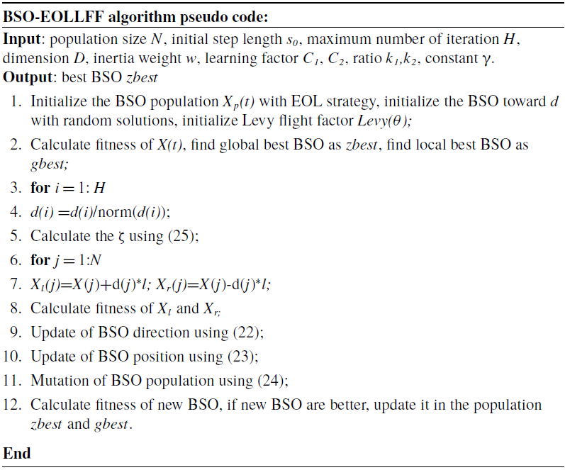
The pseudo code of BSO-EOLLFF algorithm is shown in Table I.
Psedo code of BSO-EOLLFF algorithm.

Parameters setting of the two algorithms.

4.5.2. Performance analysis of BSO-EOLLFF algorithm
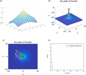
In order to verify the performance of the BSO-EOLLFF algorithm, the Rastrigin function
 $z=-20e^{-0.2\sqrt{0.5\left(x^{2}+y^{2}\right)}}-e^{0.5\cos \left(2\pi x\right)+\cos \left(2\pi y\right)}+20+2.72$
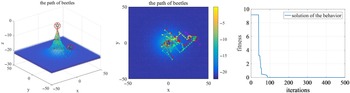
with lots of local solutions was selected to perform function optimization and convergence test. The parameter setting of the two algorithms is shown in Table II. The test results are shown in Fig. 4. The BSO-EOLLFF algorithm could accurately search for the optimal solution and would not fall into the local optimization. The algorithm’s search time is 1.35 s. To verify the superiority of the BSO-EOLLFF algorithm, the PSO algorithm was used to perform parameter search for the same test function, and the experimental results are shown in Fig. 5. The experimental results showed that although the PSO algorithm can eventually obtain the global optimal solution as well, there are four local optimal solutions in the process of finding the optimal solution, and the time to find the optimal solution is 5.73 s, which is significantly slower than the algorithm proposed in this study. The experimental results showed that the algorithm proposed in this study has a significant effect enhancement for the regular test function.
Optimization results of BSO-EOLLFF algorithm for the test functions. (a) Test function diagram, (b) optimal trace of each test function, (c) the contour map of the search path and (d) the convergence curves.

Optimization results of PSO algorithm on the test functions. From left to right: optimal trace of each test function, the contour map of the search path, and the convergence curves.

5. Simulation experiment analysis
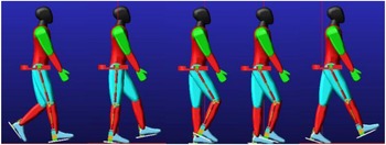
SolidWorks, ADAMS and MATLAB software were used to conduct a joint comparison test to verify the performance of the optimization algorithm proposed in this paper. The 3D model of the lower limb exoskeleton robot built in SolidWorks software was imported into ADAMS software for gait characteristics analysis, and the parameter characteristics were passed to MATLAB software for gait optimization through the relevant interface. MATLAB software imported the optimized multi-objectives gait information into ADAMS software again through the control module to analyze the gait stability. The robot virtual prototype and simulation environment are shown in Fig. 6.
The human-exoskeleton simulation process diagram.

5.1. Parameter setting
The mechanism parameters of the lower limb exoskeleton robot are set as: m
1
= 2 kg, m
2
= 2.5 kg, L
1
= 0.37 m, L
2
= 0.4 m. The number of beetles n is 50, the maximum number of iterations H is 1000, inertia weight w is 0.8, individual learning factor C
1
is 1.8, and global learning factor C
2
is 1.4. The ratio k
1
and k
2
are 0.4 and 0.6, respectively. The initial weight of mutation is 0.7. The initial step length s
0
is 1. The gait cycle T is 1 s. The constant γ and
 $\varphi$
are 10 and 1.5, respectively. In the iterative process, the condition for the iteration termination is that the error of parameter optimization is less than 0.1. In order to avoid the chance of experimental results, we conducted five simulation experiments and took the average of the experimental results for analysis.
5.2. Convergence analysis
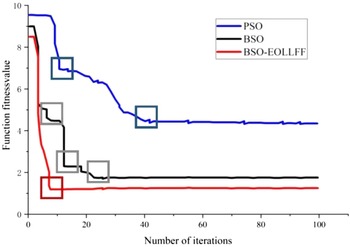
In order to avoid the BSO algorithm from falling into the local optimum, the EOL algorithm with global search capability, the LFF algorithm with local search capability and the dynamic mutation strategy with high population diversity were introduced to improve the optimization performance. To verify the convergence of the BSO-EOLLFF algorithm, the convergence curves of each algorithm were compared with the PSO algorithm and BSO algorithm, respectively, as shown in Fig. 7.
Convergence curve of each algorithm.

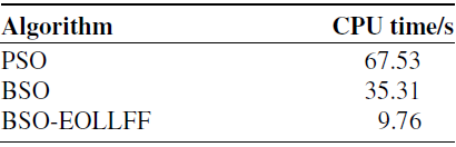
It can be seen from Fig. 7 that the traditional PSO algorithm stops searching after 40 iterations and falls into the local optimum due to its weak global search ability [Reference Zhang and Zhang21]. When the BSO algorithm iterates 23 times, the function fitness value tends to be stable. However, it has three local optimal solutions (gray square), which will affect the convergence. Although it is lower than the global optimal value found by the PSO algorithm, the convergence speed is slower. The BSO-EOLLFF algorithm searches for the optimal solution when iterated 8 times. The BSO-EOLLFF could find the only global optimal value, which is the lowest. And the averaged convergence time is shown in Table III. The time consumption of the algorithm is 9.76 s, which is significantly faster than the other two algorithms. After the comparative analysis of the search time, the efficiency of the BSO-EOLLFF algorithm was not weakened after the addition of the EOL algorithm and LFF algorithm, which indicates that the fit and conversion between the algorithms are good. The strategy proposed in this paper increases the diversity of the population, which speeds up the algorithm search speed and further improves the optimization accuracy.
5.3. Stability analysis
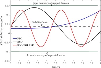
To further verify the stability of the BSO-EOLLFF algorithm proposed in this paper, the gait ZMP stability margin and joint driving energy consumption of the lower limb exoskeleton robot optimized by the three algorithms were compared and analyzed. The exoskeleton robot’s ZMP stability margin curves were optimized using the PSO algorithm, the BSO algorithm and the BSO-EOLLFF algorithm, as shown in Fig. 8.
It can be seen from Fig. 8, in one gait cycle, after the optimization of the PSO algorithm, the gait ZMP of the robot only passes through the stable center-line once. The trajectory of the center of gravity of the robot deviates from the bipedal support area, and the human body is prone to fall when walking. After optimizing by the BSO algorithm, the gait ZMP trajectory is close to the boundary. The minimum distance between the gait ZMP trajectory and the upper boundary is 0.0063 m. There are two times passing the stability center-line. The robot’s center of gravity trajectory is roughly distributed in the middle of the bipedal support domain, which has an ideal stability margin. The ZMP optimized by the BSO-EOLLFF algorithm has better performance. The closest gait ZMP point to the boundary line of the support domain is 0.1272m. At this time, the minimum distance between the two is 0.0228 m. The gait ZMP trajectory is uniformly in the middle of the support domain, which can realize stable walking.
5.4. Energy consumption analysis
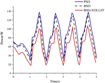
As can be seen from Fig. 9, the drive energy consumption of the robot increases and then decreases with each walking step, which is because the magnitude of the torque required by the joints in the oscillation process is mainly determined by the work done by gravity. To thoroughly verify the effectiveness of the proposed optimization algorithm, the minimum, maximum and average values of the drive energy consumption of the robot in 100 walking cycles optimized by the three algorithms were selected for comparison, and the algorithm energy consumption is shown in Table IV.
The averaged convergence time.

ZMP stability margin curve after algorithm optimization.

Gait drive energy consumption curve.

6. Human-machine experiments and results analysis
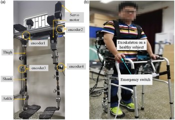
Human-machine experiments are conducted to demonstrate the functionality of the proposed control method. The exoskeleton robot platform is shown in Fig. 10. The range of motion of the human hip and knee joints is −40°−145° and 0°−145°, respectively. The joint motion range of the exoskeleton is 20° flexion and 40° extension for the hip joint, and 80° flexion and 0° extension for the knee joints. According to refs. [Reference Mihcin33, Reference Mihcin, Ciklacandir, Kocak and Tosun34], the designed exoskeleton robot in this paper conforms to the standardization (ISO)13485. The actuator of the joint is independent and the motion speed is designed with a uniform speed of 0.3 m/s. The control system consists of the data processor Raspberry Pi and the motion controller STM32F103. Raspberry Pi is used to process data collected from angle sensors (AD36/1217AF. ORBVB, Hengstler, Germany). The communication mode between the data processor and motion controller is parallel port communication. The motion controller controls the motors through the controller area network fieldbus. Encoder 1 and encoder 2 are used to acquire the movement data of the hip joint, and encoder 3 and 4 together record the knee joint angle. For safety reasons, if the angle of the exoskeleton is greater than the allowable value, the exoskeleton will be forced to stop moving by software. In addition, the subject could cut off the power through the emergency switch button.
The main goal of this paper is to make the gait generated by the exoskeleton more efficient and stable through multi-objectives optimization. Therefore, the joint motion trajectory and ZMP trajectory(
 $x_{ZMP}^{ref}\left(\right)$
and
 $y_{ZMP}^{ref}\left(\right)$
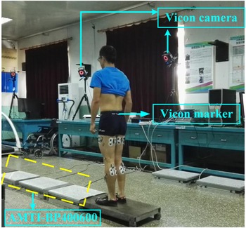
) of the human body need to be obtained and used as the reference trajectory. A healthy subject with the age of 25, the weight of 68 kg and the height of 170 cm is recruited for the experiment, just as shown in Fig 11. Before the gait experiment, the subject was given a detailed explanation of the test content and signed a consent form for voluntary participation in the experiment. The subject had no surgery, no history of lower extremity trauma, no balance problems or neural muscular disorders within the past six months. A written consent is obtained from the subject. The test environment was a linear walkway of 5 m in length and 1 m in width, just as shown in Fig 11. The kinematic parameters were acquired by VICON acquisition system (Oxford Metrics Ltd, Oxford, UK). Ground reaction force was recorded by two AMTI force plates (AMTI Corp, Newton, USA). The data acquisition frequency is 1200 Hz. The VICON system and AMTI system are time-synchronized.
Energy consumption analysis.

(a) Prototype of the proposed exoskeleton robot and (b) Human-machine experiment.

Gait experiment diagram.

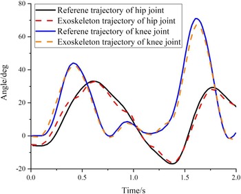
Comparative analysis of joint trajectories.

The figure for the joint position of the hip joint and the knee joint is shown in the Fig. 12. The agreement between the reference trajectory and the actual trajectory illustrates the effectiveness of the control method. In general, comparisons between a pair of kinematic or kinetic curves are performed by calculating the Pearson correlation coefficient (R), which quantifies the strength of the linear relationship between the two curves (i.e. similarity of their shapes) [Reference Iosa, Cereatti, Merlo, Campanini, Paolucci and Cappozzo35]. The results of R are shown in Table V. The experimental results show that the tracking performance of the BSO-EOLLFF controller designed in this paper is good, and the overall average error of hip joint position and knee joint position is 0.669 and 0.877 deg, respectively. And the biggest error generated during the whole exercise of hip joint position and knee joint position is 1.981 and 1.319 deg, respectively, which meets the training requirements of the lower limb rehabilitation robot.
 \begin{equation} R=\frac{\mathrm{cov}\!\left(X,Y\right)}{\sigma _{X}\sigma _{Y}} \end{equation}
 \begin{equation} \mathrm{cov}\!\left(X,Y\right)=E\left[X-E\!\left(X\right)\left(Y-E\!\left(Y\right)\right)\right] \end{equation}
 \begin{equation} \sigma _{X}=\sqrt{\frac{\sum _{i=1}^{n}\left(X-\overline{X}\right)^{2}}{n}} \end{equation}
where E(X) and E(Y) are the expected value of variable X and Y, respectively.
 $\overline{X}$
and
 $\sigma _{X}$
are the mean value and standard deviation of the sample X. In this paper, X and Y represent the reference trajectory and the actual trajectory, respectively.
We collected the energy consumption values for six gait cycles and take the average value to obtain the average power consumption for a gait cycle. The average power value of the BSO-EOLLFF algorithm for trajectory energy optimization is 65.8 W. Compared with the traditional PSO algorithm, the average power value was decreased by 30.5 W.
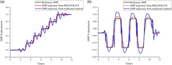
Figure 13 gives a comparison of the actual ZMP trajectories for the two sets of experiments. The magnitude of the ZMP tracking error in the X-direction and Y-direction is measured by E x and E y , respectively:
Analysis of reliability: Results of R.

Comparison analysis of ZMP trajectory. (a) X-direction; (b) Y-direction.

 \begin{equation} E_{x}=\int _{t_{0}}^{t_{f}}\left[x_{ZMP}^{ref}\left(t\right)-x_{ZMP}\left(t\right)\right]^{2}dt \end{equation}
 \begin{equation} E_{y}=\int _{t_{0}}^{t_{f}}\left[y_{ZMP}^{ref}\left(t\right)-y_{ZMP}\left(t\right)\right]^{2}dt \end{equation}
where
 $x_{ZMP}^{ref}\left(\right)$
and
 $y_{ZMP}^{ref}\left(\right)$
are the ZMP reference value in X-direction and Y-direction, respectively.
 $x_{ZMP}\left(\right)$
and
 $y_{ZMP}\left(\right)$
are the ZMP actual value in x-direction and y-direction, respectively. t
0
and t
f
are start time and end time of gait cycle, respectively.
Compared with the traditional method, Ex is reduced by 45.3%, and Ey is reduced by 52.7%. In Fig. 13, it is evident that the exoskeleton robot system can effectively eliminate the disturbance during the walking process. In the X-direction, the reference ZMP trajectory can be tracked better, and the oscillation phenomenon is not apparent. In the Y-direction, compared to the reference ZMP trajectory, the method proposed in this study produces a specific deviation with an overall average error of 0.035m, which is a significant progress compared to the traditional method.
7. Conclusion
A vital issue for exoskeleton robots is maintaining gait stability during walking to prevent the wearer from falling. By reducing the minimum distance between the ZMP and the center of the foot, increasing the number of intersections between the ZMP and the stability center-line and reducing the drive energy consumption, it can be judged that the stability margin of the ZMP after the parameter optimization of the BSO-EOLLFF algorithm has been improved considerably. The robot gait can achieve stable and smooth walking with less energy consumption, which fully demonstrates the effectiveness of the BSO-EOLLFF algorithm. The agreement between the reference trajectory and the actual trajectory illustrates that the applicability of the proposed algorithm in robot walking is better, and the rationality and reliability of planned walking are ensured. In the future, the exoskeleton will also consider additional movement modes, such as climbing steep hills and running. In each motion mode, dynamic stability and exoskeleton interference forces will be analyzed in detail, and adaptive control strategies adapted to each motion mode will be designed.
Ethical approval
Not applicable.
Consent to participate
Not applicable.
Consent to publish
The work described has not been submitted elsewhere for publication, in whole or in part, and all the authors listed have approved the manuscript that is enclosed.
Authors contributions
All authors have made substantial contribution. The first author Peng Zhang designed the experiment scheme, analyzed the experimental results and wrote the paper. Corresponding author Junxia Zhang and third author Ahmed Elsabbagh modified the paper.
Competing interests
Not applicable.
Funding
This work was supported in part by the Hundred Cities and Hundreds Parks Project-Key Nutrition and Health Technology and Intelligent Manufacturing (21ZYQCSY00050), Tianjin Science and Technology Plan Project (20JCYBJC01430) and China Scholarship Council.
Availability of data and materials
Not applicable.