

Many electoral reforms are intended to improve democratic representation by changing aggregate legislative outcomes. Advocates of electoral reforms often predict normative improvements in policy adoption or representation driven by expected changes in the composition of the legislature and changes in incumbent legislator behavior. Extolling the virtues of the Top Two primary, under which candidates from all parties compete with one another and the top two vote-getters advance to a runoff election, California Gov. Arnold Schwarzenegger argued that implementing this reform would “force [legislators] to appeal to a broader number of voters … It will free legislators from their ideological straight-jackets, so they can meet in the middle and get things done” (Myers Reference Myers2018). While Schwarzenegger focused on the changes in incumbent behavior that the Top Two primary would induce, this institutional change could also change the ideological composition of candidates who run for office and those who win elections.
How reforms affect the ideological positions of challengers who run for office is particularly important when incumbent legislators exhibit persistence in their behavior. Empirical evidence shows that incumbents do not fully change their voting behavior when the political context and electoral environment changes (Poole Reference Poole2007). If incumbents do not fully adapt to new electoral conditions, the full effect of electoral reforms on aggregate legislative outcomes will not occur until all incumbent legislators are replaced by new entrants.Footnote 1
An important literature in political science examines how reforms such as campaign finance regulations (La Raja and Schaffner Reference La Raja and Schaffner2015; Barber Reference Barber2016), changes to legislative compensation (Hall Reference Hall2019), and non-partisan redistricting commissions (Grainger Reference Grainger2010; McGhee and Shor Reference McGhee and Shor2017) affect partisan polarization in legislative bodies. We contribute to this literature by developing a simple theoretical framework to show that the magnitude of the effect sizes of these reforms depends upon whether an electoral reform is implemented or removed. Our framework reveals that implementing a moderation-inducing reform, such as unlimited PAC contributions, will produce an effect of a larger magnitude on polarization than repealing the same reform. The reason for this asymmetry is that incumbents experience lower reelection rates when a moderation-inducing reform is implemented relative to when it is removed. As a result, each party will experience greater turnover when the moderation-inducing reform is first implemented and less turnover when the moderation-inducing reform is removed. We then examine whether these novel empirical predictions hold in the context of campaign finance reforms in the states. The estimates are consistent with our theoretical predictions.
Our theoretical results are driven by two key assumptions. First, electoral reforms change the ideological positions of challengers, but incumbents cannot perfectly adjust their ideological location to be equivalent to their party's challengers. We refer to this assumption as incumbent policy persistence (Forand Reference Forand2014).Footnote 2 Second, we assume that the ideological proximity between a candidate and the pivotal citizen's ideal policy positively affects the probability that the citizen votes for the candidate. As we discuss below, there is compelling empirical evidence for both of these assumptions. Incorporating these stylized facts into a dynamic model of elections, we show that incumbent reelection rates increase when a moderation-inducing reform is removed and decrease when the reform is implemented. We then show that the magnitude of the change in partisan polarization, as measured by the distance between the average ideological position of right-party legislators and left-party legislators, is greater when the reform is implemented than when it is removed.
Our analysis helps clarify several important issues in the empirical literature on how electoral reforms affect legislative polarization. When studying the effects of electoral reforms on aggregate legislative behavior, it is necessary to distinguish between how the electoral reform affects the behavior of current legislators, the behavior of challengers, and the probability that the pre-reform incumbents are replaced by new entrants. The empirical literature does not always differentiate between these different components. For example, in Table 4.2 of La Raja and Schaffner (Reference La Raja and Schaffner2015), the authors estimate a regression of legislature-wide polarization on an indicator for whether there are limits on parties’ ability to raise funds. This analysis cannot distinguish between the effects of the campaign finance reform on the ideological location of incumbent legislators, challengers, and the probability that the pre-reform incumbents are reelected. In contrast, Barber (Reference Barber2016) estimates the effect of campaign finance regulations on the roll-call voting behavior of new entrants to the legislature.Footnote 3 This approach is justified by the assumption that roll-call voting is relatively stable over time so any treatment effect would be limited to new legislators. Our framework illustrates why this cohort analysis is important for estimating the long-run treatment effect.
Our framework can be used to analyze the entire dynamic path of a reform's effects on polarization. After many elections, none of the incumbents who were in office before the reform was implemented or removed will remain in office. As a result, the long-run effect of an electoral reform on legislature-wide polarization will be equal to the effect on challengers’ ideological locations. These dynamics are an important consideration when estimating the effects of electoral reforms. While the effects of an electoral reform on legislative polarization might appear to be small immediately after reform implementation, they can increase dramatically as more legislators are replaced with new entrants.
Finally, our analysis shows that there is an important and typically-ignored interaction between electoral reforms that directly affect legislative polarization and reforms that affect the probability that incumbents continue in office.Footnote 4 Term limits are the most clear-cut example. Term limits deterministically require legislators to exit from office after a fixed number of terms. As a result, new challengers, who are not constrained by incumbent policy persistence, will enter the legislature and the full effects of the electoral reform will manifest themselves more rapidly than in a state without term limits. As we show below, we find evidence consistent with this interaction in the context of unrestricted PAC contributions and term limits. More generally, any institutional change that influences the magnitude of the incumbency advantage or the private returns to officeholding will moderate the polarization effect through the effect on the probability that incumbents continue in office.
Justifying the assumptions
Before proceeding to the theoretical analysis, we justify and elaborate on the two key theoretical assumptions that drive the results. Our first assumption is that incumbents exhibit some degree of ideological policy persistence. Relative to challengers, it is more difficult for incumbents to change the ideological positions that they have adopted. There are a number of sources of ideological persistence among incumbents. First, legislators may have personal ideological convictions that they are not willing to change under normal circumstances. Second, even if there are changes in the electoral environment, voters may penalize politicians that change ideological positions. A central reason that incumbents may choose to persist in their ideological positions despite changing electoral circumstances is that voters negatively evaluate candidates who adjust their policy positions. In the context of US politics, Tomz and Van Houweling (Reference Tomz and Van Houweling2012) use experimental vignettes and DeBacker (Reference DeBacker2015) employs data from US Senate elections to show that voters penalize candidates who engage in ideological adjustment. As a result, it can be electorally costly for an incumbent to locate at a new ideological position. An incumbent will not change positions if the costs of adapting are larger than the benefits of adopting a new policy stance.Footnote 5
The ideological position of general election challengers, on the other hand, is more flexible than that of incumbents for at least two reasons. First, the average challenger has a less well-defined public record of policy positions than the average incumbent (Peskowitz Reference Peskowitz2019). Therefore, they can more easily change ideological positions to adapt to a new electoral environment after a reform is implemented or removed. Second, general election challenger candidates are typically selected among a large pool of potential challengers through a primary election process. An electoral reform may impact which challenger from the pool of potential challengers is ultimately successful in the primary, which will affect the ideological position of a general election challenger.
The empirical evidence on whether incumbent legislators in the United States change their ideology as measured by their roll-call voting behavior is ambiguous. While some scholars argue that members of Congress do not change their roll-call voting over time (Poole Reference Poole2007), others have found evidence of ideological adaptation to changing electoral circumstances (Stratmann Reference Stratmann2000; Kousser et al. Reference Kousser, Lewis and Masket2007; Kogan Reference Kogan2016). While we assume that incumbent policy positions are completely persistent in our discussion of the results below, the extreme version of this assumption is not necessary to derive our key results. As we show in the Online Appendix, in the more realistic case that incumbents have some ability to change their ideological positions but cannot perfectly adjust to the location of their party's challengers, then our main results still hold.
The other essential assumption is that increasing the ideological distance between a candidate and the pivotal voter decreases the probability that the candidate wins the election. We do not assume that ideological proximity is the only factor that affects voter utility. Our results still hold if citizens have preferences over candidates’ non-ideological valence characteristics or if voters choose between candidates probabilistically. There is compelling evidence to support this assumption.Footnote 6 Burden (Reference Burden2004) finds a positive association between the spatial proximity of House candidate to the voters and the candidate's electoral performance. At the state level where we perform our empirical application, Birkhead (Reference Birkhead2015) finds that in the average state legislature moderates electorally outperform extremist candidates. Hall (Reference Hall2015) uses a regression discontinuity design to show that when ideologically extreme US House candidates narrowly win a partisan primary over a moderate candidate, their party performs dramatically worse at the ballot box in the subsequent general election.
Electoral reforms, incumbent reelection rates, and polarization dynamics
We develop a simple decision theoretic framework to show how electoral reforms affect the dynamics of partisan polarization. The only optimizing agent in our framework is the voter who chooses between candidates on the basis of ideological proximity and a stochastic error term. We do not microfound the spatial locations of the incumbents and challengers and instead take these locations as exogenous parameters. Our framework analyzes electoral reforms in the context of a general election with a left party candidate facing off against a right party candidate.Footnote 7
We present the intuition behind our main theoretical results in a series of figures for a simple parametric example.Footnote 8 In the Online Appendix, we generalize these results to the setting where incumbents have asymmetric ideological positions.Footnote 9 We compare two states that both have the same level of initial partisan polarization, but differ in their electoral institutions. In one state, the moderation-inducing reform will be implemented, and in the other state, the reform will be removed. We assume that electoral reforms operate by shifting the location of the challenger. When a moderation-inducing reform is implemented, the challengers shift toward the pivotal voter by a factor of τ/2, while when a moderation-inducing reform is removed, the challengers shift away from the voter by the same τ/2 distance.
The assumption that challengers shift toward the pivotal voter in response to the implementation of a moderation-inducing reform is more straightforward to justify on the basis of candidate electoral considerations than the assumption that challengers shift away from the pivotal voter when a moderation-inducing reform is removed. However, there are settings where this assumption is more plausible. For example, if implementing a limit on PAC contributions increases the probability that extreme candidates will win primaries then we will observe more extreme general election candidates on average when the reform is removed. More importantly, our main results on the relative magnitudes of the effects of electoral reforms on aggregate polarization still hold if the challengers do not change their location when the moderation-inducing reform is removed. If we were to assume that challengers are located at the incumbents’ locations when the moderation-inducing reform is removed, there would be no effect of removing the moderation-inducing reform on incumbent reelection rates or aggregate polarization.
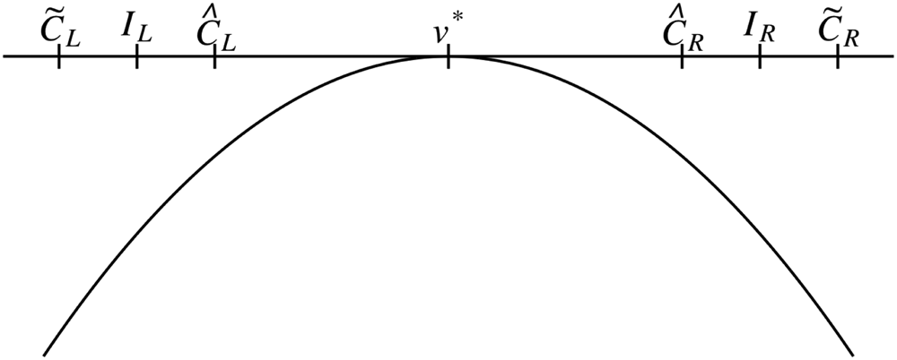
In Figure 1, we plot the deterministic spatial component of the voter's utility function for incumbents and challengers. Based on our assumption of incumbent policy persistence, the incumbent's ideological location remains the same regardless of the reform and is indicated by I L and I R for the left and right party incumbents, respectively. However, the challenger's ideological location is shifted by the institutional reform. When the reform is removed, the challengers are more ideologically extreme than the incumbents and the ideological position is denoted by $\widetilde {C}_L$ and $\widetilde {C}_R$
 . In contrast when the reform is implemented, the challengers are more moderate with positions $\hat {C}_L$
 and $\hat {C}_R$
 .
Voter's spatial utility.

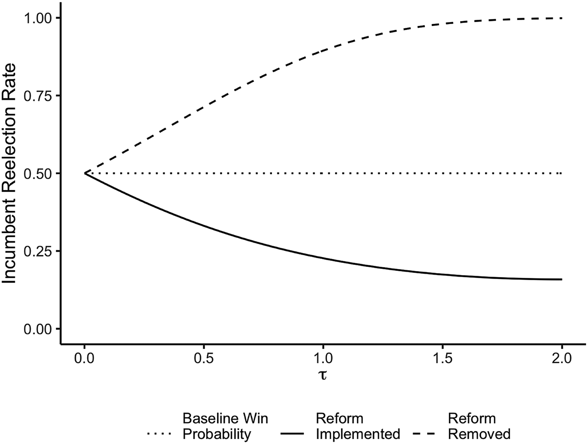
As an immediate consequence of our assumptions, the probability that the incumbent is reelected differs across the two states. In the state where the moderation-inducing reform is implemented, the reelection probability of the incumbent is reduced relative to the baseline while this probability increases when the reform is removed. In Figure 2, we plot the probability that an incumbent wins reelection as a function of the treatment effect magnitude under the alternative electoral reform scenarios. Figure 2 also reveals that the magnitude of the change in the reelection rates depends upon the strength of the ideological location treatment effect. When the electoral reform leads to a dramatic change in challenger ideological positions, incumbents will enjoy higher reelection rates when the reform is removed and suffer lower reelection rates when it is implemented relative to a reform that has a smaller effect on challenger ideology.
Incumbent reelection rates.

This example motivates our first result.
Result 1: The expected incumbent reelection rate is higher in reform-removing states than in reform-implementing states. Moreover, the incumbent reelection rate increases in reform-removing states and decreases in reform-implementing states relative to the baseline period.
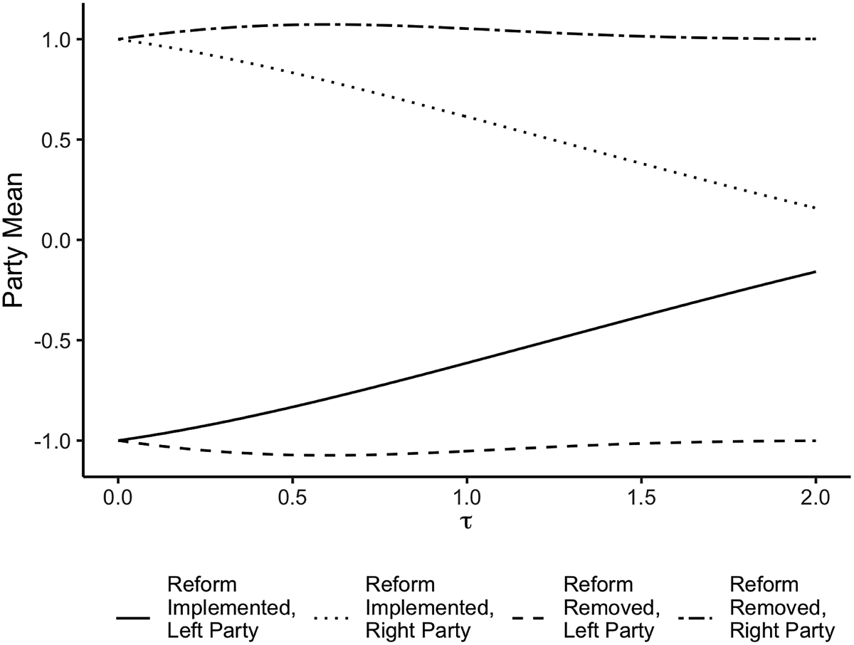
While this result is substantively important and we empirically examine whether it holds in state legislative elections, our primary interest in this result is its implications for how electoral reforms affect aggregate partisan polarization in the legislature. Each party's mean ideology in the legislature is a weighted average of the ideology of the party's incumbents who successfully secure reelection and the challengers who secure a seat. The weights are determined by the incumbent and challenger election rates.Footnote 10 In Figure 3, we plot the locations of each party's mean legislative ideology as a function of the treatment effect magnitude for the different reform scenarios. The figure shows that effects of the reform on each party's ideology are dramatically different depending upon whether the reform is implemented or removed. The magnitude of the change is relatively small when the reform is removed. Additionally, when the reform is removed, there is a non-monotonic relationship between the magnitude of the challenger ideology treatment effect and the party's mean ideology. For sufficiently high treatment effects, the reduction in challenger win probabilities is so dramatic that the party's legislators are almost entirely incumbents.
Mean party ideological positions.

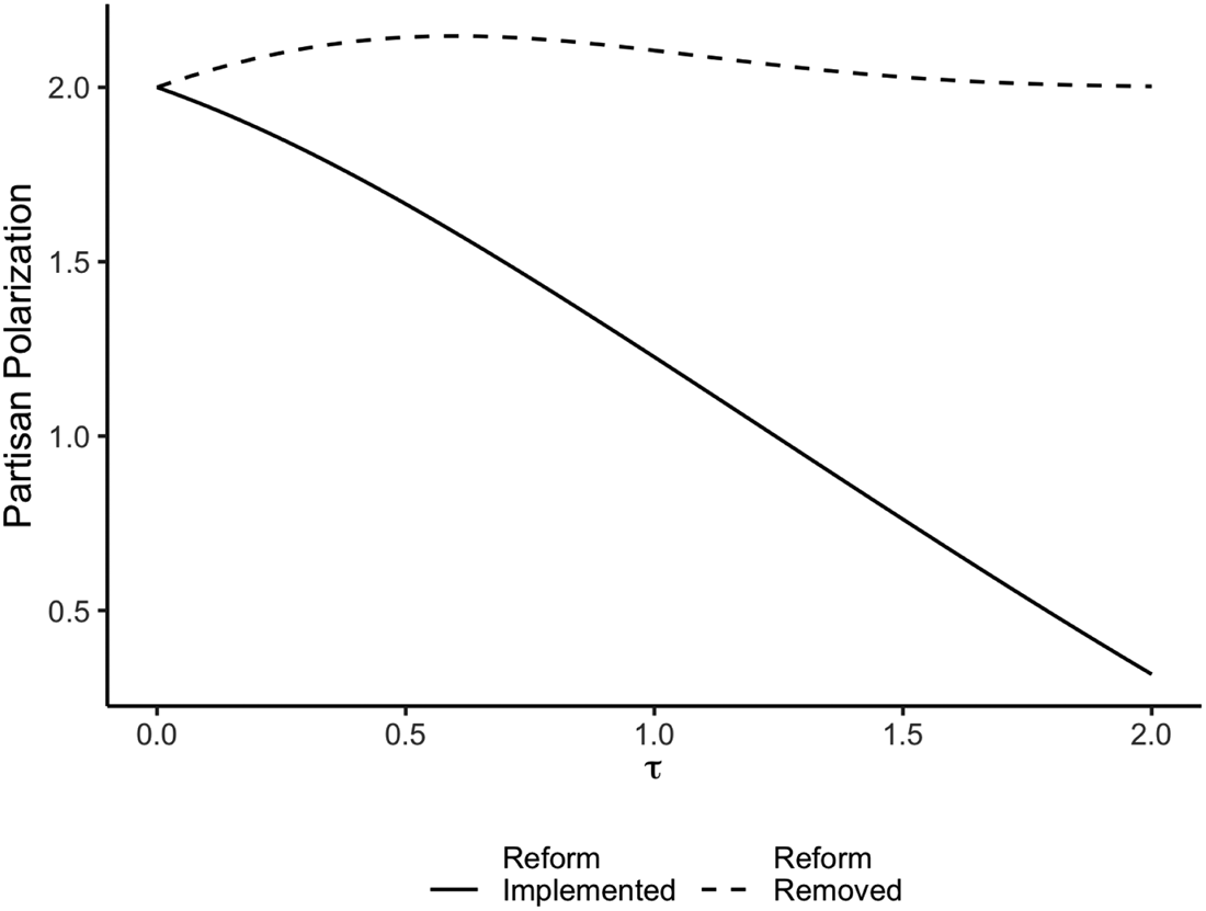
We can now characterize the aggregate level of partisan polarization in the legislature under the different scenarios. Partisan polarization is simply the difference in the mean ideology of the right party's legislators and the left party's legislators. Figure 4 displays these quantities for our two scenarios. While polarization increases when the reform is removed, the effects are quite small in magnitude. To see this directly, we next plot the magnitude of the polarization changes relative to the baseline period.
Partisan polarization.

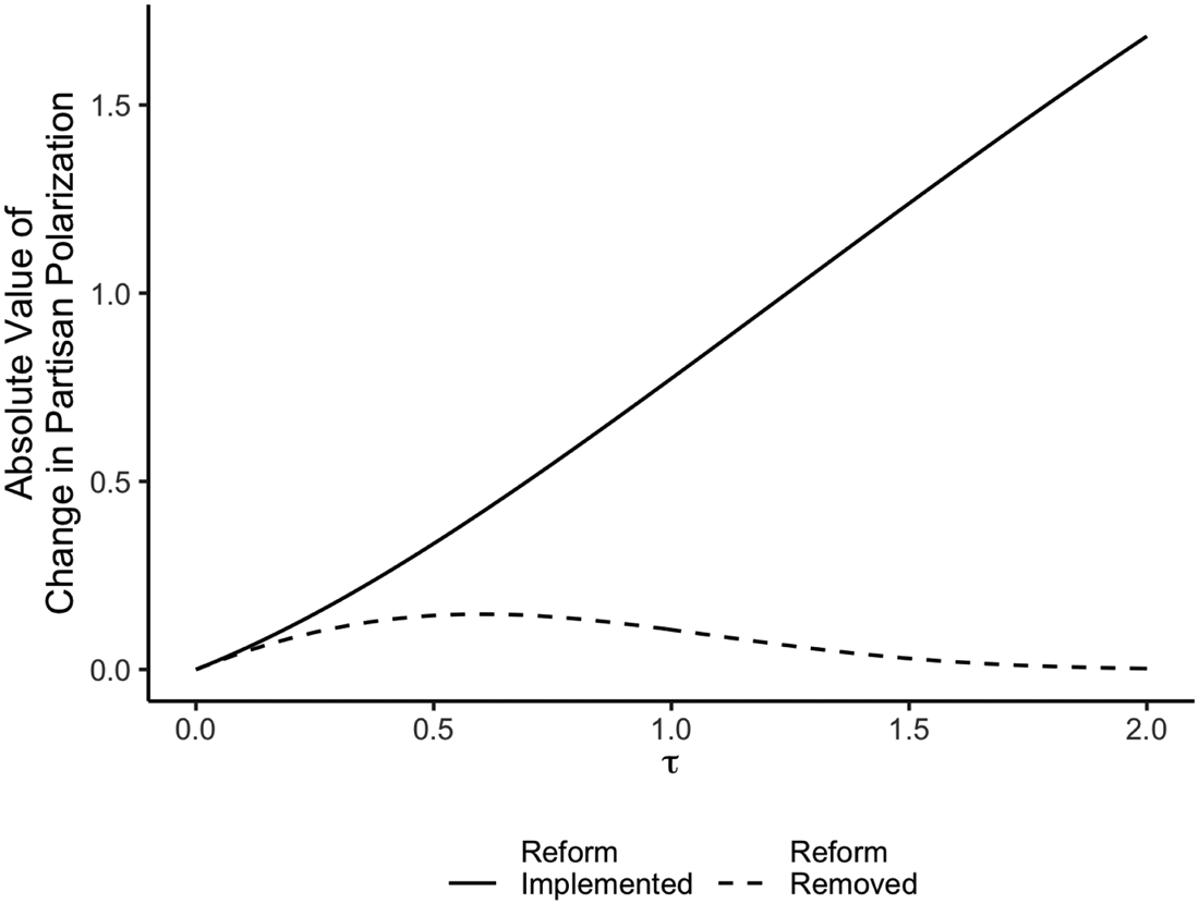
As seen in Figure 5, the magnitudes of the change in polarization are not equivalent when the reform is implemented and removed. The magnitude of the change is always larger when the reform is implemented than removed. We can now express our second result.
Result 2: Expected partisan polarization increases in reform-removing states and decreases in reform-implementing states relative to the baseline period. For a fixed treatment effect size, the magnitude of the change in expected partisan polarization is greater in reform-implementing states than in reform-removing states.
Change in partisan polarization.

In the Online Appendix, we generalize the results from this parametric example. We allow for any spatial component of the utility function that is single-peaked, symmetric, and strictly decreasing in the distance between the voter's ideal point and the candidate's ideology and any preference shocks that are independent and identically distributed with support over the entire real line. We also allow the incumbent to partially adjust her ideological location. Complete incumbent policy persistence is often an unrealistically strong assumption and we show that our results hold whenever there is a friction that prevents incumbents from adjusting completely to their party's challenger position.
Our framework can be extended to allow for subsequent elections. In each period, the expected fraction of incumbents who served in the initial period will decrease as they are defeated by challengers. After many elections, the expected effect of aggregate polarization will converge to the challenger-level treatment effect τ because the fraction of the legislature consisting of candidates who did not serve in the initial period will converge toward 1. This dynamic analysis also makes clear that the replacement rate of initial period incumbents by challengers is an essential variable for understanding how electoral reforms affect polarization.
Result 3: As the number of elections goes to infinity, the change in polarization relative to the baseline period converges to τ.
When estimated on the sample of new entrants to the legislature, the expectation of the estimator of the effect of the electoral reform on polarization is equal to τ so this procedure generates an unbiased estimator for the long-run change in polarization. Of course, this quantity does not allow us to understand the dynamic path of legislative polarization because it ignores both how incumbents adjust their behavior to changing electoral circumstances and the probability that new entrants will replace the baseline period incumbents in the legislature. Below, we discuss how to combine estimates of τ with information on incumbent policy persistence and the replacement rate of incumbents to estimate the dynamic path of aggregate polarization.
Our theoretical framework makes clear that the reelection rate of incumbent legislators is an important factor driving the aggregate polarization consequences of an electoral reform. This insight raises the important issue of how other institutional reforms, such as term limits, that affect the probability that incumbents continue in office, but may not have a direct effect on the policy positions of incumbents and challengers, interact with reforms that change the ideological location of challengers to jointly determine the aggregate level of polarization.
Data description
We combine data from several sources to examine the implications of the theory in the context of campaign contribution limits and polarization in state legislatures. Following Barber (Reference Barber2016), we examine the relationship between changes in PAC contribution limits in state legislative elections and incumbent electoral performance and polarization. Barber (Reference Barber2016) argues that individual donors are ideologically motivated and more likely to support ideologically extreme candidates while PACs are more interested in obtaining access to legislators. As a result, he expects that when candidates are able to receive an unlimited amount of money from PACs, legislators will be less polarized. Using data on campaign finance laws in the US states and measures of state legislator ideology, Barber (Reference Barber2016) finds that in states that allow unlimited PAC contributions, the ideological extremity of legislators in their first term decreases. Meanwhile, in states that allow unlimited contributions from individual donors, first-term legislators are more polarized.
Based on his analysis, we identify the implementation of unlimited PAC contribution limits as a moderation-inducing reform and use his data to identify the presence of PAC campaign contribution limits in each state from 1990 to 2012. We use this information to create the three main independent variables used in our analyses. We first generate an indicator that is equal to one in each year that a state allows unlimited PAC contributions. Then, we create two variables indicating periods in which a state implements unlimited PAC contributions or removes unlimited PAC contributions in order to assess how the effects of electoral reforms vary across these scenarios. The first of these two variables is coded such that it is equal to one for each year after a state switches from having a PAC contribution limit to allowing unlimited PAC contributions.Footnote 11 The second variable is equal to one in each year after a state switches from allowing unlimited PAC contributions to a PAC contribution limit being in place.Footnote 12 Table A.1 in the Online Appendix indicates the states and years that are classified as removing and implementing unlimited PAC contributions.
Our first set of dependent variables are two measures of incumbents’ electoral success. In particular, we generate indicators of whether or not an incumbent runs for reelection and whether or not an incumbent wins the election using the data from Klarner et al. (Reference Klarner, Berry, Carsey, Jewell, Niemi, Powell and Snyder2015). Next, we measure the ideological position of incumbent legislators and challengers using two sources of data. First, we utilize Shor–McCarty scores, which are ideal points that are scaled using legislators’ roll-call votes and bridged across states using candidate responses to the National Political Awareness Test (Shor and McCarty Reference Shor and McCarty2011). Because Shor–McCarty scores are not available for challengers who do not win their election, we also use CF-scores from Bonica (Reference Bonica2016) to measure ideal points of challengers. CF-scores are generated for both incumbents and challengers using campaign contributions (Bonica Reference Bonica2013).Footnote 13
Both of these ideal point measures are polarized such that lower scores indicate that a legislator is more liberal and higher scores indicate that a legislator is more conservative. Zero is an arbitrary neutral point on the ideological scale and does not have a substantive interpretation. We create a dependent variable that measures ideological extremism for our analysis by taking the absolute value of the Shor–McCarty scores and CF-scores so that smaller values of the variable indicate that legislators are more ideologically moderate and larger values indicate that legislators are more ideologically extreme. However, due to a lack of substantive meaning for zero in the Shor–McCarty scores and CF-scores, as the dependent variable decreases, it does not necessarily mean that a legislator is approaching the ideological position of a perfect moderate. As an alternative, we could generate a measure of within-party ideological extremism using a transformed version of the ideology scores. For example, Barber (Reference Barber2016) measures ideological polarization of state legislators by multiplying Shor–McCarty scores by negative one for Democrats and using the original Shor–McCarty scores for Republicans. We use the absolute value of the ideology measures in our main analysis because we are interested in the ideological extremism of legislators regardless of their party affiliation.Footnote 14 We present results in Table A.11 of the Online Appendix with the same measure of the Shor-McCarty scores as Barber (Reference Barber2016) and the results are substantively similar to those presented in the body of the paper.Footnote 15
Using these two sources of data, we create a dataset that includes all incumbent state legislators along with their Shor–McCarty score and CF-score as well as a dataset with all challengers and their CF-score. The coverage of the Bonica (Reference Bonica2016) data begins in 1990 while the Shor and McCarty (Reference Shor and McCarty2011) data starts in 1993. We include the both upper and lower chambers of state legislatures in the sample and exclude multi-member districts. Finally, because term limits affect the rate at which incumbent legislators can be replaced and, consequently, moderate the effects of electoral reforms, we also compile data on the presence of term limits in state legislatures using information from Kousser (Reference Kousser2005) and the National Council of State Legislatures. These data are used to create an indicator equal to one in years in which state legislators are subject to a term limit.
Empirical approach
We examine the central implications of the theoretical framework in the context of an important electoral reform in state legislatures: the implementation and removal of unlimited PAC contributions.Footnote 16 As discussed, Barber (Reference Barber2016) argues that implementing unlimited PAC contributions causes legislators to behave more moderately, because it results in candidates focusing less on obtaining funds from ideologically extreme individual donors. On the other hand, removing unlimited PAC contributions should result in more extreme legislators as they have to appeal to these more extreme individual donors.
Our first specification examines how the level of the dependent variable changes when states have no limits on PAC contributions. Denoting legislatorsFootnote 17 with the subscript l, states with the subscript s, and time period with the subscript t, we first estimate the standard specification with an indicator for whether PAC contributions are unlimited in state s in year t:

The state fixed effects allow for unobserved time-invariant heterogeneity within states and we include time period fixed effects to accommodate differences in the level of the dependent variable across time periods. The above specification cannot identify how treatment effect magnitude varies with whether a PAC contribution limit was implemented or removed. To examine this possibility, we separately include indicators for each of these scenarios in our next specification.

In all of our analyses, we employ heteroskedasticity robust standard errors and cluster the standard errors at the state level because the PAC regulations vary at the state level, not the individual legislator level.
As in Barber (Reference Barber2016), our key identifying assumption is that, after conditioning on state and year fixed effects, the error term is conditionally independent of PAC contribution limit regulations. While the state fixed effects account for time-invariant unobservables, there may be time-varying unobservables that are correlated with the presence of PAC contribution limits. For example, the assumption could be violated if states that are becoming more polarized are more likely to change their PAC contribution regulations. One approach to make this conditional independence assumption more plausible is to allow for trends in the state-specific level of the dependent variable. In each table, we also include the results of a regression specification with a state-specific linear time trend. We also interact the year fixed effects with an indicator for whether the legislator is a Democrat to allow for partisan waves that influence the level of the dependent variable. While these approaches cannot rule out richer dynamics that might confound the relationship between treatment assignment and the outcome of interest, they do give us more confidence in the credibility of our estimates.
Our main analysis of polarization uses a measure of ideology that does not vary within legislators over time. As a result, we cannot directly estimate the extent of incumbent ideological policy persistence and how it responds to changes in PAC contribution regulations.Footnote 18 If legislators do change their ideological behavior in response to electoral reforms, these static measures of legislator ideology will result in underestimates of the magnitude of the treatment effects because some of the change will be averaged across all of the years that the legislator serves in office. Our estimates of polarization effects can be interpreted as lower bounds on the true magnitude.
While our analysis focuses on the influence of PACs on candidates’ ideological positions, unlimited PAC contributions may also have a direct effect on the magnitude of the incumbency advantage. Primarily, access-motivated PACs contribute more of their resources to incumbents than challengers (Fouirnaies and Hall Reference Fouirnaies and Hall2014). Implementing unlimited PAC contributions may moderate challengers, but also increases incumbents’ share of campaign resources. This offsetting factor may be sufficiently large that incumbent reelection rates actually increase after the implementation of unlimited PAC contributions. Our research design does not allow us to disentangle these two effects, but we are able to investigate which effect dominates by examining how incumbent reelection rates change in response to unlimited PAC contributions.
Results
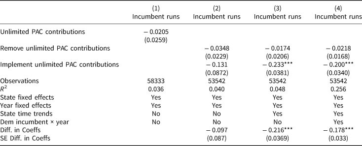
We first examine the relationship between PAC contribution limits and the probability that an incumbent runs for reelection in Table 1, because if moderating electoral reforms induce the entry of more electorally viable challengers, we should observe more voluntary exits from the legislature among incumbents. Column 1 displays the effect of allowing unlimited PAC contributions on the probability that an incumbent runs for reelection. The coefficient on the unlimited PAC contributions variable is negative but is not statistically significant.
Probability incumbent runs for reelection

Heteroskedasticity robust standard errors clustered at the state level in parentheses.
+p < 0.10, *p < 0.05, **p < 0.01, ***p < 0.001.
In Columns 2–4 we estimate the impact of removing and implementing unlimited PAC contributions separately. The model in Column 2 includes state and year fixed effects. Column 3 adds state time trends and Column 4 adds state time trends along with the Democrat incumbent and year fixed effects interaction to the model. Consistent with the theory, we find that when an unlimited PAC contribution policy is implemented, an incumbent is less likely to run for reelection. In particular, according to the models with state time trends, the implementation of unlimited PAC contributions causes a statistically significant 0.200–0.233 decrease in the probability that an incumbent runs for reelection. On the other hand, removing the possibility that a PAC can contribute unlimited funds to a candidate appears to have no effect on if an incumbent runs for office again. To further probe the differential effects of implementing and removing unlimited PAC contributions, we show the difference between the coefficients on the two independent variables of interest in the bottom panel of Table 1. In all three specifications of the model, the coefficient on the variable indicating unlimited PAC contributions limits are implemented is greater in magnitude than the coefficient on the variable indicating unlimited PAC contributions are removed and the difference in coefficients is statistically significant in the models with state time trends.
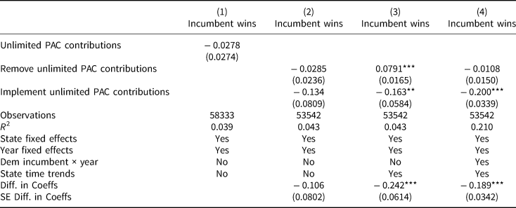
Not only is an incumbent less likely to run for reelection after unlimited PAC contributions are implemented, but she is also less likely to win conditional on running. In Table 2, we regress a variable indicating whether or not an incumbent wins her election on the independent variables of interest. As before, all of the columns include state and year fixed effects while Columns 3 and 4 include state time trends and Column 4 includes a control for if there was a Democratic incumbent in each year. The results indicate that implementing unlimited PAC contributions is associated with a decrease in the probability that an incumbent is reelected, and this effect is statistically significant across the specifications of the model that include state time trends. The estimated effects of removing PAC contribution limits are not consistent across the different specifications of the model. For example, Column 2 of Table 2 indicates that the sign on the coefficient of the removing PAC contributions variable is negative, while in Column 3, we find that the effect of this reform on incumbent reelection rates is statistically significant and positive. In the bottom panel of Table 2, we show that there is a statistically significant difference in the effects of removing and implementing unlimited PAC contributions in the models with state time trends.
Probability incumbent wins reelection

Heteroskedasticity robust standard errors clustered at the state level in parentheses.
+p < 0.10, *p < 0.05, **p < 0.01, ***p < 0.001.
A subtler implication of the theoretical framework is that the effect of implementing the moderation-inducing reform on incumbent reelection rates will decay over time as the old incumbents are replaced by new entrants. When unlimited PAC contributions are implemented, the incumbent reelection rate will decline immediately, but the magnitude of this effect will converge toward 0 as the old incumbents exit office and are replaced by more moderate challengers. In Table A.8 in the Online Appendix, we investigate this prediction by regressing incumbent reelection on an indicator for whether unlimited PAC contributions were implemented before the current election, the previous election, two elections prior, and three elections prior. We find that the largest effects of implementing unlimited PAC contributions are in the current election cycle with a 0.294 decrease in the probability an incumbent is reelected. When this treatment is implemented before the three prior election cycles, the estimated effects are roughly 1/10 of the magnitude of the current election cycle effect. None of the three dynamic treatment effects are statistically distinguishable from 0.
The set of results regarding whether or not an incumbent runs for reelection and incumbent reelection rates provides evidence consistent with Result 1 of the theory. Incumbents are replaced at a faster rate when a moderating reform is implemented compared to when it is removed. To assess how this affects aggregate legislative outcomes, we now turn to an analysis of the effects of implementing and removing unlimited PAC contributions on polarization in state legislatures. Recall that Result 2 of the theory predicts that when a moderation-inducing reform is implemented, which in our context is implementing unlimited PAC contributions, there will be a decrease in partisan polarization and that the effect on polarization will be larger than when a moderation-inducing reform is removed.
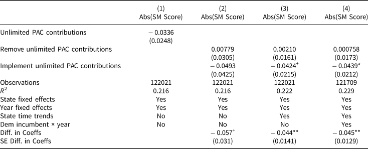
In Table 3, we display the results of models with the absolute value of legislators’ Shor–McCarty scores as the dependent variable.Footnote 19 Consistent with Barber (Reference Barber2016), in Column 1, we find that unlimited PAC contributions lead to less polarized legislators, although the coefficient on this variable is not statistically significant. Turning next to Columns 2–4 of Table 3, we regress the absolute value of legislators’ Shor–McCarty scores on the variables indicating if an unlimited PAC contributions are being implemented or if unlimited PAC contributions are being removed. Across all of the models, the coefficient on the implementing unlimited PAC contributions variable is negative, as expected, though it is only statistically significant after the inclusion of state time trends in Columns 3 and 4. Further, the magnitude of the effect of implementing unlimited PAC contributions is larger than the effect of removing this reform. The difference in the coefficients on these two variables is at least marginally statistically significant across all three specifications of the model, and we find that the change in partisan polarization when unlimited PAC contributions are implemented is 0.044 points to 0.057 points larger than when unlimited PAC contributions are removed.
Polarization

Heteroskedasticity robust standard errors clustered at the state level in parentheses.
+p < 0.10, *p < 0.05, **p < 0.01, ***p < 0.001.
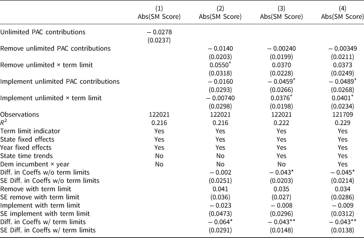
Our theoretical framework also indicates that the effects of an electoral reforms should be moderated by other institutions that influence the likelihood that incumbents are replaced. We investigate how one particular institutional rule, state legislative term limits, moderates the effects of removing and implementing unlimited PAC contributions. In Table 4, we estimate models that include interactions between the new and removed unlimited PAC contributions variables and a variable indicating if a state legislature has term limits. Looking first at the model in Column 2, we find support for our hypothesis that term limits will moderate the effects of unlimited PAC contributions. The interaction of the remove unlimited PAC contributions variable and term limit variable is positive and marginally statistically significant. In the bottom panel of the Table 4, we show that after accounting for the constituent term in the model, the estimated effect of removing a PAC contribution limit in term limit states is positive, though not statistically distinguishable from zero. The difference between removing and implementing this reform in states without term limits is substantively very small and statistically insignificant. However, when term limits are in place, the effect of removing unlimited PAC contributions on the absolute value of legislators’ Shor–McCarty scores is 0.041 and the effect of implementing unlimited PAC contributions is − 0.023. Moreover, the difference in these effects is a statistically significant − 0.064. This indicates that the effects of removing and implementing PAC contribution limits are moderated by other legislative rules, such as term limits, that increase the rate at which incumbents leave office. In the models presented in Columns 3 and 4 of Table 4, we find that the interaction between PAC contribution limit removal and term limits is positive, but the difference in effects is similar across both states with and without term limits.
Polarization and term limit interactions

Heteroskedasticity robust standard errors clustered at the state level in parentheses.
+p < 0.10, *p < 0.05, **p < 0.01, ***p < 0.001.
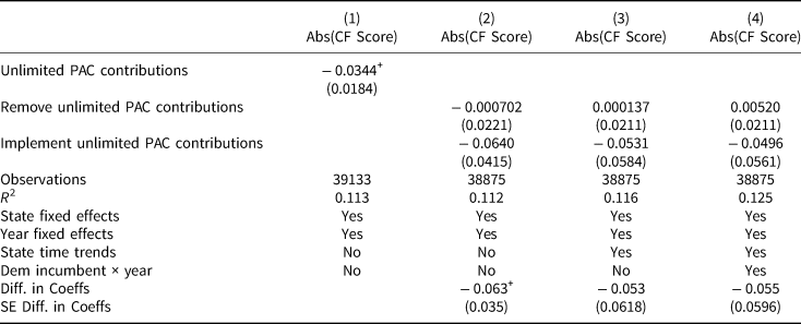
Finally, the results of our theoretical model are driven, in part, by the assumption that moderating electoral reforms induce a pool of challengers that is more ideologically moderate and, consequently, more electorally viable. If this assumption of the theory is correct for this empirical setting, we should also observe more moderate challengers after unlimited PAC contributions are permitted. To test this hypothesis, we estimate models with the ideological polarization of challengers as the dependent variable using the absolute value of challengers’ CF-scores. These results are displayed in Table 5. Looking first at the model in Column 1, we find that unlimited PAC contributions cause more moderate challengers to enter state legislative races. In Columns 2, 3, and 4, we estimate the effects of implementing and removing unlimited PAC contributions on the ideological extremism of challengers. Although the estimates do not achieve standard levels of statistical significance, the coefficients on the implementing PAC contributions variable are negative and substantively similar to the estimated effect of implementing this reform on the ideology of elected legislators (Table 3) across all specifications of the model. Further, the difference in the coefficients shows that implementing unlimited PAC contributions causes a larger change in the ideological position of challengers than removing unlimited PAC contributions.
Challenger polarization

Heteroskedasticity robust standard errors clustered at the state level in parentheses.
+p < 0.10, *p < 0.05, **p < 0.01, ***p < 0.001.
Polarization counterfactuals
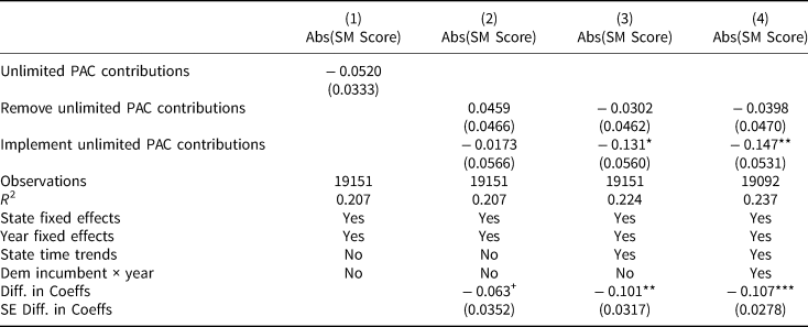
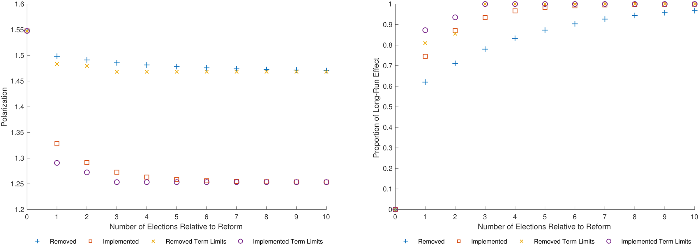
In our final set of analyses, we use the framework to investigate the dynamic path of polarization under alternative counterfactuals. The conventional polarization estimator derived from restring the sample to first-term legislators recovers the long-run effect of polarization, but does not illuminate the dynamic path of polarization across election cycles. We consider the evolution of polarization from the baseline period before the reform through the following ten election cycles under the alternative scenarios of implementing unlimited PAC contributions and removing unlimited PAC contributions with and without term limits. In the Online Appendix, we describe the exact regressions that we estimate and the fitted probabilities and polarization values that form the basis of the counterfactual exercise. The essential idea is that we use the polarization point estimates to construct the baseline level of polarization among old incumbents and the level of polarization among new entrants and then we use the fitted incumbent reelection probabilities to estimate the share of old incumbents and new entrants in the legislature in each period. We use the estimates from Column 4 of Table 6 to measure the long-run effect on the polarization of legislators.
Polarization (first-term legislators only)

Heteroskedasticity robust standard errors clustered at the state level in parentheses.
+p < 0.10, *p < 0.05, **p < 0.01, ***p < 0.001.
While the static measure of legislator ideology that we use does not allow us to estimate the extent of incumbent policy persistence, we can make alternative assumptions about the level of incumbent policy persistence in order to examine how the evolution of partisan polarization varies with incumbent policy persistence. In our first set of results, we assume complete incumbent policy persistence. We then relax this assumption and specify the level of the incumbent policy persistence parameter at 0.5 in the second set of counterfactuals.
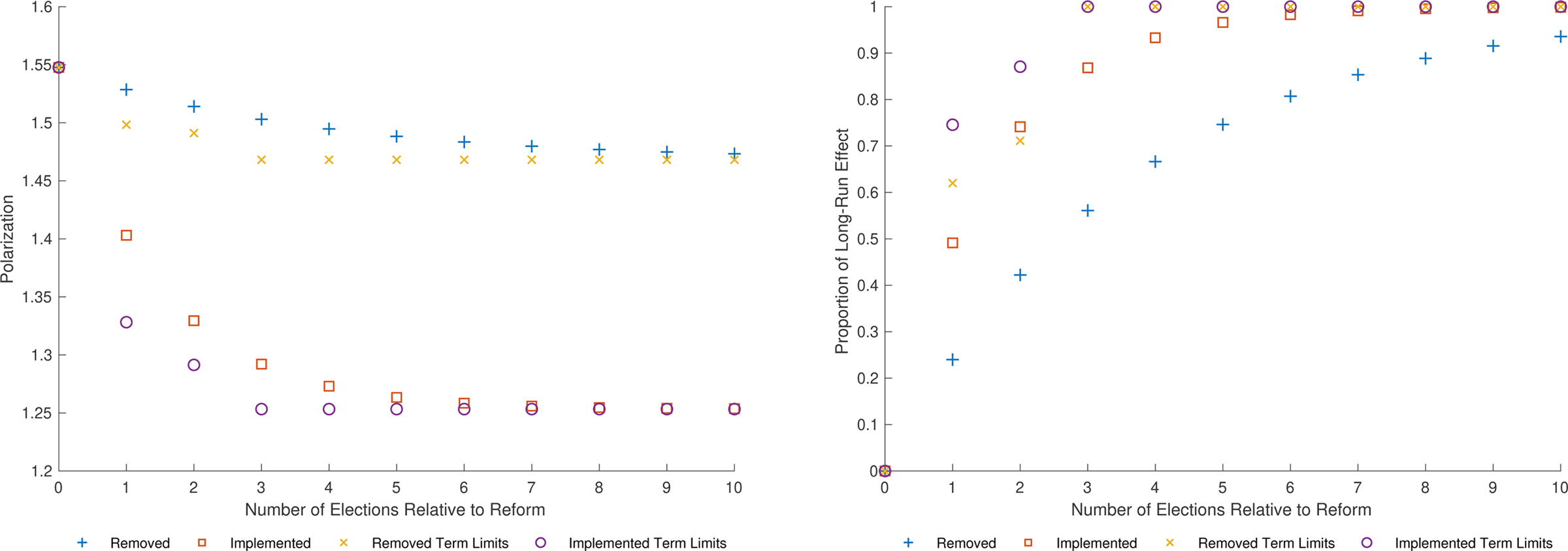
In Figure 6, we present the results of the counterfactual analysis.Footnote 20 In the left panel, we report the evolution of polarization across the electoral cycles for the four different scenarios. The right panel presents the same counterfactuals, but now defines the y-axis as the proportion of the long-run effect after each election cycle. The right panel allows us to directly compare the magnitude of the polarization effects across the four scenarios. The graphs reveal that the dynamic path of polarization differs considerably across the scenarios. After one election, the effect of removing the reform is roughly 25 percent of the total effect while the effect is approximately 50 percent when the reform is implemented. In both term-limited scenarios, the effect magnitudes are dramatically larger relative to the no-term limits case. The effect magnitudes gradually increase in the next period. Starting after election period 3, the term-limited scenarios reach the long-run level of polarization because all of the pre-reform incumbent legislators are forced to exit the legislature and the legislature is entirely composed of new entrants. By election period 4, the reform implemented effect is more than 90 percent of the long-run effect, but the reform removed effect is still about 65 percent of the long-run effect.
Polarization counterfactuals, full incumbent policy persistence: λ = 1.

We now examine counterfactuals under a lower level of incumbent policy persistence. We specify the incumbent policy persistence parameter to 0.5 so that old incumbents adjust their positions to the midpoint of the old incumbent pre-reform ideological position and the new entrant ideological position. While we cannot directly estimate the degree of ideological policy persistence, this level of 0.5 represents a fairly low level of ideological policy persistence and we would expect that in real legislative settings, legislators are unlikely to exhibit such a large adjustment in their ideological policy positions. In Figure 7, we report the polarization counterfactuals with this partial incumbent policy persistence. Now the percentage of the total effect that is reached after the first election is more than 60 percent when the reform is removed and more than 70 percent when it is implemented without term limits. The effect proportions increase steadily over the next several election cycles and the dynamic path of polarization more rapidly approaches the long-run level than in the scenarios with complete policy persistence.
Polarization counterfactuals, partial incumbent policy persistence: λ = 0.5

Conclusion
Using a simple theoretical framework, we have jointly examined how electoral reforms affect incumbent reelection rates, the behavior of challengers, and the behavior of incumbents to determine the aggregate level of polarization in legislative bodies. The framework shows that the dynamic effects of electoral reforms on partisan polarization depend critically upon whether a moderation-inducing reform is implemented or removed. We find empirical support for these predictions in the context of campaign finance reforms in state legislatures. Our analysis and results show how other electoral institutions, such as term limits, interact with reforms that have a more direct effect on the ideological positioning of candidates to jointly influence the level of partisan polarization in a legislature. The framework also motivates examining changes in polarization across repeated cohorts of new entrants as in McGhee et al. (Reference McGhee, Masket, Shor, Rogers and McCarty2014) and Barber (Reference Barber2016) as an estimator for the long-run effects of electoral reforms on polarization.
While the empirical analysis considers only one specific electoral reform, our framework can be used to analyze other electoral reforms, such as changes in redistricting rules (Grainger Reference Grainger2010). Incorporating two-stage elections to examine reforms to primary election rules (McGhee et al. Reference McGhee, Masket, Shor, Rogers and McCarty2014) would also be fruitful. This analysis would enrich our understanding of how electoral institutions affect the level of polarization in legislative bodies. It would also be valuable to extend the counterfactual analysis to other legislative features beyond term limits that affect the probability that pre-reform incumbents remain in office. Other features, such as the level of legislator compensation and private sector outside options affect the probability that legislators remain in office (Diermeier et al. Reference Diermeier, Keane and Merlo2005). Incorporating these features into the counterfactual analysis would improve our understanding of the evolution of partisan polarization over time.
Supplementary material
To view supplementary material for this article, please visit https://doi.org/10.1017/psrm.2020.14.
Acknowledgments
We thank Michael Barber for sharing data and answering our questions on campaign finance regulations. We thank Miguel Rueda, Mona Vakilifathi, Vlad Kogan and participants at MPSA and the Emory PIM seminar for helpful comments.