2. THE CONTROVERSY OVER THE ACCURACY OF COLUMBUS' LOG

Miles H. DavidsonReference Davidson⁷ summarized the popular and highly critical view of the navigational data in the log in stating: “What is evident in the historiography of the first voyage that few have been willing to accept is that the figures in the Diario [Columbus' log] simply do not make sense when studied either individually or collectively. Columbus' hagiographers have developed theories and explanations, most of them highly selective but none of them convincing. Barring discovery of additional sources, the true meaning of these numbers will remain an enigma” (Davidson 1997:212–213, emphasis added). An item that has without foundation contributed to the misunderstanding and confusion in analysis of the data in Columbus' log is the fact that he reported separate and lower figures given to the crew (for fully explained reasons) and reported separate and different estimates of distance given to him by the Spanish pilots. These irrelevant figures have no relationship to Columbus' accurate dead-reckoning figures. Columbus reported these other figures only as a matter of interest and to make his log a complete record of the voyage, not realizing that at some later date they would throw a shadow on the accuracy of his own true dead-reckoning figures. The empirical reconstruction of Columbus' voyage that follows is based solely on Columbus' clear and accurate dead-reckoning data in the log, uncluttered or confused by extraneous, but misleading and patently irrelevant data in the log. Academic scholars with only a superficial knowledge of fifteenth-century navigation do not seem to understand that Columbus' reported magnetic headings “through the water” were not the same as his geographical course “over the bottom” and his distances reported “through the water” were not the same as his geographical distances “over the bottom.” Thus to establish his true geographical course (not heading) and distance “over the bottom” the fifteenth-century magnetic variation and the currents from the North Atlantic Subtropical Gyre must be applied to Columbus' “through the water” figures, a basic navigational procedure that seems to be beyond the capability of academic scholars to comprehend.

3. THE NORTH ATLANTIC SUBTROPICAL GYRE

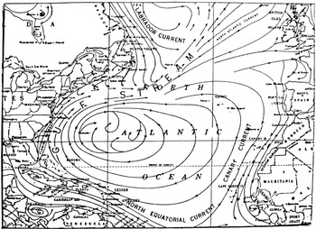
Failure to recognize and apply corrections for the strong ocean currents of the North Atlantic Subtropical Gyre (see Figure 1) has been a major factor contributing to the misunderstanding of Columbus' navigation and log. The North Atlantic clockwise gyre around a slightly mounded Sargasso Sea is set in motion and controlled by forces induced by gravity and the difference in temperature and density of the arctic and tropical waters, balanced against forces arising from the rotation of the earth in what fluid dynamicists call geotropic circulation. These tremendous natural forces have not changed to any measurable degree since Columbus' time so the ocean currents resulting from these forces would also be unchanged.

Figure 1.

The North Atlantic Subtropical Gyre of induced currents showing the westerly current affecting Columbus' 1492 voyage. From NOAA Pilot Chart 1600 series.

Misunderstanding of the unforeseen effect of these strong natural forces on Columbus' track across the Atlantic has contributed to a great extent to the unfounded belief that the navigational data in the log “does not make sense.” This unfounded almost naïve belief exists because the sum total of Columbus' distances reported in the log falls far short of any land or landfall. There is a simple elementary explanation for this seeming incongruity. As an example; from about day 9 to day 27 after leaving Gomera Columbus was carried along by the North Equatorial Current (the southern segment of the North Atlantic Subtropical Gyre) and gained between 7–12 miles each day because of the strong westerly flowing current. Columbus was not aware that he was gaining this induced 7–12 miles which explains why his actual distance covered was far greater than his reported distance in the log. This simple and elementary navigational fact cannot be comprehended by most academic historians who have proposed all manner of invalid explanations for that difference in the log. The manifestly contrived explanations for this difference range from Columbus' alleged gross inability to estimate his speed (and thus determine distance) to preposterous theories about how he was trying to conceal the truth from the Spanish pilots which in turn leads into the equally preposterous theory of the second or secret log.

4. THE LENGTH OF THE NAUTICAL MILE USED BY COLUMBUS

Columbus reported his distance sailed in miles or leagues (four miles) based on his estimate of speed in miles per hour. And further in computing the distance sailed from his estimate of speed in miles per hour it is imperative that we know the length of the standard mile that he was using for his navigation. For my empirical research and reconstruction of Columbus' voyage I used a numerical factor of 2·67 nautical miles to the league which is based on Columbus' use of the Mediterranean 5000 palm mile of 4060 feet to the nautical mile. This factor was established in James E. Kelley's comprehensive study of fifteenth-century navigational measurement standards related to Columbus' voyage (Kelley 1986).Reference Kelley⁸ Kelley's published works on the subject (34 pages including numerous charts and tables of statistical data) is the only scholarly, complete, and creditable study of the subject available to the research historian. Current historians have proposed factors based on unclear Spanish, Portuguese, or even English data for the length of Columbus' league that range from 2·30 to 3·40 nautical miles to the league. And these proposed factors are supported by only a sentence or two asserting the factors are accurate (“speaking from authority”) rather than being supported by a detailed study by a well-qualified and accepted authority on the subject. Kelley's factor of 2·67 nautical miles to Columbus' league was proven accurate when used in the re-sailing and reconstruction of the 1493 return voyage (see Section 6) from a known departure point (Samana Bay) to a known destination (Santa Maria) in a known period of time.

5. FIFTEENTH-CENTURY MAGNETIC VARIATION

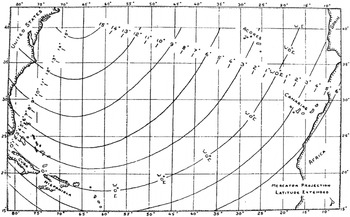
Although the ocean currents were the primary factor influencing the geographical track of Columbus' voyage, the fifteenth-century magnetic variation must be considered to arrive at a true track over the bottom. Both John W. McElroy who manually plotted the entire round trip for Morison in 1941 and Luis Marden who plotted the 1492 westbound voyage in a computer simulation for the National Geographic in 1986, used the Willem van BemmelenReference Van Bemmelen⁹ isogonic lines to correct Columbus' reported compass courses in their plotted tracks. Willem van Bemmelen, a Dutch geophysicist furnished these postulated isogonic lines for the year 1500 (Van Bemmelen 1899) in a paper published in Batavia in 1899. Van Bemmelen's isogonic lines have been largely discredited and since I was unable to find a better source, I developed my own isogonic lines for the period of Columbus' voyage. It is beyond the scope of this study to cover my extensive research (Peck 1993b:58–62) which provided eight geographical points, scattered across the north Atlantic in which the variation for the 1492–1493 time period is known. Placing these areas of known variation on a chart, I then joined them with an extrapolated geometric pattern of isogonic lines which follow the general pattern of the earth's magnetic field. The chart of isogonic lines showing magnetic variation related to Columbus' 1492–1493 voyage is shown in Figure 2, but I hasten to add that it is the new figures of magnetic variation that are important and accurate and the purely schematic lines intended to portray the earth's magnetic field deep within the bowels of the earth are a subject of wide interpretation and are not vitally significant for this presentation of magnetic variation affecting Columbus' voyage.

Figure 2.

Chart of isogonic lines showing magnetic variation related to Columbus' 1492–1493 voyage.

THE TRACK OF COLUMBUS' 1493 RETURN VOYAGE.Reference Peck¹⁰

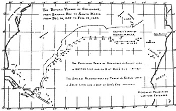
The return voyage from Samana Bay, Hispaniola to Santa Maria in the Azores was sailed and reconstructed first because it contained both a known departure point and a known termination point of the track, thus providing a stable model upon which to test and prove my postulated control factors. This return voyage consisted of 84 legs; a separate leg for each change of magnetic course and distance as covered in a stated time period. Only occasionally did Columbus report his speed in miles per hour which could be related to the reported distance. As explained earlier Columbus' reported distance for each leg was computed from his speed through the water which was considerably different from his speed over the bottom, therefore Columbus' reported distance could be and frequently was far from the geographical distance he sailed over the bottom. I sailed the speed rather than the distance of each leg which then allowed the actual currents to determine the true length or distance in nautical miles over the bottom which is reflected in the reconstructed track shown in Figure 3. I question whether it would be feasible to accomplish this task by manual computation or computer simulation.

Figure 3.

The perceived and actual (reconstructed) 1493 track of Columbus from Samana Bay, Hispaniola to Santa Maria, Azores.

Analysis of the track shown in Figure 3 reveals several instances that confirm Columbus as a masterful and accurate dead-reckoning navigator. To maintain an accurate dead-reckoning course, each change of either heading or speed must be logged and plotted as a separate leg. Columbus certainly did just that. There are 84 separate legs occasioned by either a heading or speed change. Even during the tremendous storm near the end of the voyage, Columbus faithfully logged minor changes in speed or small changes in magnetic headings. The chart in Figure 3 gives a graphic presentation that confirms the accuracy of Columbus' navigation. The lower dotted track was taken directly from the log without any correction factors applied. The upper solid line is the reconstructed track with the correction factors applied.

The total length of the reconstructed track was 2,920 nautical miles which terminated at 37 degrees, 15 minutes North latitude and 24 degrees, 45 minutes West longitude which is about 35 nautical miles east-northeast of Columbus' actual landfall on Santa Maria. This termination point is just a little over one percentage point from Columbus' actual landfall. This 99 percent accuracy for the reconstructed track confirmed that the postulated control factors were essentially accurate and usable and that Columbus' dead-reckoning navigational data as reported in his log was 99 percent accurate.

The reconstructed track of 2,920 nautical miles divided by the 1,085 leagues reported by Columbus equals 2·69 nautical miles to the league that Columbus was using for his navigation and upon which he based his estimate of speed and thus distance. This provides irrefutable mathematical evidence (a difference of only 0·02 mile) that Columbus was using Kelley's Mediterranean or Genoese 5000 palm mile of 2·67 nautical miles to the league. But this evidence to support Kelley's work is at odds with the findings of both David HenigeReference Henige¹¹ and Miles Davidson, two of the foremost and accepted American academic authorities on the voyage of Columbus. In answer to Kelley's statement that; “the Journal data are entirely consistent and highly creditable in a quantitative sense” (Kelley 1985:100), Henige opines; “that these data [in the log or journal] are frequently consistent neither with themselves nor with the real world outside the Diario” (Henige 1991:139), which is stating in a more scholarly manner Davidson's opinion that the data in the log or Diario “does not make sense” (Davidson 1997:212).

With the control factors for Columbus' speed and distance using Kelley's 2·67 nautical miles to the league and the postulated magnetic variation for 1492–1493 (Figure 2) confirmed as essentially accurate by my reconstruction of the 1493 return voyage with a known destination; I now felt confident to use these proven control factors in my reconstruction of the 1492 westbound voyage with an unknown destination.

7. THE TRACK OF COLUMBUS' 1492 VOYAGE FROM GOMERA

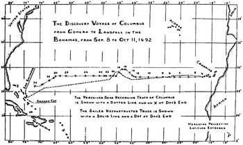
The empirical reconstruction of Columbus' 1492 track from Gomera to landfall on the Indian island of Guanahani was conducted using the same control factors that had been verified in the reconstruction of the 1493 return voyage to Santa Maria. While the study and analysis of the 1493 return voyage was important for obtaining knowledge related to Columbus' navigation and the accuracy of his log it has been the westbound 1492 discovery voyage that has understandably attracted the most attention from historians. Columbus departed the principal port of Gomera on 6 September but for navigational purposes he recorded his departure on 8 September from the westernmost island of Hierro. Columbus later confirmed this when he gave the latitude of Guanahani as due west of Hierro rather than Gomera. My reconstruction of the westbound 1492 voyage also started at Hierro and is labelled as day 1 on the chart in Figure 4.

Figure 4.

The perceived and actual (reconstructed) track of Columbus from Hierro in the Canaries to landfall on the Indian island of Guanahani in the Bahamas.

Columbus would have used a large portolan chart showing the southern coasts of Spain and Portugal, the African coast, and the islands of the Azores, Madeira, the Canaries and Cape Verde, and the rest left blank for plotting his dead-reckoning course to the Indies. The fact that the coast of Africa and the Azores were on Columbus' chart became evident when at one point on the return voyage he indicated his plotted position as south of Flores in the Azores and west of Nafe (Casa Blanca) on the coast of Africa. Figure 4 shows Columbus' plotted track just as it would have appeared on his portolan chart and labelled as: “The Perceived Dead-Reckoning Track of Columbus.” Columbus believed that Cipangu (Japan) and the Indies lay due west from the Canaries so he religiously stuck to that heading for most of the voyage. Delete the modern shorelines on the western edge of Figure 4 as well as the plotted reconstructed track and the remaining chart with Columbus' perceived track (northern dotted line) would be very similar to Columbus' portolan chart from Hierro to landfall on Guanahani (San Salvador).

The reconstructed track ended at 23 degrees, 45·5 minutes North latitude, and 75 degrees, 11·0 West longitude, passing within a few miles of the south cape of San Salvador and ended a few miles beyond. Termination of the westbound track at this point would clearly support San Salvador as the Indian island of Guanahani, Columbus' landfall in the New World. Contrary to what academic “authorities” assert, this analysis of the empirical reconstruction of the 1492 discovery voyage and the 1493 return voyage together with more complete supporting documents (Peck 1989,Reference Peck¹² 1991,Reference Peck¹³ 1993) have scientifically and mathematically proved that Columbus was an accurate dead-reckoning navigator and the navigation data in his log was essentially accurate.

8. THE MANUFACTURED COLUMBUS LANDFALL PROBLEM

The identification and geographical location of the Lucayan island of Guanahani, Columbus' landfall in the Indies, was well-known and not a problem to the Spanish pilots and cartographers in the sixteenth, seventeenth, and well into the eighteenth-century. During this period Spanish pilots regularly sailed through the Lucayans (Bahamas) where Guanahani and the other prominent islands north and south of it were clearly shown on their nautical charts and contained in their nautical ruttiers (Peck 2008:39–45).Reference Peck¹⁴ The Spanish historian Juan Bautista Mun~oz was commissioned in 1779 by King Charles III to write a history of Spain's overseas empire which was published some time later as his Historia del Nuevo Mundo. Mun~oz would have been privy to accurate early charts, maps, and related documents of the area and in his Historia reported the established historical fact that the Bahamas island of Watlings (the present San Salvador) was Columbus' landfall.

But this well established knowledge of the location of Columbus' landfall was lost from view when Martin Fernández Navarrete discovered and published the Bartolomeé de Las Casas summary of Columbus' Diario or log (Navarrete 1825).Reference Navarrete¹⁵ Publication of the newly discovered Columbus' log promoted a flurry of published works by academic scholars with only superficial knowledge of navigation or marine geography that named nine different islands in the Bahamas chain as the landfall island of Columbus (Peck 1996)Reference Peck¹⁶ in his 1492 discovery voyage. The most prominent among these works was an article in the 1986 issue of the National Geographic that named the unlikely Samana Cay as Columbus' landfall island. The National Geographic Society assembled a team of “authorities” that quite ostensibly did not include a valid authority on early navigation, Spanish seafaring history, related marine geography, or related early cartography. After five years of research confined largely to Columbus' unclear and irrelevant wandering cruise through the islands after landfall the National Geographic article concluded: “Christopher Columbus first came to the New World at Samana Cay” (Judge 1986:568).Reference Judge¹⁷

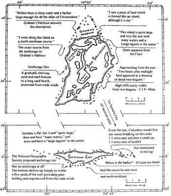
Samana Cay is not only far south of the geographical termination or landfall of Columbus' track from Hierro (Figure 4), but does not begin to answer Columbus' detailed description of Guanahani, the landfall island. Columbus devoted more time (222 lines in his log) in describing the geographical features of Guanahani than he did to any of the subsequent islands he was to discover. His description of the geography and topography, with emphasis on the shoreline, is in minute detail. Columbus described the island as fairly large, level and fertile, with many waters (ponds), a large lake or lagoon in the centre, with several settlements of many people, infers a good protected anchorage on the west side, and stated he followed the coastline from his anchorage in a north-northeasterly direction and found at the north end a large natural harbour surrounded by reefs with a peninsula on one side. The drawings in Figure 5 graphically illustrate how San Salvador has all the geographical features described by Columbus while the small barren and uninhabited Samana Cay has virtually none. It is difficult to understand why the writers of the National Geographic Society did not recognize this strong evidence related to geography, a discipline in which they are well qualified, and instead based their conclusion for Samana Cay primarily on a study of Columbus' navigational log, a discipline in which it is revealed they are poorly qualified.

Figure 5:

Scaled drawings for comparison of geographical features between San Salvador and Samana Cay. Annotations in parenthesis are direct quotes from Columbus' navigation log. From Peck (1993).

9. THE ENIGMA OF COLUMBUS AND CELESTIAL NAVIGATION

There is wide misunderstanding of the role that celestial observations played in the navigation of Columbus and other early pilots. And notice that I used the term “celestial observations” and not the term “celestial navigation.” Celestial navigation as applied to the voyages of Columbus and other early pilots is a misnomer; it is not navigation at all, although by common usage it has assumed that improper name. Dead-reckoning was the only true and accurate navigation system, proven by centuries of reliable documented use, which gave the pilot or navigator a definitive location on his chart and on the face of the earth. A celestial observation whether of the sun or a star gave only an LOP, a line-of-position which is a line cut on the surface of the earth by a plane through the centre of the earth tilted at the sidereal angle of the observed heavenly body with the horizon. The observer knows only that he is somewhere on this infinite line, and thus the celestial observation was of little value to the early pilot for navigation, unless it happened to intersect a dead-reckoning track or known shoreline. This complex interplay between so-called celestial navigation and dead-reckoning is little understood by academic historians, even those accepted as “authorities” on the subject.

Columbus in 1492 was caught up in the early faltering attempts to move celestial observations from the province of learned cosmographers on land to maritime use at sea as a supplement (but not a replacement) of dead-reckoning navigation. In the eight years Columbus spent in Spain awaiting action from the court he would have used the time to read up on cosmology and astrology (the fifteenth-century forerunner of astronomy) primarily to impress the learned men of the Talavera commission that his exploration plan was feasible. He ostensibly obtained a smattering of book knowledge of celestial observations which he voiced when needed but in the application of which he was quite incompetent on his first 1492 voyage.

A quadrant and an astrolabe were placed aboard Columbus' ships by the Spanish crown, but there is no indication that Columbus or any Spanish pilot received instruction of their use before his 1492–1493 voyage. During the Columbian era Spanish ships under government control (i.e. warfare, exploration, and commercial ventures) were outfitted and supplied with stores and equipment by licensed contractors who were paid by the Crown. The quadrant (see Figure 6) and astrolabe put aboard Columbus' vessels were furnished by one such contractor and were placed aboard every vessel regardless of whether the incumbent pilot or master was capable of using the instruments. When Sebastian Cabot became Spain's Piloto Major he attempted to obtain a monopoly on this lucrative trade of furnishing these instruments to the Crown which was challenged in court (Lamb 1969).Reference Lamb¹⁸

Figure 6.

Depiction of a replica of a fifteenth-century quadrant such as used by Columbus in his 1492–1493 discovery voyage.

The first report in the log of Columbus using a quadrant to take a latitude sight on Polaris was on 2 November, 1492 while on the northeastern shore of Cuba. He obtained a reading of 42 degrees from the equinoctial, which is about 1,142 nautical miles too far north, but he dutifully entered it in the log. Morison (1974:73)Reference Morison¹⁹ thought he mistook the unlikely Alfirk for the North Star, but I find that hard to believe since Columbus had earlier indicated complete familiarity with sighting the North Star. In this instance Columbus was manifestly reading the tangent scale on the quadrant instead of the ninety degree elevation (latitude) scale. This is quite possible because the early mariner's quadrant was adapted from the engineer's and surveyor's quadrant which contained several trigonometric scales in addition to the 90 degree elevation scale. As a vital part of my field research reconstructing Columbus' voyage (Peck 1989, 1991, 1993) I made a replica of a fifteenth-century quadrant such as Columbus would have had aboard his ships. This replica of a quadrant is shown in Figure 6 and a close examination of the quadrant reveals that the 42 degree tangent scale of Columbus' reading is adjacent to the 23 degree reading of the 90 degree scale which is reasonably close to Columbus' actual location on the north coast of Cuba.

Columbus realized the 42 degree reading was unreasonable and declared that the quadrant was broken and he would have to get it fixed when he returned to Spain. The quadrant was of course not broken as the only movable part was a small weight hung on a string and actuated by gravity. Columbus simply did not want to admit that he did not know how to properly use the quadrant that had been placed aboard his vessel so he contrived the excuse of a broken quadrant. And none of the Spanish pilots, including the Pinzón brothers questioned Columbus' explanation because they were equally ignorant of the technique of making celestial observations. On 13 December when in Moustique Bay, Haiti, Columbus gave the quadrant one more try and came up with 34 degrees latitude. Once again it is apparent that he was misreading the tangent scale which lines up very closely with the 18 degree latitude scale which in turn was reasonably close to his actual latitude. This second independent reading not only confirms that Columbus was misreading the tangent scale but also indicates that the quadrant in Figure 6 is an accurate depiction of the quadrant used by Columbus on his 1492–1493 voyage.

Although Columbus, as well as other pilots of the period, had little success with making celestial observations at sea, he did use the quadrant to fairly accurately establish the latitude of Jamaica on his fourth voyage. This was manifestly because he had learned to ignore the tangent scale or because he had a later revised marine quadrant that contained only the 90 degree scale. Also this more accurate reading was the result of averaging many observations made over a period of nearly a year from the stable platform of the grounded ships in Jamaica. These ideal conditions did not exist when observations were made at sea. The early cosmographers recognized this need for a stable platform to use the quadrant or astrolabe and thus made their observations on land, noting that; “the roll of the ship could make a difference of four or five degrees” (Taylor 1958:166).Reference Taylor²⁰ Because of this inherent inaccuracy of early celestial observations made at sea, dead-reckoning remained the basic and inherently accurate form of navigation in use for ocean passages well into the seventeenth, eighteenth, and nineteenth centuries. And ocean navigation was not influenced to a significant degree by celestial observations until after introduction of John Davis' reflecting backstaff, the forerunner of the octant and the sextant, together with improved, accurate, and understandable pre-computed tables in the nautical almanacs and manuals of the nineteenth and twentieth centuries.