1. Introduction
Predicting turbulence statistics is a difficult task because of the very large number of scales that exist within any turbulent flow, and the complex way the energy is shifted between different scales, thus making any theoretical analysis extremely challenging. The problem of turbulence is that it has neither simple nor unique solutions. Consequently, one is forced to introduce a series of approximations or hypotheses regarding the structure, dynamics and regimes of turbulent flows. The first approximation, which is an idealization of turbulence, assumes that turbulence is homogeneous and isotropic (HIT). Such an idealization simplifies the problem considerably and, when combined with the hypothesis of self-preservation (the second idealization of the behaviour of turbulent flows, and hereafter denoted SP), allows the achievement of significant theoretical results. SP occurs when the turbulent statistical quantities evolve in a self-similar manner when scaled by suitably chosen length and velocity scales. Despite the enormous theoretical, experimental and numerical efforts over many decades of research, no general consensus has emerged regarding SP. The major drawback relates to the choice of the velocity and length scales. For example, in the early studies of SP, it was common to use either the Kolmogorov velocity and length scales or the combination of turbulence intensity and the Taylor microscale (for an extended review on the subject until the 1970s, see Monin & Yaglom Reference Monin and Yaglom1975). Barenblatt & Gavrilov (Reference Barenblatt and Gavrilov1974) proposed a theory which does not assume single velocity and length scales. George (Reference George1992) later adopted Barenblatt & Gavrilov’s (Reference Barenblatt and Gavrilov1974) approach to develop a theory, arguing that the turbulence intensity and Taylor microscale are the only scales that allow SP to be achieved at all scales of motion. However, the theory fails to predict the decay when turbulence approaches its final stage. Furthermore, George implicitly assumes that the velocity spectrum is self-similar at all wavenumbers (i.e. all scales of motion). This is yet to be observed either experimentally or numerically.
Recently, Meldi & Sagaut (Reference Meldi and Sagaut2013, hereafter denoted MS13), carried out a numerical simulation of Lin’s equation for decaying HIT based on the eddy-damped quasi-normal Markovian (EDQNM) model, extending the work of Clark & Zemach (Reference Clark and Zemach1998). They investigated the decay with the Taylor microscale Reynolds number varying from
 $10^{-4}$
to
 $10^{5}$
for several initial energy spectra,
 $E(k)_{k\rightarrow 0}\sim k^{{\it\sigma}}$
, where
 $E(k)$
is the three-dimensional (3D) energy spectrum and
 $k$
is the wavenumber. Of interest are the cases when
 ${\it\sigma}=1$
, 2 and 4, which are usually referred to, respectively, as exactly self-preserving (
 ${\it\sigma}=1$
, hereafter denoted ESP), Saffman (Saffman Reference Saffman1967b
) (
 ${\it\sigma}=2$
) and Batchelor (Batchelor Reference Batchelor1948 or Kolmogorov Reference Kolmogorov1941b
) (
 ${\it\sigma}=4$
) decaying HIT and correspond to a kinetic energy power-law exponent (
 $k^{2}\sim t^{n}$
)
 $n$
of
 $-1$
,
 $-1.2$
and
 $-10/7$
, respectively. Their results showed that, except for ESP,
 $n$
decreases from
 $n_{init}$
at a very large Reynolds number to
 $n_{final}$
when the Reynolds number is very small. This seems to contradict the result of Speziale & Bernard (Reference Speziale and Bernard1992) who, using a fixed point analysis, showed that
 $n=-1$
is the asymptotically consistent high-Reynolds-number solution. The EDQNM results also conflict with George’s (Reference George1992) theory. For example, they showed that
 $|S_{(\partial u/\partial x)}|$
, the velocity derivative skewness, does not present any increase throughout the entire period of decay, in contrast to George’s analysis which yielded
 $|S_{(\partial u/\partial x)}|\sim R_{{\it\lambda}}^{-1}$
, at least in the initial period of the decay. The EDQNM results also showed that
 ${\it\lambda}$
is not a scaling length, as reflected in the non-collapse of the
 ${\it\lambda}$
-normalized energy spectra, contradicting George’s (Reference George1992) claim that
 ${\it\lambda}$
is the only appropriate scaling length that leads to SP at all scales. Unfortunately, MS13 did not comment on the scaling of the energy transfer term,
 $T(k)$
. They find however that
 $S_{(\partial u/\partial x)}=\text{constant}$
in the initial period, suggesting that
 $T(k)$
scales with
 $u^{\prime 3}$
(
 $u^{\prime }$
is the root-mean-square, r.m.s., velocity). Interestingly, when
 $n\neq -1$
, the EDQNM data show that
 $T(k)$
does not scale with
 $u^{\prime 2}{\it\nu}/{\it\lambda}$
, which is proportional to
 $u^{\prime 3}/R_{{\it\lambda}}$
, the scaling parameter proposed by George (Reference George1992).
Extending and completing the work of Oberlack (Reference Oberlack2002), Oberlack & Zieleniewicz (Reference Oberlack and Zieleniewicz2013) used a Lie symmetry group analysis to tentatively unify all scaling laws of decaying HIT under the same concept. The analysis, which successfully recovered existing decaying laws, seemed to confirm the possibility of an infinite number of integral invariants, and the dependence of
 $n$
on the initial conditions. However, the analysis is valid for very large Reynolds number and uses
 $u^{\prime }$
and the integral length as the scaling variables, which restricts the generality of the results. Oberlack & Zieleniewicz (Reference Oberlack and Zieleniewicz2013) identified an important question, i.e. what scaling parameter is related to a given initial condition? While George (Reference George2012) discussed the issue of the importance of the initial conditions on the decay of turbulence in some special cases, there is still no clear link between the initial conditions and, for example, the scaling parameters or
 $n$
. Further, George (Reference George2012) states that despite our recognition that the effects of the initial conditions persist during the decay, our theoretical understanding of how they persist is lacking.
In this paper, we establish a general framework of SP. Although no new SP solutions are proposed, the framework allows previous SP analyses to be appraised objectively, and explains apparently conflicting claims that have arisen from these analyses. It further provides SP constraints against which experimental or numerical data can be compared to assess whether SP is reached or not. We also address the possible relationship between the initial conditions and the decay of turbulence. In § 2, we develop the theoretical framework of SP valid for all scales of motion and discuss the decay laws for HIT that ensue from the SP analysis. In § 3, we test the analysis against the EDQNM data of MS13, while in § 4, we use the present SP framework to identify unambiguously the assumptions that have been made in earlier analyses. Finally, in § 5 we test the SP analysis against a selection of experimental data of grid turbulence.
2. Theoretical considerations
2.1. Self-preservation
Following Lin’s (Reference Lin1948) approach, which was applied to velocity correlations, we assume that the velocity increment
 $({\rm\Delta}u)=(u(x,t)-u(x+r,t))$
satisfies SP. While Lin’s starting point was the Kármán & Howarth (Reference Kármán and Howarth1938) (hereafter KH) equation for the velocity correlation functions, we consider the two-point transport equation of
 $\langle ({\rm\Delta}u)^{2}\rangle$
for HIT (e.g. Antonia et al.
Reference Antonia, Smalley, Zhou, Anselmet and Danaila2003):
 $$\begin{eqnarray}6{\it\nu}\frac{\partial \langle ({\rm\Delta}u)^{2}\rangle }{\partial r}-\langle ({\rm\Delta}u)^{3}\rangle -\frac{3}{r^{4}}\int _{0}^{r}s^{4}\frac{\partial \langle ({\rm\Delta}u)^{2}\rangle }{\partial t}\,\text{d}s=\frac{4}{5}\langle {\it\epsilon}\rangle r,\end{eqnarray}$$
where
 ${\it\nu}$
is the fluid kinematic viscosity,
 $\langle {\it\epsilon}\rangle$
is the mean turbulent kinetic energy dissipation rate, and
 $r$
the separation along a direction
 $x$
(the angle brackets represent ensemble averages). Equation (2.1), first written in this form by Saffman (Reference Saffman and Zabusky1968), relates the second- to the third-order structure function at all separations. The first, second and third terms on the left-hand side of (2.1) represent the energy contributions from the smallest to the largest scales. The term on the right-hand side represents the energy dissipation.
Following Barenblatt & Gavrilov (Reference Barenblatt and Gavrilov1974), we assume that
 $\langle ({\rm\Delta}u)^{2}\rangle$
and
 $\langle ({\rm\Delta}u)^{3}\rangle$
can be expressed as
 $$\begin{eqnarray}\displaystyle & \langle ({\rm\Delta}u)^{2}\rangle ={\it\delta}u_{2}(t)f(r^{\ast }), & \displaystyle\end{eqnarray}$$
 $$\begin{eqnarray}\displaystyle & \langle ({\rm\Delta}u)^{3}\rangle ={\it\delta}u_{3}(t)g(r^{\ast }), & \displaystyle\end{eqnarray}$$
 $r^{\ast }=r/l(t)$
,
 $l(t)$
,
 ${\it\delta}u_{2}(t)$
and
 ${\it\delta}u_{3}(t)$
are the length and velocity scaling functions to be determined;
 $f$
and
 $g$
are dimensionless functions independent of time. In this formulation, it is not assumed that
 ${\it\delta}u_{3}={\it\delta}u_{2}^{3/2}$
. Barenblatt & Gavrilov (Reference Barenblatt and Gavrilov1974) referred to this type of formulation as ESP and applied it to the second- and third-order velocity correlation functions in the KH equation. George (Reference George1992) also used this type of formulation to apply SP to the spectral energy equation. For convenience, we hereafter drop the dependence on the variable
 $t$
. We refrain from stipulating from the outset the forms that
 ${\it\delta}u_{2}$
and
 ${\it\delta}u_{3}$
take, although it is evident they must have dimensions of velocity squared and velocity cubed, respectively. Of course, one could be tempted to take
 ${\it\delta}u_{2}=u^{\prime 2}$
(the prime denotes an r.m.s. value) on the basis that
 $\langle ({\rm\Delta}u)^{2}\rangle =2u^{\prime 2}-2B_{uu}=0$
(
 $B_{uu}=\langle u(x)u(x+r)\rangle$
) when
 $r=0$
. This however, as we will see later, derives from an SP constraint applied to
 $B_{uu}$
. Thus, for the sake of generality we refrain from assuming
 ${\it\delta}u_{2}=u^{\prime 2}$
. We also depart from earlier analyses by expressing
 $\langle ({\rm\Delta}u)^{3}\rangle$
in terms of
 $\langle ({\rm\Delta}u)^{2}\rangle$
by introducing the velocity increment skewness
 $S$
:
 $$\begin{eqnarray}\langle ({\rm\Delta}u)^{3}\rangle =S\langle ({\rm\Delta}u)^{2}\rangle ^{3/2},\end{eqnarray}$$
which, with the use of (2.2), leads to
 $$\begin{eqnarray}\langle ({\rm\Delta}u)^{3}\rangle =S{\it\delta}u_{2}(t)^{3/2}[f(r^{\ast })]^{3/2}.\end{eqnarray}$$
Obukhov (see Monin & Yaglom Reference Monin and Yaglom1975, p. 403) used (2.4) with
 $S$
constant as a closure model for
 $\langle ({\rm\Delta}u)^{3}\rangle$
. If (2.2) and (2.3) are satisfied then S can also be expressed in an SP form, viz.
 $$\begin{eqnarray}S=c(t){\it\phi}(r^{\ast }),\end{eqnarray}$$
where
 $c(t)$
is a function of time and
 ${\it\phi}(r^{\ast })$
a function of
 $r^{\ast }$
only; both
 $c(t)$
and
 ${\it\phi}(r^{\ast })$
are dimensionless. One can easily identify
 $c(t)$
with
 ${\it\delta}u_{3}/{\it\delta}u_{2}^{3/2}$
and
 ${\it\phi}$
with
 $g/f^{3/2}$
.
We now substitute (2.2) and (2.5) in (2.1) which leads to
 $$\begin{eqnarray}6f^{\prime }(r^{\ast })-\frac{c{\it\delta}u_{2}^{1/2}l}{{\it\nu}}{\it\phi}(r^{\ast })f(r^{\ast })^{3/2}-\frac{3l^{2}}{{\it\nu}{\it\delta}u_{2}}\frac{\partial {\it\delta}u_{2}}{\partial t}\frac{{\it\Gamma}_{1}}{r^{\ast 4}}+\frac{3}{{\it\nu}}l\frac{\partial l}{\partial t}\frac{{\it\Gamma}_{2}}{r^{\ast 4}}=\frac{4}{5}\langle {\it\epsilon}\rangle \frac{l^{2}}{{\it\nu}{\it\delta}u_{2}}r^{\ast },\end{eqnarray}$$
where
 $$\begin{eqnarray}\displaystyle & \displaystyle {\it\Gamma}_{1}=\int _{0}^{r^{\ast }}s^{\ast 4}f(s^{\ast })\,\text{d}s^{\ast }, & \displaystyle\end{eqnarray}$$
 $$\begin{eqnarray}\displaystyle & \displaystyle {\it\Gamma}_{2}=\int _{0}^{r^{\ast }}s^{\ast 5}f^{\prime }(s^{\ast })\,\text{d}s^{\ast }, & \displaystyle\end{eqnarray}$$
 $s^{\ast }$
is a dummy variable of integration. Equation (2.7) holds at all scales if
 ${\it\Gamma}_{1}\sim r^{\ast 5}$
and
 ${\it\Gamma}_{2}\sim r^{\ast 5}$
when
 $r^{\ast }\rightarrow \infty$
. Since
 $f(r^{\ast })\rightarrow \text{constant}$
and
 $f^{\prime }(r^{\ast })\rightarrow 0$
when
 $r^{\ast }\rightarrow \infty$
, it is easy to show that these conditions are satisfied. Note also that both experimental and numerical evidence shows that when
 $r\ast \rightarrow 0$
,
 $f\sim r^{\ast 2}$
. Thus,
 ${\it\Gamma}_{1}\sim r^{\ast 7}$
and
 ${\it\Gamma}_{2}\sim r^{\ast 7}$
and approach zero more rapidly than
 $r^{\ast 4}$
.
SP implies
 $$\begin{eqnarray}\displaystyle & cR_{l}=C_{1}, & \displaystyle\end{eqnarray}$$
 $$\begin{eqnarray}\displaystyle & \displaystyle \frac{l^{2}}{{\it\nu}{\it\delta}u_{2}}\frac{\partial {\it\delta}u_{2}}{\partial t}=C_{2}, & \displaystyle\end{eqnarray}$$
 $$\begin{eqnarray}\displaystyle & \displaystyle \frac{l}{{\it\nu}}\frac{\partial l}{\partial t}=C_{3}, & \displaystyle\end{eqnarray}$$
 $$\begin{eqnarray}\displaystyle & \displaystyle \langle {\it\epsilon}\rangle \frac{l^{2}}{{\it\nu}{\it\delta}u_{2}}=C_{4}, & \displaystyle\end{eqnarray}$$
 $$\begin{eqnarray}R_{l}=\frac{{\it\delta}u_{2}^{1/2}l}{{\it\nu}}\end{eqnarray}$$
may be thought of as a scaling Reynolds number. SP requires
 $C_{1}$
–
 $C_{4}$
to be constant, i.e. independent of
 $t$
, since the coefficient of the first term in (2.7) is constant. If one assumes that
 $R_{l}$
is very large, one may be tempted to drop the first term in (2.7) at all scales. This would be quite incorrect since neglecting the effect of viscosity would, strictly, also lead to removing the dissipation term. Note though that for a given Reynolds number one may carry out an order-of-magnitude analysis on (2.7), which may lead, for example, to neglecting the first term on the left-hand side when considering the large scales only. Alternatively, neglecting the third and fourth terms on the left-hand side amounts to focusing on the small scales. In both cases, the SP analysis would be restricted to a limited range of scales. For example, by neglecting the first term, SP would imply that the ratios
 $$\begin{eqnarray}cR_{l}:\frac{l^{2}}{{\it\nu}{\it\delta}u_{2}}\frac{\partial {\it\delta}u_{2}}{\partial t}:\frac{l}{{\it\nu}}\frac{\partial l}{\partial t}:\langle {\it\epsilon}\rangle \frac{l^{2}}{{\it\nu}{\it\delta}u_{2}}\end{eqnarray}$$
must be constant. Similarly, by considering only the small scales, SP implies
 $$\begin{eqnarray}\displaystyle & cR_{l}=C_{1,sc}, & \displaystyle\end{eqnarray}$$
 $$\begin{eqnarray}\displaystyle & \displaystyle \langle {\it\epsilon}\rangle \frac{l^{2}}{{\it\nu}{\it\delta}u_{2}}=C_{4,sc}, & \displaystyle\end{eqnarray}$$
 $C_{1,sc}$
and
 $C_{4,sc}$
are constant. Note that selecting
 $l={\it\eta}=({\it\nu}^{3}/\langle {\it\epsilon}\rangle )^{1/4}$
and
 ${\it\delta}u_{2}^{1/2}=v_{K}=({\it\nu}\langle {\it\epsilon}\rangle )^{1/4}$
, where
 ${\it\eta}$
and
 $v_{K}$
are the Kolmogorov (Reference Kolmogorov1941a
) length and velocity scales, respectively, yields
 $c=C_{1,sc}$
and
 $C_{4,sc}=1$
, showing that SP is only satisfied at small scales when Kolmogorov scaling parameters are used.
Since we seek SP for all separations
 $r^{\ast }$
, then
 $C_{1}$
–
 $C_{4}$
must also be independent of
 $r^{\ast }$
. Note that if
 ${\it\delta}u_{2}=u^{\prime 2}$
with
 $u^{\prime 2}=(2/3)k$
(
 $k$
is the turbulent kinetic energy) and
 $l={\it\lambda}$
then
 $$\begin{eqnarray}\langle {\it\epsilon}\rangle \frac{{\it\lambda}^{2}}{{\it\nu}u^{\prime 2}}=C_{4}=15\end{eqnarray}$$
since
 ${\it\lambda}^{2}=15{\it\nu}(u^{\prime 2}/\langle {\it\epsilon}\rangle )$
by definition.
To seek a general formulation for
 $l$
, we form the ratios
 $$\begin{eqnarray}\frac{l^{2}}{{\it\nu}{\it\delta}u_{2}}\frac{\partial {\it\delta}u_{2}}{\partial t}:\frac{l}{{\it\nu}}\frac{\partial l}{\partial t},\end{eqnarray}$$
and with
 $(l^{2}/{\it\nu}{\it\delta}u_{2})(\partial {\it\delta}u_{2}/\partial t):(l/{\it\nu})(\partial l/\partial t)=p$
, we find
 $$\begin{eqnarray}{\it\delta}u_{2}={\it\delta}u_{2}(t_{init})\left(\frac{l}{l_{init}}\right)^{p}.\end{eqnarray}$$
Now using the ratio
 $$\begin{eqnarray}\frac{l}{{\it\nu}}\frac{\partial l}{\partial t}:cR_{l}\end{eqnarray}$$
we can, for example, easily obtain
 $$\begin{eqnarray}l^{(2-p)/2}=\frac{(2-p)}{2}q\left(\frac{{\it\delta}u_{2,init}}{l_{init}^{p}}\right)^{1/2}\int _{t_{init}}^{t}c(s)\,\text{d}s+l_{init}^{(2-p)/2}.\end{eqnarray}$$
Interestingly, solutions (2.19) and (2.21) can be seen to correspond to the case
 ${\it\nu}\rightarrow 0$
since they are obtained without applying the SP constraints to the viscous and dissipation terms (first term on the left and the right-hand term of (2.7), respectively). Accounting for these constraints, we can now solve (2.12) which yields
 $$\begin{eqnarray}\displaystyle & l^{2}=2C_{3}{\it\nu}(t-t_{init})+l_{init}^{2}, & \displaystyle\end{eqnarray}$$
 $$\begin{eqnarray}\displaystyle & l^{2}=2C_{3}{\it\nu}(t-t_{init}+l_{init}^{2}/2C_{3}{\it\nu})=2C_{3}{\it\nu}(t-t_{0}). & \displaystyle\end{eqnarray}$$
 $p=-2$
. For the sake of generality, we set the initial condition
 $l=l_{init}$
when
 $t=t_{init}$
(
 $=0$
for example), which allows us to define a virtual origin
 $t_{0}=t_{init}-l_{init}^{2}/(2C_{3}{\it\nu})$
.
If we substitute (2.22b ) into (2.11) and solve, we have
 $$\begin{eqnarray}{\it\delta}u_{2}=B_{n}(t-t_{0})^{n}={\it\delta}u_{2}(t_{init})\left(\frac{l^{2}}{l_{init}^{2}}\right)^{n},\end{eqnarray}$$
where
 $n=(C_{2}/2C_{3})$
, and
 $B_{n}={\it\delta}u_{2}(t_{init})(2{\it\nu}C_{3}/l_{init}^{2})^{n}$
is a constant of integration. Alternatively, using (2.10), (2.14) and (2.22b
), we have
 $$\begin{eqnarray}{\it\delta}u_{2}=\frac{C_{1}^{2}{\it\nu}}{2C_{3}c^{2}}(t-t_{0})^{-1},\end{eqnarray}$$
which has the advantage of eliminating
 $n$
from the expression for
 ${\it\delta}u_{2}$
(notice that when
 $t=t_{init}$
,
 ${\it\delta}u_{2}<\infty$
, unless
 $l_{init}=0$
). It is evident that the conditions (2.10)–(2.12) must be satisfied simultaneously if we seek SP for all
 $r^{\ast }$
. Thus, combining (2.10)–(2.12) and (2.14) and after some trivial manipulation using (2.22b
) we obtain,
 $$\begin{eqnarray}n=\frac{C_{2}}{2C_{3}}=-1-2(t-t_{0})\frac{1}{c}\frac{\text{d}c}{\text{d}t},\end{eqnarray}$$
or, by substituting (2.10) in (2.25),
 $$\begin{eqnarray}n=-1+2(t-t_{0})\frac{1}{R_{l}}\frac{\text{d}R_{l}}{\text{d}t}.\end{eqnarray}$$
Note that if
 ${\it\delta}u_{3}\sim {\it\delta}u_{2}^{3/2}$
then
 $c$
is a constant, which leads to
 $n=-1$
. Thus, if one uses the same scaling velocity (i.e.
 ${\it\delta}u_{3}^{1/3}={\it\delta}u_{2}^{1/2}$
) in (2.2) and (2.3) then the only possible value for
 $n$
resulting from the SP analysis is
 $-1$
, regardless of the Reynolds number. Also,
 $n$
is constant but different from
 $-1$
when
 $(1/c)(\text{d}c/\text{d}t)\sim (t-t_{0})^{-1}$
or
 $(1/R_{l})(\text{d}R_{l}/\text{d}t)\sim (t-t_{0})^{-1}$
(or equivalently
 $c\sim (t-t_{0})^{-(n+1)/2}$
and
 $R_{l}\sim (t-t_{0})^{(n+1)/2}$
). Interestingly, substituting the latter form of
 $c$
into (2.24) and combining it with the expression for
 ${\it\delta}u_{3}$
, we find
 ${\it\delta}u_{3}\sim (t-t_{0})^{n-1/2}$
, in agreement with Barenblatt & Gavrilov (Reference Barenblatt and Gavrilov1974).
Before proceeding with the SP analysis, it is worth commenting on the above results.
(a) The solution for
 $l$
(obtained via (2.12)) is independent of
 ${\it\delta}u_{2}$
. On the other hand
 ${\it\delta}u_{2}$
is constrained by
 $l$
via (2.10) and/or (2.11). This implies that
 ${\it\delta}u_{2}$
cannot be selected independently of
 $l$
and not before
 $l$
is first determined via (2.12). At this stage of the analysis, it is important to stress that
 ${\it\delta}u_{2}$
and
 $l$
are not, a priori, identified with
 $u^{\prime 2}$
and
 ${\it\lambda}$
, respectively. One may however expect that they are related and their relationship should lead to the decay laws for HIT. It is relevant to point out that the use of (2.11) for obtaining
 ${\it\delta}u_{2}$
is more appropriate than (2.10) for describing the decay at all times. Indeed, the use of (2.10) would limit the solutions to the decay period where
 $\langle ({\rm\Delta}u)^{3}\rangle \neq 0$
, that is before the final period is reached.
(b) From expression (2.23) we can write
 $$\begin{eqnarray}{\it\delta}u_{2}l^{-2n}={\it\delta}u_{2}(t_{init})l_{init}^{-2n}=\text{constant},\end{eqnarray}$$
which is an invariant and illustrates the interrelation between SP and the existence of invariants. Using a dimensional argument, Antonia et al. (Reference Antonia, Lee, Djenidi, Lavoie and Danaila2013) proposed the invariant
 $u^{\prime 2}{\it\lambda}^{-2n}=\text{constant}$
for the initial period of decay of HIT, which was supported by their experimental data in a passive grid turbulence. We will show later that
 $u^{\prime 2}{\it\lambda}^{-2n}=\text{constant}$
can be a good approximate of (2.27) in the initial period and when the decay time is not too long. Note that while similar in form to that of Antonia et al. (Reference Antonia, Lee, Djenidi, Lavoie and Danaila2013), (2.27) is an exact expression obtained from the SP analysis, which removes any ambiguity in the selection of both the velocity and length scales. Common invariants in the initial period are
 $u^{\prime 2}L^{5}=\text{constant}$
(Kolmogorov Reference Kolmogorov1941a
,Reference Kolmogorov
b
) and
 $u^{\prime 2}L^{3}=\text{constant}$
(Saffman Reference Saffman1967a
,Reference Saffman
b
) where
 $L$
is the integral length scale. However, Vassilicos (Reference Vassilicos2011) showed the possibility of the existence of an infinite number of invariants of the form
 $u^{\prime 2}l^{{\it\alpha}}=\text{constant}$
. This is supported by (2.27) which indicates that the invariants are set by the initial conditions; each initial condition will generate its own invariant, explaining the possibility of an infinite number of invariants. Note also that the exponent
 ${\it\alpha}$
can be a fractional number with the consequence, as stated by George (Reference George1992), of making the spectrum
 $E(k)$
at
 $k=0$
non-analytical.
(c) Equation (2.26) suggests that the time evolution of
 $R_{l}$
depends on
 $n$
, which is set at
 $t=t_{init}$
through the constants
 $C_{2}$
and
 $C_{3}$
. This can be seen by rewriting
 $R_{l}$
, (2.14), using (2.23), viz.
 $$\begin{eqnarray}R_{l}=\frac{{\it\delta}u_{2}(t_{init})^{1/2}}{{\it\nu}}\left(\frac{l^{n+1}}{l_{init}^{n}}\right).\end{eqnarray}$$
Thus, setting the initial conditions such that
 $n_{init}=-1$
leads to a constant
 $R_{l}$
; any other value of
 $n_{init}$
leads to a varying
 $R_{l}$
. This is consistent with the EDQNM simulations of decaying HIT by MS13. Further, this result provides a new insight into the effects of the initial conditions on the decay of HIT, which is primarily to set the value of
 $n_{init}$
, and hence determine the behaviour of
 $R_{{\it\lambda}}$
during the decay.
Further, we can now tentatively provide a way to link the decay exponent
 $n$
with the initial conditions. The value of
 $n$
is fixed by the ratio between (2.11) and (2.12); in particular,
 $n_{init}=(1/{\it\delta}u_{2,init})(\partial {\it\delta}u_{2}/\partial t)_{init}/(2(1/l_{init})(\partial l/\partial t)_{init})$
or, applying a Taylor series expansion around
 $t=t_{init}$
,
 $n_{init}=(1/2)\left\{({\rm\Delta}{\it\delta}u_{2}/{\rm\Delta}l)(l/{\it\delta}u_{2})\right\}_{init}$
. Thus, the decay exponent is fixed by the initial values of both the scaling velocity and scaling length (and their initial variation or rate of change). Notice that if
 ${\it\delta}u_{2}=u^{\prime 2}$
and
 $l={\it\lambda}$
then we recover the classical formulation
 $n=-10{\it\nu}(\text{d}{\it\lambda}^{2}/\text{d}t)^{-1}$
.
(d) If we assume that
 $k^{2}\sim (t-t_{0})^{n}$
, we can rewrite (2.26) as
 $$\begin{eqnarray}\frac{\text{d}R_{{\it\lambda}}}{\text{d}t}\frac{1}{R_{{\it\lambda}}}\sim \frac{1}{2}\frac{(n+1)}{n}\frac{{\it\epsilon}}{k^{2}},\end{eqnarray}$$
since
 ${\it\epsilon}\sim (\text{d}k^{2}/\text{d}t)$
for HIT. This expression (2.29) is similar to that of Ristorcelli (Reference Ristorcelli2003) (see also Speziale & Bernard Reference Speziale and Bernard1992 and Ristorcelli & Livescu Reference Ristorcelli and Livescu2004)
 $$\begin{eqnarray}\frac{\text{d}R_{t}}{\text{d}t}\frac{1}{R_{t}}=(2-f)\frac{{\it\epsilon}}{k^{2}},\end{eqnarray}$$
where
 $R_{t}=(3/20)R_{{\it\lambda}}^{2}$
and
 $f=(n-1/n)$
if a power-law decay is assumed. Ristorcelli & Livescu (Reference Ristorcelli and Livescu2004) showed that
 $f\rightarrow 2$
(or equivalently
 $n\rightarrow -1$
) according to the fixed point analysis of Speziale & Bernard (Reference Speziale and Bernard1992) and corresponds to the case when the velocity derivative skewness,
 $S_{(\partial u/\partial x)}$
, is constant. This is similar to our result, i.e.
 $c(t)=\text{constant}==>n=-1$
, since
 $S_{(\partial u/\partial x)}=c(t){\it\phi}(r^{\ast }\rightarrow 0)$
.
(e) It is important to stress that (2.10) is true only if (2.6) is verified. In this case, one can anticipate that any length scale that leads to
 $c=\text{constant}$
will be an appropriate scaling length. This can be seen by combining (2.10), (2.13) and (2.14), viz.
 $$\begin{eqnarray}l=\left(\frac{\sqrt{C_{4}}C_{1}}{c}\right)^{1/2}\left(\frac{{\it\nu}^{3}}{\langle {\it\epsilon}\rangle }\right)^{1/4}.\end{eqnarray}$$
Recalling that
 ${\it\eta}=({\it\nu}^{3}/\langle {\it\epsilon}\rangle )^{1/4}$
, it becomes evident that
 $l={\it\eta}$
is a scaling length since then
 $c=\sqrt{C_{4}}C_{1}$
, showing that
 $v_{K}$
and
 ${\it\eta}$
are always adequate scaling variables, albeit over a limited range of scales. However, setting
 $l={\it\lambda}$
leads to
 ${\it\lambda}=(\sqrt{15}C_{1}/c)^{1/2}{\it\eta}$
which requires
 $c$
to be constant (i.e.
 ${\it\delta}u_{3}^{1/3}\sim {\it\delta}u_{2}^{1/2}$
) or to vary like
 $(t-t_{0})^{-(n+1)/2}$
if
 ${\it\lambda}$
is to be considered as a scaling length. We will see in § 3 that a supplementary constraint is required for
 ${\it\lambda}$
to be a scaling length.
We can now proceed with our analysis. Using (2.23) with (2.13) and (2.22b
), we obtain the decay law for the mean energy dissipation rate
 $\langle {\it\epsilon}\rangle$
, viz.
 $$\begin{eqnarray}\langle {\it\epsilon}\rangle =\left(\frac{C_{4}B_{n}}{2C_{3}}\right)(t-t_{0})^{n-1},\end{eqnarray}$$
or, using (2.24),
 $$\begin{eqnarray}\langle {\it\epsilon}\rangle =\frac{C_{4}C_{1}^{2}{\it\nu}}{(2C_{3})^{2}c^{2}}(t-t_{0})^{-2}.\end{eqnarray}$$
It is interesting to note that (2.32) or (2.33) is derived without any knowledge of how the turbulent kinetic energy decays. It is important to bear in mind that (2.33) is valid only when the energy transfer term
 $\langle {\rm\Delta}u^{3}\rangle$
is not negligible.
2.2. Decay laws for HIT
The decay law for the turbulent kinetic energy can be easily deduced from the transport equation of
 $k$
. For HIT, this equation reduces to
 $$\begin{eqnarray}\langle {\it\epsilon}\rangle =-\frac{3}{2}\frac{\partial (u^{\prime 2})}{\partial t},\end{eqnarray}$$
which is obtained by letting
 $r\rightarrow \infty$
in (2.1). Integrating (2.34) from
 $t_{init}$
to
 $t$
after using (2.32) or (2.33), we obtain
 $$\begin{eqnarray}\displaystyle & \displaystyle u^{\prime 2}=\displaystyle -\left(\frac{C_{4}B_{n}}{3C_{3}n}\right)(t-t_{0})^{n}+u_{0}^{2}, & \displaystyle\end{eqnarray}$$
 $$\begin{eqnarray}\displaystyle & \displaystyle u^{\prime 2}=\displaystyle \frac{C_{4}C_{1}^{2}{\it\nu}}{6C_{3}^{2}}\int _{t_{init}}^{t}c^{-2}(s-s_{0})^{-2}\,\text{d}s, & \displaystyle\end{eqnarray}$$
 $u_{0}^{2}$
is a constant of integration equal to
 $u_{init}^{\prime 2}+(C_{4}/3C_{3}n)B_{n}(l_{init}^{2}/2C_{3}{\it\nu})^{n}$
(or
 $u_{init}^{\prime 2}+(C_{4}/3C_{3}n){\it\delta}u_{2}(t_{init})$
) in (2.35a
). In (2.35b
),
 $s$
is a dummy variable of integration. If
 $c$
is constant (
 $n=-1$
) then we have
 $u^{\prime 2}=(C_{4}C_{1}^{2}{\it\nu}/6C_{3}^{2})c^{-2}(t-t_{0})^{-1}+u_{0}^{2}$
. If
 $c\sim (t-t_{0})^{-(n+1)/2}$
(
 $n$
is constant) then
 $u^{\prime 2}\sim -(C_{4}C_{1}^{2}{\it\nu}/6C_{3}^{2}n)(t-t_{0})^{n}+u_{0}^{2}$
; note that
 $u_{0}^{2}$
in (2.35b
) should have a different expression to that in (2.35a
).
The Taylor microscale is obtained from (2.35a ) and (2.32) as follows:
 $$\begin{eqnarray}{\it\lambda}^{2}=-10{\it\nu}u^{\prime 2}\!\left/\left\langle \left(\frac{\text{d}u^{\prime 2}}{\text{d}t}\right)\right\rangle \right.=15{\it\nu}\frac{u^{\prime 2}}{\langle {\it\epsilon}\rangle }=10{\it\nu}(t-t_{0})\left\{\frac{-1}{n}+\left(\frac{3C_{3}}{C_{4}B_{n}}u_{0}^{2}(t-t_{0})^{-n}\right)\right\}.\end{eqnarray}$$
We can relate both
 $u^{\prime 2}$
and
 ${\it\lambda}^{2}$
to
 ${\it\delta}u_{2}$
and
 $l^{2}$
, respectively, as
 $$\begin{eqnarray}\displaystyle & \displaystyle u^{\prime 2}={\it\delta}u_{2}\left(\frac{-C_{4}}{3C_{3}n}+\frac{u_{0}^{2}}{{\it\delta}u_{2}}\right), & \displaystyle\end{eqnarray}$$
 $$\begin{eqnarray}\displaystyle & \displaystyle {\it\lambda}^{2}=l^{2}\left(\frac{-C_{4}}{3C_{3}n}+\frac{u_{0}^{2}}{{\it\delta}u_{2}}\right). & \displaystyle\end{eqnarray}$$
 $$\begin{eqnarray}R_{{\it\lambda}}=\frac{u^{\prime }{\it\lambda}}{{\it\nu}}=R_{l}\left(\frac{-C_{4}}{3C_{3}n}+\frac{u_{0}^{2}}{{\it\delta}u_{2}}\right).\end{eqnarray}$$
Note that
 ${\it\lambda}$
does not possess the diffusivity property (i.e.
 $l^{2}\sim {\it\nu}(t-t_{0})$
) required for a scaling length, except perhaps when (
 $t-t_{0}$
) is small or
 $u_{0}^{2}=0$
.
While the physical interpretation of
 $u_{0}^{2}$
may seem obscure, expression (2.35a
) suggests that it is simply the difference between
 $u_{init}^{\prime 2}$
and
 $(C_{4}/3C_{3}n){\it\delta}u_{2}(t_{init})$
. This can be further illustrated as follows:
 $$\begin{eqnarray}u_{init}^{\prime 2}=\frac{2}{3}\int _{0}^{\infty }E_{init}(k)\,\text{d}k,\end{eqnarray}$$
where
 $E_{init}(k,t)$
is the initial 3D velocity spectrum and
 $k$
is the wavenumber. If we assume that
 $E_{init}(k,t)$
satisfies SP, we have
 $$\begin{eqnarray}E_{init,SP}(k,t)={\it\delta}u_{2,init}l_{init}{\it\phi}(kl_{init}).\end{eqnarray}$$
If SP is achieved over the entire wavenumber range, then
 $$\begin{eqnarray}u_{init,SP}^{\prime 2}=\frac{2}{3}{\it\delta}u_{2,init}\int _{0}^{\infty }{\it\phi}(kl_{init})\,\text{d}(kl_{init}).\end{eqnarray}$$
However, if a portion of the wavenumber range does not satisfy SP, one can expect (2.40) and (2.42) to differ and be related by
 $$\begin{eqnarray}u_{init}^{\prime 2}=u_{init,SP}^{\prime 2}+{\textstyle \frac{2}{3}}E_{0},\end{eqnarray}$$
where
 $E_{0}=\int _{0}^{\infty }(E_{init}(k)-E_{init,SP}(k))\,\text{d}k$
, which can be positive or negative. Thus,
 $u_{0}^{2}=0$
when
 $E_{0}=0$
. Expression (2.43), similar to that obtained by Kármán & Lin (Reference Kármán and Lin1949), suggests that Batchelor’s (Reference Batchelor1953) physical interpretation of
 $u_{0}^{2}$
(i.e. it could be regarded as the ‘energy lying outside the quasi-equilibrium’) is not implausible and can be justified on physical grounds. In particular, his argument that all but a negligible fraction of the energy occurs in the quasi-equilibrium range, i.e. contributes to
 $u_{init,SP}^{\prime 2}$
, is valid, and implies that
 $|u_{0}^{2}|=(2/3)|E_{0}|\ll u^{\prime 2}$
, which may justify using
 $u^{\prime 2}\simeq {\it\delta}u_{2}$
as a first approximation.
Finally, since in decaying HIT,
 $n<0$
and
 $u^{\prime 2}\geqslant 0$
, then (2.37) implies
 $(C_{4}/3C_{3}n){\it\delta}u_{2}<u_{0}^{2}\leqslant 0$
.
3. Discussion
Using the results of §§ 2.1 and 2.2, we can introduce both
 $u^{\prime }$
and
 ${\it\lambda}$
into the SP expressions (2.2) and (2.3), which become
 $$\begin{eqnarray}\displaystyle & \displaystyle \langle ({\rm\Delta}u)^{2}\rangle =\frac{u^{\prime 2}}{\left(\displaystyle \frac{-C_{4}}{3C_{3}n}+\frac{u_{0}^{2}}{{\it\delta}u_{2}}\right)}f(r^{\ast }), & \displaystyle\end{eqnarray}$$
 $$\begin{eqnarray}\displaystyle & \displaystyle \langle ({\rm\Delta}u)^{3}\rangle =\frac{C_{1}}{\displaystyle \sqrt{\left(\frac{-C_{4}}{3C_{3}n}+\frac{u_{0}^{2}}{{\it\delta}u_{2}}\right)}}\frac{u^{\prime 3}}{R_{{\it\lambda}}}g(r^{\ast }). & \displaystyle\end{eqnarray}$$
 $\langle ({\rm\Delta}u)^{2}\rangle \sim u^{\prime 2}f(r^{\ast })$
,
 $\langle ({\rm\Delta}u)^{3}\rangle \sim u^{\prime 3}g(r^{\ast })$
or that proposed by George (Reference George1992),
 $\langle ({\rm\Delta}u)^{3}\rangle \sim u^{\prime 3}/R_{{\it\lambda}}g(r^{\ast })$
. Nonetheless, these latter forms are recovered if
 $u_{0}^{2}=0$
.
These SP forms (3.1) lead to the decay laws (2.35), (2.36). In establishing the latter, no conditions are imposed on
 $c$
or
 $R_{l}$
other than that (2.25) or (2.26) have to be satisfied. However, while (2.26) is valid when
 $R_{l}\neq 0$
, the expression is not tenable as
 $R_{l}\rightarrow 0$
unless
 $(\text{d}R_{l}/\text{d}t)$
approaches zero more rapidly than
 $R_{l}$
. Both numerical and experimental data of decaying HIT show that as
 $R_{{\it\lambda}}\rightarrow 0$
then
 $S_{r=0}\rightarrow 0$
. Since
 $|S(r)|<|S_{r=0}|$
for all
 $r$
then
 $S(r)$
too approaches zero as
 $R_{{\it\lambda}}\rightarrow 0$
. This is the final period of decay (e.g. Batchelor & Townsend Reference Batchelor and Townsend1948), when the energy transfer is negligible. In the context of the present analysis, this simply corresponds to neglecting the second term on the left-hand side of (2.7). Thus,
 ${\it\delta}u_{2}$
is given by (2.23), and
 $u^{\prime 2}$
and
 ${\it\lambda}^{2}$
are given by (2.35a
) and (2.36), respectively. Note that (2.37)–(2.39) are also valid in the final period of decay. It is also worth pointing out that the Reynolds number does not appear to be relevant for SP in the final stage of the decay.
On the other hand, when the energy transfer is not negligible, the laws obtained in § 2 hold and two cases can be envisaged, depending on the behaviour of
 $c(t)$
.
3.1.
 $c(t)$
is constant

This case corresponds to
 $c(t)$
being independent of
 $t$
or
 ${\it\delta}u_{2}^{1/2}\sim {\it\delta}u_{3}^{1/3}$
(or
 $R_{l}$
also being constant). As we have seen from expression (2.25) this case implies
 $n=-1$
. Thus, for example, (2.35a
), (2.36) and (2.39) become
 $$\begin{eqnarray}\displaystyle & \displaystyle u^{\prime 2}=\frac{C_{4}}{3C_{3}}B_{-1}(t-t_{0})^{-1}+u_{0}^{2}={\it\delta}u_{2}\left(\frac{C_{4}}{3C_{3}}+\frac{u_{0}^{2}}{{\it\delta}u_{2}}\right), & \displaystyle\end{eqnarray}$$
 $$\begin{eqnarray}\displaystyle & \displaystyle {\it\lambda}^{2}=10{\it\nu}(t-t_{0})\left\{\left(1+\frac{3C_{3}}{C_{4}B_{-1}}u_{0}^{2}(t-t_{0})\right)\right\}=l^{2}\left(\frac{C_{4}}{3C_{3}}+\frac{u_{0}^{2}}{{\it\delta}u_{2}}\right), & \displaystyle\end{eqnarray}$$
 $$\begin{eqnarray}\displaystyle & \displaystyle R_{{\it\lambda}}=R_{l}\left(\frac{C_{4}}{3C_{3}}+\frac{u_{0}^{2}}{{\it\delta}u_{2}}\right). & \displaystyle\end{eqnarray}$$
If
 $u_{0}^{2}=0$
, we recover the classical decay laws
 $u^{\prime 2}\propto (t-t_{0})^{-1}$
and
 ${\it\lambda}\propto ({\it\nu}(t-t_{0}))^{1/2}$
in conformity with SP at all scales of motion (i.e. ESP), which is presumably achievable in the limit of infinite Reynolds number. This has yet to be observed experimentally. However, nothing in the above analysis implies that
 $R_{{\it\lambda}}$
must be infinite for ESP to hold. Thus, we can state that the two conditions required for ESP are (i)
 ${\it\delta}u_{2}^{1/2}\sim {\it\delta}u_{3}^{1/3}$
and (ii)
 $u_{0}^{2}=0$
. Note though that if (i) is not satisfied but (ii) is, then SP at all scales appears to be also possible with
 $n\neq -1$
. This is the result of George (Reference George1992) obtained based on Lin’s spectral equation where he assumed, as we will see later in § 4.3, that
 $E(k)\sim E_{SP}$
in his analysis.
Since ESP appears to hinge on the condition
 $u_{0}^{2}=0$
, it is important to determine the constraints that would lead to that condition. Let us write
 $$\begin{eqnarray}\langle ({\rm\Delta}u)^{2}\rangle =2u^{\prime 2}-2B_{uu},\end{eqnarray}$$
where
 $B_{uu}=\langle u(x)u(x+r)\rangle$
is the longitudinal velocity correlation. If we assume that
 $B_{uu}$
decays in a self-similar manner, then
 $$\begin{eqnarray}B_{uu}=v_{B_{uu}}^{2}\,f_{1}(r/l),\end{eqnarray}$$
where
 $v_{B_{uu}}$
is a suitable velocity scale, and
 $f_{1}$
is a definite function of (
 $r/l$
). Thus,
 $$\begin{eqnarray}\langle ({\rm\Delta}u)^{2}\rangle =2u^{\prime 2}-2v_{B_{uu}}^{2}\,f_{1}(r/l).\end{eqnarray}$$
Substituting (3.2) into (3.7) leads to
 $$\begin{eqnarray}\langle ({\rm\Delta}u)^{2}\rangle =2({\it\delta}u_{2}+u_{0}^{\prime 2})-2v_{B_{uu}}^{2}\,f_{1}(r/l).\end{eqnarray}$$
Since
 $\langle ({\rm\Delta}u)^{2}\rangle =0$
and
 $f_{1}(r/l)=1$
when
 $r=0$
, (3.7) implies
 $u^{\prime 2}=v_{B_{uu}}^{2}$
. Consequently,
 $$\begin{eqnarray}u^{\prime 2}=v_{B_{uu}}^{2}={\it\delta}u_{2}+u_{0}^{2}.\end{eqnarray}$$
If we associate
 $v_{B_{uu}}\sim {\it\delta}u_{2}^{1/2}$
(i.e.
 $v_{B_{uu}}$
is a scaling velocity), that is (3.6) holds for the entire range of
 $r$
, then
 $u_{0}^{2}=0$
, which is equivalent to stating that
 $E(k)\sim E_{SP}$
corresponds to (3.6). Accordingly,
 $u_{0}^{2}=0$
if and only if (3.6) is valid over the range
 $0\leqslant r\leqslant \infty$
. This shows that (3.6) implies (and is more stringent than) (2.2). On the other hand, (2.2) does not require (3.6) to be verified, implying that the decay laws (3.2) and (3.3) are a generalization of
 $u^{\prime 2}\propto (t-t_{0})^{-1}$
and
 ${\it\lambda}^{2}\propto {\it\nu}(t-t_{0})$
. It is well accepted that all characteristic length scales are equivalent when
 $n=-1$
. This is shown within the present SP framework. For example, one such characteristic length scale is
 $L$
, the integral length scale, defined as
 $$\begin{eqnarray}L=\frac{1}{u^{\prime 2}}\int _{0}^{\infty }B_{uu}(r)\,\text{d}r=\frac{v_{B_{uu}}^{2}}{u^{\prime 2}}l\int _{0}^{\infty }f_{1}(r/l)\,\text{d}(r/l).\end{eqnarray}$$
As seen above,
 $n=-1$
corresponds to the condition
 $v_{B_{uu}}^{2}=u^{\prime 2}$
. Accordingly,
 $L={\it\alpha}l$
(
 ${\it\alpha}=\int _{0}^{\infty }f_{1}(r/l)\,\text{d}(r/l)$
is constant), which confirms that
 $L$
is also a scaling length when ESP is verified.
3.2.
$c(t)$
is not constant

When
 $c(t)$
(or
 $R_{l}$
) is not constant, but
 $n$
is, (2.35a
) is recovered. Regardless of whether or not
 $n=-1$
, if
 $u_{0}^{2}=0$
, we can obtain the following relations among
 ${\it\delta}u_{2}^{1/2}$
,
 $u^{\prime }$
,
 $l$
,
 ${\it\lambda}$
, and the Kolmogorov scales
 $v_{K}\,(=({\it\nu}\langle {\it\epsilon}\rangle )^{1/4})$
and
 ${\it\eta}$
, viz.
 $$\begin{eqnarray}\displaystyle & \displaystyle v_{K}=\sqrt{\frac{C_{4}^{1/2}c}{C_{1}}}{\it\delta}u_{2}^{1/2}=\sqrt{\frac{C_{4}^{1/2}}{R_{{\it\lambda}}}}u^{\prime }, & \displaystyle\end{eqnarray}$$
 $$\begin{eqnarray}\displaystyle & \displaystyle {\it\eta}=\frac{c^{1/2}}{(\sqrt{C_{4}}C_{1})^{1/2}}l=\frac{1}{(\sqrt{C_{4}}R_{{\it\lambda}})^{1/2}}{\it\lambda}. & \displaystyle\end{eqnarray}$$
 $$\begin{eqnarray}R_{K}=\frac{v_{K}{\it\eta}}{{\it\nu}}=\frac{R_{l}c}{C_{1}}=1,\end{eqnarray}$$
as required. Expressions (3.11) and (3.12) show that, while
 $v_{K}$
and
 ${\it\eta}$
are scaling variables when
 $c$
is constant,
 $u^{\prime }$
and
 ${\it\lambda}$
are scaling variables only when the ratio
 $(R_{{\it\lambda}}/R_{l})$
is contant which, according to (2.38) and (2.39), can only be possible when
 $u_{0}^{2}=0$
. Also, one can write
 ${\it\delta}u_{3}=(C_{1}/C_{4}^{1/2})^{3/2}(v_{K}^{3}/c^{1/2})$
. If
 $l={\it\eta}$
, we have
 ${\it\delta}u_{3}=(C_{1}/C_{4})v_{K}^{3}$
, which shows that SP can be achieved when the Kolmogorov scales are used in (2.2) and (2.3), as was anticipated earlier. Accordingly, Kolmogorov similarity (or K41, Kolmogorov Reference Kolmogorov1941a
), which covers both dissipative and inertial ranges, could, in theory, be valid at any Reynolds number, in contradiction with the very large Reynolds number requirement of K41. Note that the relevance of the Kolmogorov scaling at small
 $r$
, when the effect of the inhomogeneity associated with the large scales is not negligible, was demonstrated by Batchelor (Reference Batchelor1947) and later emphasized by Antonia & Burattini (Reference Antonia and Burattini2006). Antonia, Djenidi & Danaila (Reference Antonia, Djenidi and Danaila2014) and Djenidi et al. (Reference Djenidi, Tardu, Antonia and Danaila2014) have indeed shown that, in the context of the dissipative range of scales, the Kolmogorov scaling is valid in grid turbulence at relatively small Reynolds numbers. However, the scaling breaks down when
 $R_{{\it\lambda}}$
falls below a value of about 20. Djenidi et al. (Reference Djenidi, Tardu, Antonia and Danaila2014) showed that Kolmogorov normalized velocity spectra no longer collapse in the dissipative range when
 $R_{{\it\lambda}}\leqslant 20$
. They argued that the lack of collapse is principally due to the relatively weak energy transfer (second term on the left-hand side of (2.1)). One expects that the energy transfer will decrease with decreasing Reynolds number and become negligible at all scales, leading to the final period of decay (e.g. Batchelor & Townsend Reference Batchelor and Townsend1948).
If
 $c$
is not constant then
 $R_{l}$
is not constant, as implied by (2.10). The variation of
 $R_{l}$
with
 $t$
is linked to
 $n$
. Thus, (2.26) can be used to estimate
 $n$
once the decay of
 $R_{l}$
is known. The recent EDQNM simulations of decaying HIT by MS13 provide an adequate range of Reynolds numbers for testing (2.26), albeit indirectly. If we use the approximation
 $R_{l}\sim R_{{\it\lambda}}$
, that is we neglect the term
 $u_{0}^{2}/{\it\delta}u_{2}$
in (2.39), then (2.26) becomes
 $n=-1+2(t-t_{0})(1/R_{{\it\lambda}})(\text{d}R_{{\it\lambda}}/\text{d}t)$
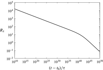
. Figure 1 shows the decay of
 $R_{{\it\lambda}}$
as a function of
 $(t-t_{0})/{\it\tau}$
, where
 $t_{0}=0$
and
 ${\it\tau}=k(0)/\langle {\it\epsilon}(0)\rangle$
when
 $n_{init}=-1.2$
. Notice that there are two distinct (linear) regions corresponding to two practically constant values of
 $n$
;
 $n=n_{init}$
for
 $10^{10}\leqslant (t-t_{0})/{\it\tau}<10^{35}$
and
 $n_{final}$
for
 $(t-t_{0})/{\it\tau}>10^{45}$
. In the initial region (high Reynolds number)
 $R_{{\it\lambda}}$
is expected to be governed by (2.26). Although not predicted by the present SP, the figure seems to suggest that (2.26) is valid in the final period too. Incidentally, figure 1 reveals that
 $R_{{\it\lambda}}$
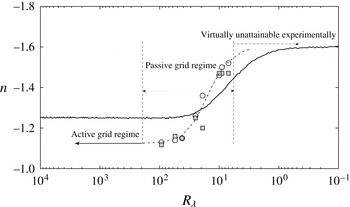
is not constant in the final period of decay and follows a power law. Figure 2, which shows
 $n$
versus
 $R_{{\it\lambda}}$
from figure 1 (the experimental data represented by the symbols will be discussed in § 5), indicates that (2.26) provides reasonable values for
 $n$
, although the initial and final values (
 $-1.25$
and
 $-1.6$
, respectively) differ slightly from the expected ones (
 $-1.2$
and
 $-1.5$
, respectively). It is interesting that the variation of
 $n$
for
 $100\geqslant R_{{\it\lambda}}\geqslant 1$
follows that observed by MS13 (see their figure 11). This is unexpected since (2.26) assumes constant values of
 $n$
. Clearly, (2.26) appears to be valid also when
 $n$
varies, although it is not clear why this is so, and can apparently be used to describe the variation of
 $n$
for the entire decay time.
Variation of
 $R_{{\it\lambda}}$
with time. The MS13 EDQNM data for
 $R_{{\it\lambda}}$
versus
 $(t-t_{0})/{\it\tau}$
were kindly provided by Dr M. Meldi.

Variation of
 $n$
as function of
 $R_{{\it\lambda}}$
according to (2.26), where the approximation
 $R_{l}\equiv R_{{\it\lambda}}$
is used. The solid line corresponds to the data for
 $R_{{\it\lambda}}$
shown in figure 1. The symbols represent the experimental data: circles,
 $n$
is estimated using (4.1); squares,
 $n$
is estimated using (2.26). The dashed-dotted line is used only as a visual guide for the experimental data.

Regardless of the behaviour of
 $c$
with time, the length scale
 $l$
always varies like
 $(t-t_{0})$
. If we identify
 ${\it\lambda}$
with
 $l$
, then plotting
 ${\it\lambda}^{2}{\it\tau}/(t-t_{0})$
as a function of
 $(t-t_{0})/{\it\tau}$
should exhibit a plateau. This is not what we observe in figure 3, although
 ${\it\lambda}^{2}{\it\tau}/(t-t_{0})$
tends towards a constant in the final period of decay, which may suggest that
 ${\it\lambda}$
can be a scaling length in that period. However, MS13 (see figure 7d in MS13) clearly show a lack of collapse for the high-wavenumber region of the ‘
 ${\it\lambda}$
-normalized’ 3D spectra during the final period. Also, the absence of an unambiguous plateau during the initial and transition periods is consistent with the lack of
 ${\it\lambda}$
-scaling of the MS13 spectra (see figure 5d in MS13). While the decrease of
 ${\it\lambda}^{2}{\it\tau}/(t-t_{0})$
in the transition period may reflect the decrease of
 $n$
, the variation in the initial period where
 $n$
is constant is consistent with (2.36). Notice the reduced rate of change in
 ${\it\lambda}^{2}{\it\tau}/(t-t_{0})$
with almost a hint of a plateau before the transition period, suggesting that the turbulence goes through a change of state before entering the transition period.
Variation of
 ${\it\lambda}^{2}{\it\tau}/(t-t_{0})$
with time for the MS13 EQDNM data corresponding to the data of figure 1. The data for
 ${\it\lambda}^{2}{\it\tau}/(t-t_{0})$
versus
 $(t-t_{0})/{\it\tau}$
were kindly provided by Dr M. Meldi.

The variation of
 $n$
from its initial value to its final one over the transition period is likely to be associated with the weakening of the energy transfer
 $\langle ({\rm\Delta}u)^{3}\rangle$
, mainly in the inertial range. In this period, the turbulence is constantly adjusting to the continuous weakening of the transfer of energy as
 $R_{{\it\lambda}}$
decreases and thus cannot reach a self-similar state until the final period, where this transfer is negligible. One may argue that the turbulence state at the end of the transition period acts as an initial condition for the final period.
The results shown in figures 1 and 2 are of significant importance. They show that the initial period is not necessarily associated with
 $n=-1$
. They also illustrate our argument that any value of
 $n\neq -1$
leads to decaying HIT with decreasing Reynolds number at all stages of the decay, while
 $n=-1$
leads to
 $R_{l}$
being constant, regardless of its value. In that context, it is not surprising that using
 $v_{K}$
and
 ${\it\eta}$
as scaling variables leads to
 $n=-1$
, as obtained by Lin (Reference Lin1948) (see also § 4.2) because
 $R_{K}$
is constant (
 $=1$
).
4. Comparison with previous HIT theories of self-preservation
The SP analysis exposed in § 2 was kept as general as possible in order to develop less stringent decay laws than the existing ones. We now look at how the latter can be recovered from our SP analysis, and attempt to explain some apparently conflicting claims from these theories.
4.1. Classical decay laws
The distinguishing feature of the decay laws (2.35a
) and (2.36) relates to the constant of integration,
 $u_{0}^{2}$
. This constant is commonly assumed to be zero, although there is no physical justification for this. If
 $u_{0}^{2}=0$
, we have
 $$\begin{eqnarray}\displaystyle & \displaystyle u^{\prime 2}=-\frac{C_{4}B_{n}}{3C_{3}n}(t-t_{0})^{n}, & \displaystyle\end{eqnarray}$$
 $$\begin{eqnarray}\displaystyle & \displaystyle {\it\lambda}^{2}=-\frac{10{\it\nu}}{n}(t-t_{0}). & \displaystyle\end{eqnarray}$$
 $n$
in the denominator is new. It is common practice to assume that
 $n$
is constant when analysing experimental or numerical data. From a practical point of view, using a power law of the form (4.1a
) with
 $n$
constant and set by the initial conditions, as seen in § 2, is at best an approximation of the decay process over a limited range of
 $t$
, in particular in the transition period where
 $n$
varies with
 $t$
. This certainly explains the various values of
 $n$
reported in the literature. Indeed, most of the measurement and numerical data of decaying HIT are obtained in that period. Clearly, one cannot use (4.1a
) across this period. Rather, one requires a family of power laws of the form
 $(t-t_{0})^{n_{i}}$
, where
 $n_{i}$
is a different constant over each portion
 $i$
of the decay time; this will be illustrated in § 5. Note that regardless of whether or not
 $u_{0}^{2}=0$
,
 $n$
cannot be equal to
 $-1$
. A possible practical alternative to (4.1a
) would be to use a compound power law of the form
 $u^{\prime 2}\sim (t^{(n_{init}+m(t))})$
, where
 $n_{final}-n_{init}\leqslant m(t)\leqslant 0$
.
4.2. Lin’s theory
Lin (Reference Lin1948) used
 $v_{K}$
and
 ${\it\eta}$
as characteristic velocity and length scales in (2.2) and (2.3). After substituting into the KH equation and seeking SP solutions, he obtained
 $$\begin{eqnarray}\displaystyle & v_{K}^{2}=A(t-t_{0})^{-1}, & \displaystyle\end{eqnarray}$$
 $$\begin{eqnarray}\displaystyle & {\it\eta}^{2}=B{\it\nu}(t-t_{0}), & \displaystyle\end{eqnarray}$$
 $$\begin{eqnarray}\displaystyle & \langle {\it\epsilon}\rangle =C(t-t_{0})^{-2}, & \displaystyle\end{eqnarray}$$
 $A$
,
 $B$
and
 $C$
are constants. He then obtained, after integrating expression (4.2c
),
 $$\begin{eqnarray}\displaystyle & u^{\prime 2}={\it\alpha}(t-t_{0})^{-1}+{\it\beta}, & \displaystyle\end{eqnarray}$$
 $$\begin{eqnarray}\displaystyle & {\it\lambda}^{2}=10{\it\nu}(t-t_{0})\{1+({\it\beta}/{\it\alpha})(t-t_{0})\}, & \displaystyle\end{eqnarray}$$
 ${\it\alpha}$
and
 ${\it\beta}$
are constants. These are very similar in form to the present expressions (3.2) and (3.3). However, relations (4.2) are valid on a restricted range of (small) scales only, as illustrated by the collapse of the Kolmogorov normalized spectra or the Kolmogorov normalized second and third structure functions in the dissipative range and, when
 $R_{{\it\lambda}}$
is sufficiently large, the inertial range.
4.3. George’s theory
George (Reference George1992) proposed a theory for decaying HIT based on applying SP to the spectral energy equation. He assumed
 $$\begin{eqnarray}\displaystyle & E(k)=E_{S}\,f_{s}(kl), & \displaystyle\end{eqnarray}$$
 $$\begin{eqnarray}\displaystyle & T(k)=T_{S}g_{s}(kl), & \displaystyle\end{eqnarray}$$
 $E_{S}$
and
 $T_{S}$
, yet to be determined, are unknown functions of time. Clark & Zemach (Reference Clark and Zemach1995, Reference Clark and Zemach1998) also used the SP form
 $E(k)=E_{S}\,f_{s}(kl)$
in their SP analysis based on Lie-group theory. George’s approach differs from the classical approach in that
 $E(k,t)$
and
 $T(k,t)$
are not assumed a priori to scale with single length and velocity scales. In the spatial domain, this is equivalent to (2.2) and (2.3). Further, both analyses lead to (2.22b
) for the scaling length. However, our analysis departs from that of George in a fundamental way. George uses
 $u^{\prime 2}=(2/3)E_{S}l^{-1}\int _{0}^{\infty }f(kl)\,\text{d}k$
to obtain the decay law (4.1). This approach assumes
 $E_{init}(k)=E_{init,SP}(k)$
, implying, in the context of the present analysis, that
 $u_{0}^{2}=0$
and thus yielding
 ${\it\delta}u_{2}\propto u^{\prime 2}$
and
 $l\propto {\it\lambda}$
. Further, George also obtained the expression
 $$\begin{eqnarray}T_{S}=\frac{u^{\prime 3}}{R_{{\it\lambda}}}.\end{eqnarray}$$
This is to be compared to the present formulation
 $$\begin{eqnarray}{\it\delta}u_{3}=c(t){\it\delta}u_{2}^{3/2}=\frac{C_{1}}{\sqrt{\displaystyle \frac{-C_{4}}{3C_{3}n}}}\frac{u^{\prime 3}}{R_{{\it\lambda}}}.\end{eqnarray}$$
To obtain (4.6), we set
 $u_{0}^{2}=0$
in (3.1b
). When
 $n=-1$
,
 $R_{{\it\lambda}}$
is constant and, with the coefficients in (4.6), can be incorporated into the function
 $g$
, thus leading to the classical formulation
 ${\it\delta}u_{3}=u^{\prime 3}$
. If
 $n\neq -1$
but constant then (4.5) and (4.6) are also tenable and
 $c\sim (t-t_{0})^{-(n+1)/2}$
. However, setting
 $l={\it\lambda}$
implies that
 ${\it\delta}u_{2}=u^{\prime 2}$
. Thus, identifying (2.23) with (2.35a
), and (2.24) with (2.35b
) leads, as expected, to
 $u_{0}^{2}=0$
and
 $n=-1$
if
 $c$
is constant (resulting in
 ${\it\delta}u_{3}\sim u^{3}$
), and
 $n=-10/(2C_{3})$
if
 $c\sim (t-t_{0})^{-(n+1)/2}$
(which yields an expression equivalent to (4.5)). Accordingly,
 ${\it\lambda}$
becomes a relevant length scale only when
 $u_{0}^{2}=0$
. Otherwise, it can be an approximate scaling length when (
 $t-t_{0}$
) is small enough for the second term inside the curly brackets of (2.36) to be negligible.
A comment is required regarding (4.5). George (Reference George1992) showed that (4.5) leads to
 $-S_{(\partial u/\partial x)}R_{{\it\lambda}}=\text{constant}$
. We can also reach this result by substituting (2.10) into (2.6) and setting
 $r\rightarrow 0$
since
 $S_{(\partial u/\partial x)}=S_{r=0}$
. This implies that as
 $R_{{\it\lambda}}$
decreases
 $-S_{(\partial u/\partial x)}$
increases indefinitely, which is contrary to experimental and numerical evidence. George (Reference George1992) recognized this inconsistency and proposed that (4.5) is only valid in the initial period where
 $-S_{(\partial u/\partial x)}$
increases until it reaches an upper bound. As stated earlier, the EDQNM results of MS13 do not exhibit such a behaviour. Interestingly, the term
 $C_{1}/(\sqrt{-C_{4}/3C_{3}n+(u_{0}^{2}/{\it\delta}u_{2})})$
in (3.1b
) is consistent with a weakening of
 $\langle ({\rm\Delta}u)^{3}\rangle$
since it decreases while
 $R_{{\it\lambda}}$
decreases during the decay. Finally, George argues that beyond the initial period the turbulence enters another decay regime, which does not necessary comply with SP. It is possible that this is the transition period which leads to the final stage of decay.
5. Comparison with measurements in decaying grid turbulence
Expression (2.26) was tested using the EDQNM data in figure 2, which also reported values of the exponent
 $n$
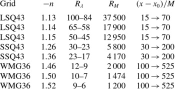
measured downstream of three different grids. Hot-wire measurements were made in our open circuit wind tunnel. The grids consisted of (i) a perforated plate with large square holes and a solidity of 43 % (LSQ43), (ii) a perforated plate with small square holes and a solidity of 43 % (SSQ43) and (iii) an interwoven mesh with a solidity of 36 % (WNG36). Details of the experiments can be found in Kamruzzaman, Djenidi & Antonia (Reference Kamruzzaman, Djenidi and Antonia2013). Table 1 reports the main flow parameters for each grid. The exponent
 $n$
was estimated using two methods. For the first, we assumed a power law of the form (4.1) and used the method of Lavoie, Djenidi & Antonia (Reference Lavoie, Djenidi and Antonia2007) to obtain
 $n$
. In the second method, we used expression (2.26) with the approximation
 $R_{l}=R_{{\it\lambda}}$
to estimate
 $n$
. Remarkably, and despite the expected scatter in the experimental data and the uncertainty associated with each method, both methods yielded approximately the same value of
 $n$
for each grid turbulence. While the experimental data show a similar trend to that of the EDQNM data in the transition period, they differ in magnitude, certainly reflecting the differences in the initial conditions. The relatively good agreement between the experimental results obtained with the power-law method and expression (2.26) confirms that the turbulence in the transition period can be described by a family of power laws, as discussed in § 4.1. Interestingly, most of the measurements in passive grid turbulence fall in the transition period, which can explain the range of values of
 $n$
reported in the literature. On the other hand, one can expect a relatively better agreement among active grid turbulence experiments because the measurements fall in the region of weak variation of
 $n$
with the Reynolds number. Note that this variation becomes smaller, even practically negligible, as
 $R_{{\it\lambda}}$
increases to high values. This will pose a difficult challenge to experimentally detect any
 $R_{{\it\lambda}}$
dependence for
 $n$
. Recently, Sinhuber, Bodenschatz & Bewley (Reference Sinhuber, Bodenschatz and Bewley2015) carried out measurements in passive grid turbulence over a large range of
 $R_{M}$
(
 $1\times 10^{4}\leqslant R_{M}\leqslant 5\times 10^{6}$
,
 $R_{M}$
is the Reynolds number based on the mesh size
 $M$
). They found that
 $n$
is essentially constant (
 $n=-1.18$
) and in agreement with the prediction of Saffman. Unfortunately, the estimate of
 $n$
, whilst obtained with great accuracy, was inferred from the decay of
 $u^{\prime 2}$
over a range of
 $(x-x_{0})/M$
(5–40) which is normally avoided in grid turbulence experiments (Corrsin Reference Corrsin1963) since the flow in this region is not expected to be homogeneous. It is also worthwhile pointing out that the phenomenological approach of Comte-Bellot & Corrsin (Reference Comte-Bellot and Corrsin1966) agrees well with the EDQNM results only at very high and very low
 $R_{{\it\lambda}}$
. The relatively good agreement between the measured values of
 $n$
and those predicted with (2.26) shows that (2.26) is valid outside that range of the Comte-Bellot & Corrsin analysis, i.e. the transition period.
Variations of
 $-n$
,
 $(x-x_{0}/M)$
,
 $R_{{\it\lambda}}$
and
 $R_{M}$
for the (present) experimental data for grid turbulence generated by two perforated plates (LSQ43 and SSQ43) and a woven mesh grid (WMG).

Variation of
 ${\it\lambda}^{2}M/(x-x_{0})$
with
 $(x-x_{0})/M$
in decaying grid turbulence, generated by grid WMG36. Note that for convenience
 $x_{0}=0$
, which does not affect the results.

To test adequately the present laws (2.35)–(2.36), one needs access to the actual scaling velocity and length scales,
 ${\it\delta}u_{2}$
and
 $l$
, respectively, and the constant
 $u_{0}^{2}$
. This is unfortunately not possible. However, one can easily have access to
 ${\it\lambda}^{2}$
, whose variation with respect to time, or in the case of grid turbulence with respect to
 $x$
, can be obtained and compared with (2.36) or (3.3). Note, though, that since the coefficient
 $(u_{0}^{2}/B)$
is expected to be small, a relatively large decay time (or distance behind the grid) may be required for the nonlinear term in (2.36) or (3.3) to become non-negligible. At present, few experimental data at moderately large
 $x/M$
are available, mainly for low-Reynolds-number grid turbulence. Only recently, numerical data on HIT based on the EDQNM simulations have been produced for very long decay times (MS13). On the other hand, the available direct numerical simulation (DNS) data of three-dimensional periodic box turbulence are for a relatively short decay time. Thus, in what follows, we only test the present analysis with the grid turbulence data.
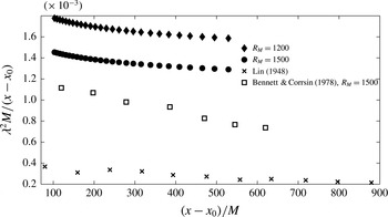
We report in figure 4 the streamwise variations of
 ${\it\lambda}^{2}M/(x-x_{0})$
(for convenience we set
 $x_{0}=0$
, which does not affect the results) in grid turbulence generated by the grid WMG36. The data should show a plateau if
 ${\it\lambda}^{2}$
follows (4.1b
) with
 $n$
constant. The figure also includes the data of Bennett & Corrsin (Reference Bennett and Corrsin1978) and Lin (Reference Lin1948). Clearly, none of the curves has a plateau, implying that
 ${\it\lambda}^{2}$
does not vary like
 $(x-x_{0})$
. Arguably, the variation of
 $n$
over the distance
 $0\leqslant (x-x_{0})/M\leqslant 900$
may induce a curvature in the data. However, we believe that this is not the case since the variation of
 $R_{{\it\lambda}}$
with
 $x/M$
is too small to produce a significant difference in
 $n$
. Another possibility that explains the curvature is the influence of the nonlinear term in (2.36) or (3.3). This term becomes important when
 $(t-t_{0})$
(or
 $(x-x_{0})$
) becomes large. For small values of
 $(t-t_{0})$
, the first term in the curly brackets of (2.36) dominates and
 ${\it\lambda}$
varies like
 $(t-t_{0})$
(assuming
 $n$
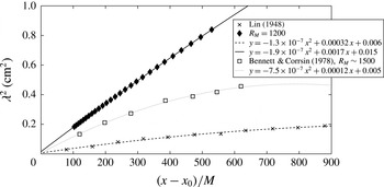
is constant). To investigate this influence, a quadratic fit has been applied to all the data sets of figure 4, and is shown in figure 5. It is important to remember that because
 $n<-1$
for the data in figure 5, using a quadratic form (i.e.
 $n=-1$
) to represent the data is strictly not correct and some caution should be exercised when interpreting the results of figure 5 (the data for
 $R_{M}=1500$
are not shown for clarity). Nevertheless, the quadratic fit provides an indication of the effect of the nonlinear term. Interestingly, all the data appear to be well represented by this fit, highlighting the relatively important effect of the nonlinear term in (2.36); changing the exponent
 $n$
from
 $-1$
to
 $-1.2$
, for example, will only accentuate this effect. Also, the small negative value of the coefficient of the second-order term of the fit is consistent with the prediction
 $u_{0}^{2}\leqslant 0$
made earlier. Although this coefficient is likely to vary with
 $n$
, it remains negative.
Quadratic fit to
 ${\it\lambda}^{2}$
in decaying grid turbulence.

The magnitude of the coefficient of the linear term should not be affected by the nonlinear term. According to (3.3), this coefficient should be equal to
 $10{\it\nu}M/(U_{0})$
, which for
 $R_{M}=1200$
is about 0.0021. This is about 23 % larger than the value (0.0017) obtained from the quadratic fit. Based on the information provided in Bennett & Corrsin (Reference Bennett and Corrsin1978), we estimate
 $10{\it\nu}M/U_{0}=0.001$
for their data, which is relatively close to the coefficient shown in the figure. Unfortunately, there is insufficient information to estimate the coefficient for the fit to Lin’s data. When
 $n<-1$
, the coefficient should be
 $-10{\it\nu}M/(U_{0}n)$
(see (2.36)). Kamruzzaman et al. (Reference Kamruzzaman, Djenidi and Antonia2013) assumed a power-law decay of the form (4.1) and measured
 $n=-1.5$
for the data at
 $R_{M}=1200$
. This value of
 $n$
leads to a coefficient about 17 % smaller than 0.0017.
6. Conclusions
A self-preservation (SP) analysis has been applied to the transport equation of the velocity structure function,
 $\langle ({\rm\Delta}u)^{2}\rangle$
, in decaying HIT, with the view to establishing a general framework of SP which can be used to appraise existing SP analyses and test SP solutions both numerically and experimentally. The present SP formulation follows a similar approach to that of Barenblatt & Gavrilov (Reference Barenblatt and Gavrilov1974); it does not a priori assume a single velocity scale for both
 $\langle ({\rm\Delta}u)^{2}\rangle$
and
 $\langle ({\rm\Delta}u)^{3}\rangle$
. However, the analysis departs from all previous analyses in that it introduces the skewness
 $S$
of the longitudinal velocity increment, which can be expressed as
 $S=c(t){\it\phi}(r^{\ast })$
, where
 $c$
and
 ${\it\phi}$
are dimensionless functions of time and
 $r^{\ast }$
, respectively. SP can be achieved when
 $c(t)$
is constant or varies like
 $(t-t_{0})^{-(n+1)/2}$
as the turbulence decays. It is shown that when
 $c$
is constant,
 $n=-1$
and the Kolmogorov length (
 ${\it\eta}$
) and velocity (
 $v_{K}$
) scales are ‘natural’ scaling variables. On the other hand, the Taylor microscale,
 ${\it\lambda}$
, does not play any particular role in the present SP analysis, and the scaling velocity cannot in general be identified with
 $u^{\prime }$
, the r.m.s. velocity fluctuation. However, when
 $c\sim (t-t_{0})^{-(n+1)/2}$
,
 ${\it\lambda}$
can be a relevant scaling length when
 $(t-t_{0})$
is small.
The decay laws for the turbulent kinetic energy
 $k$
and the Taylor microscale
 ${\it\lambda}$
which ensue from the present analysis can be regarded as a generalization of existing decay laws, such as those of Lin (Reference Lin1948), Barenblatt & Gavrilov (Reference Barenblatt and Gavrilov1974) and George (Reference George1992). For example, when SP holds, the kinetic energy decays as
 $k\sim (t-t_{0})^{n}+B$
, where
 $B$
is a constant. It is argued that
 $B$
represents the energy of the motions whose scales are excluded from the SP range of scales at the initial time. Thus, when
 $B=0$
, SP is achieved at all scales of motion and
 ${\it\lambda}$
becomes a relevant scaling length together with the Kolmogorov length scale.
The analysis not only confirms the dependence of
 $n$
on the initial conditions, but shows how this dependence is related to the initial length and velocity scales. Further, when the initial condition is such that
 $n=-1$
,
 $R_{{\it\lambda}}$
can have any value but must remain constant throughout the decay; any other value of
 $n({<}-1)$
induces a decaying turbulence with
 $R_{{\it\lambda}}$
decreasing with time.
Acknowledgements
The financial support of the Australian Research Council is gratefully acknowledged. The authors also thank Dr M. Meldi for providing the EDQNM data and Mr Md Kamruzzaman for carrying out the grid turbulence measurements.