Introduction
Our knowledge of the internal structure of the Earth and of the source parameters of large earthquakes is largely based on records provided by worldwide seismological observatories. Unfortunately, the coverage of the Southern Hemisphere by seismic stations is significantly lower than that of the Northern Hemisphere. Despite an effort to improve the southern high latitude coverage that started during the 1957–58 International Polar Year, large southernmost regions remain under-sampled. This is ascribable to the prevalence of oceans in these regions, to the high microseismic noise around latitude 50°S caused primarily by the oceans, and also to the logistical constraints involved in setting up stations on the Antarctic continent. In the early 1990s, there were only nine permanent broadband stations in Antarctica, of which only one (South Pole) was located in the interior of the continent.
Setting up new seismological stations in central Antarctica is of major interest for a number of scientific studies related to the Earth structure from subsurface to deep interior, and to the evolution and dynamics of the continent itself. Many technical difficulties have to be solved, due to the very low temperatures, to the inaccessibility of the region, to the necessity of generating electrical power without generating vibrations in a region in which the sun disappears for months at a time, and due to the need to set up seismometers in stable conditions on ice. Even when these difficulties are overcome, the data themselves exhibit specific features that require particular processing because the presence of a thick ice sheet modifies the seismic signal compared to the signal recorded on rock. A good understanding of the signal induced by the ice sheet, and an appropriate correction of this perturbation, are essential before exploiting these data using standard techniques.
In this paper, we report on the analysis of the seismic ice-signal at the Dome C site in central East Antarctica, where a new permanent observatory (the second one on the ice cap in the interior of the continent) has been set up in the past decade (Lévêque et al. unpublished). More recently, three temporary stations have also been installed at the site (Maggi & Lévêque in press). We present results obtained using the horizontal to vertical (H/V) spectral ratio approach, a method usually implemented to evaluate soil response in seismic regions for seismic risk evaluation, but which, to our knowledge, has never been used to infer the ice cap response.
Seismological experiments at Dome C
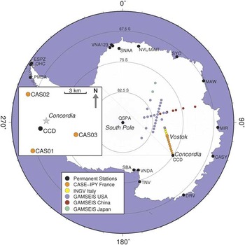
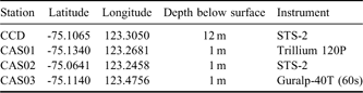
Since 1998 École et Observatoire des Sciences de la Terre (EOST) in Strasbourg and Istituto Nazionale di Geofisica e Vulcanologia (INGV) in Rome, in collaboration with their national polar agencies Institut Paul Emile Victor (IPEV) and Programma Nazionale Richerche in Antartide (PNRA), have set up a permanent seismological observatory at the French-Italian scientific base Concordia (CCD), under the “Seismology at Concordia” research programme (Fig. 1). The station (code CCD, Table I) is located at Dome C at about 1000 km from the coast of Terre Adélie and at about 1 km from Concordia base. It was constructed progressively over six summer campaigns, at the same time as the scientific base itself. The two STS-2 seismometers at CCD have been recording continuously since the start of full time occupation of the scientific base (December 2004), in a seismic vault whose temperature is a constant -54°C (the yearly average temperature at Dome C). One of the scientific results we expect from this station is an improvement of regional and global images of the Earth interior.
Map of Antarctica with the permanent seismic stations, and the seismic profiles planed in the frame of POLENET for the 2007–08 International Polar Year. Box: Location of the CCD station and of the three temporary stations at Dome C near the French-Italian base Concordia.

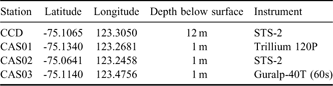
Coordinates of the four seismic stations at Concordia considered in this study. Site elevation is 3240 m.
The “Seismology at Concordia” programme also calls for the deployment of an antenna of autonomous and isolated seismic stations, in order to escape human-related noise and to increase sensitivity to small amplitude seismic phases thanks to specific antenna-related techniques (Fig. 1). Such an antenna would facilitate, for example, the observation of seismic waves that cross the inner core along polar paths, which are crucial for constraining inner core anisotropy and differential rotation, and thus for better understanding internal Earth dynamics (Souriau Reference Souriau1998, Reference Souriau2007). This part of the seismic programme at Concordia requires solving problems caused by the external temperature (-30°C in summer, -70°C in winter) and the four months per year of darkness, which make it particularly difficult to ensure an autonomous non-vibrating energy source. Technical solutions to these difficulties have recently become available, as attested by the success of the Transantarctic Mountains Seismic Experiment (TAMSEIS) project (Lawrence et al. Reference Lawrence, Wiens, Nyblade, Anandakrishnan, Shore and Voigt2006).
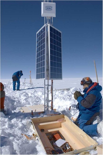
In preparation for the 2007–08 International Polar Year, Polar Earth Observing Network (POLENET) experiment (http://classic.ipy.org/development/eoi/proposal-details.php?id=185, accessed February 2009; http://www.institut-polaire.fr/api/la_recherche_francaise_et_l_api/185_polar_earth_observing_network, accessed February 2009), we developed and constructed three prototype autonomous stations, which we deployed at 1 m depth on a circle of ∼5 km radius around CCD during the summer of 2007–08 (Fig. 1). Each of these stations (CAS01, CAS02, CAS03) is powered by three 85 W solar panels and ten 60 Ah gel-acid batteries (Fig. 2). The stations are designed to hibernate during the winter months, with the large number of batteries ensuring three to four weeks autonomy during the Antarctic night. The stations are equipped with three different seismometers, as shown in Table I. The lessons learned from this test deployment were integrated in the construction of the autonomous stations deployed for the French segment of the POLENET experiment. In this study we analysed data from CCD and from the three prototype autonomous stations.
Set-up of the autonomous seismological broadband station CAS03 inside the Antarctic continent, 5 km away from Dome C.

The seismic and mechanical properties of ice
The ice cap at Dome C has mostly been investigated for palaeoclimatic purposes, important parameters being accumulation rate with time and ice dynamics related to ice rheology and internal stress field (Durand et al. Reference Durand, Gillet-Chaulet, Svensson, Galiardini, Kipfstuhl, Meyssonnier, Parrenin, Duval and Dahl-Jensen2007). The total thickness of the ice cap at Dome C is ∼3270 m. Its fine structure is mostly known from airborne radar, which detects changes in the dielectric properties of ice (Tabacco et al. Reference Tabacco, Passerini, Corbelli and Gorman1998), and from a deep core that sampled the entire ice column (EPICA community 2004). Radar data have revealed that the internal layers of the ice at the location of CCD are sub-horizontal down to at least 2000 m depth. Three internal layers have been traced continuously in the uppermost 2000 m on the basis of the dielectric properties, and have been related to isochronous deposits during the last 100 000 years (Siegert et al. Reference Siegert, Eyers and Tabaco2001). The pattern of the earlier (deeper) isochronous layers is more complex. Chemical analyses of the ice core permitted the identification of eight glacial cycles during the last 740 000 years (EPICA community 2004). The presence of nearby subglacial lakes has also been detected from radio-echo sounding (Siegert et al. Reference Siegert, Carter, Tabacco, Popov and Blankenship2005).
The mechanical properties of the polar cap are related to the size of the grains, to the preferred orientation of crystals, and to the presence of pores and bubbles. The ice crystals are in hexagonal compact form with a strong intrinsic anisotropy (Gagnon et al. Reference Gagnon, Kiefte, Clouter and Whalley1988). During ice deformation due to snow accumulation and increase in pressure, crystals rearrange with a preferred orientation so that the c-axes are aligned in the vertical direction, generating seismic anisotropy with P-wave velocities about 15–20% higher in the vertical direction than in the horizontal directions. The elastic parameters of ice as determined on ice glaciers (Press Reference Press1966, Gagnon et al. Reference Gagnon, Kiefte, Clouter and Whalley1988) are as follows: P-wave velocity increases from 3.6–3.8 km s-1 at 0°C to ∼3.9–4.0 km s-1 at -16°C, S-wave velocity increases from 1.6–1.7 km s-1 to ∼2.0 km s-1 at the same temperatures, and the Poisson’s ratio is high, of the order of 0.30–0.33.
The density ρ is a crucial parameter for characterizing the evolution from snow to ice (Paterson Reference Paterson1994). ρ = 0.55 g cm-3 corresponds to the transition from a discontinuous arrangement of the spheres to a packed arrangement in a continuous, dense rhombohedral lattice. This transition is likely to induce a sharp increase in S-wave velocity. ρ = 0.73 g cm-3 corresponds to the state of maximum contact between grains, and ρ = 0.84 g cm-3 corresponds to the complete closure of the pores, the remaining air being present as bubbles (Paterson Reference Paterson1994). In Concordia, the depths corresponding to these densities are about 23, 65 and 100 m respectively, then the density increases slowly with depth up to 0.92 g cm-3 at 3000 m at the base of the ice column (Duval, personal communication 2009, Arnaud, personal communication 2010, Brunjail et al. unpublished data). Unfortunately, no seismological prospecting devoted to the knowledge of the ice sheet has been performed at Dome C. Seismic results from experiments on glaciers (e.g. Gagnon et al. Reference Gagnon, Kiefte, Clouter and Whalley1988, Jarvis & King Reference Jarvis and King1995) and on Erebus ice shelf (http://www.anta.canterbury.ac.nz/documents/2008-09%20projects%20GCAS/Armstrong.pdf, accessed February 2009) will be used as initial constraints of our models.
The horizontal to vertical spectral ratio method
The H/V method is commonly used to determine soil response to a seismic excitation for seismic risk evaluation (e.g. Field & Jacob Reference Field and Jacob1995). It consists of computing the ratio between the horizontal and vertical components either on S-waves and S-coda of local earthquakes (Lermo & Chavez-Garcia Reference Lermo and Chavez-Garcia1993), or on noise records (Nakamura Reference Nakamura1989, Bard Reference Bard1999). This method is often applied in urban environments, where noise is permanently produced by anthropogenic activity. For a station installed on rock with little topography, the H/V ratio is close to unity (Bard Reference Bard1999). In sedimentary basins, H/V values of up to 10 or more may be observed at some frequencies (Borcherdt Reference Borcherdt1970, Lebrun et al. Reference Lebrun, Hatzfeld and Bard2001, Souriau et al. Reference Souriau, Roullé and Ponsolles2007). If a soft, sedimentary layer of thickness h is present over a rocky half space, a resonance peak with fundamental frequency f = vS/4h is observed, where vS is the S-wave velocity inside the layer. This simple relationship is no longer valid if the impedance contrast between surficial layers and substratum is weak (Malischewsky & Scherbaum Reference Malischewsky and Scherbaum2004), if several layers are present, or if there is significant topography. If the structure is complex, the peak frequencies and amplitudes are difficult to interpret on their own (http://sesame-fp5.obs.ujf-grenoble.fr/Delivrables/Del-D23-HV_User_Guidelines.pdf, accessed January 2010), and synthetic seismograms may be useful to model the observations.
If the structure is unknown, the H/V noise spectrum may provide constraints on the structure of the uppermost layers. It gives information on the S-wave velocity, which is the most interesting parameter from the mechanical point of view, because it is very sensitive to the lack of continuity of the medium and to the presence of fluid inclusions (bubbles or partial melting). At Dome C, it may give information on the structure of the ice cap, as S-wave velocity contrasts are expected inside the ice layer and at its base. This method requires only a few tens of minutes of seismic record from a single three component instrument, it does not require natural earthquakes or active sources, and it is thus easy to implement. In addition, it gives information on the nature of the ambient noise. Unfortunately, a strong drawback of this method is the non-uniqueness of the models fitting the spectra, so that external information is generally required to help constrain the models.
From a general point of view, seismic noise includes natural microseisms due primarily to the oceans, and microtremors due to anthropogenic activity. Microseisms are Rayleigh waves caused by the interaction of ocean waves with the solid earth (e.g. Friedrich et al. Reference Friedrich, Krüger and Klinge1998), they have characteristic periods between four and ten seconds, depending on the location on Earth. Noise of anthropogenic origin is more complex and appears predominantly at periods T<1 s. It includes body waves (P and S) and surface waves (Rayleigh and Love) generated by traffic, industrial and domestic activity and the interaction of wind with buildings. The relative contribution of the different types of waves (body waves, fundamental and higher modes of surface waves) to the noise exhibits significant variability (see the review by Bonnefoy-Claudet et al. Reference Bonnefoy-Claudet, Cotton and Bard2006). The human activity at Dome C is important enough to generate a significant domestic noise. At the temporary stations, on the other hand, the noise will be dominated by microseismic noise and wind-ground interaction.
Results
We have analysed data from the four seismic stations at Dome C: the permanent observatory CCD and three autonomous stations CAS01, CAS02 and CAS03. The instrument bandpass and the relatively low sampling rate (0.05 s) impose strong limitations on analysing the high frequency side of the H/V spectral ratio, which will be cut at 10 Hz. At each site, we have analysed noise at four different epochs. For each epoch, 20 noise records of 25.6 s length (512 points) have been selected. The spectra are computed for each of the three components of motion in the frequency range 0.05–10 Hz using a Fast Fourier Transform, and smoothed on windows 1/6 decade wide in order to remove instabilities without removing the resonance peaks. We merge the two horizontal components E (east–west) and N (north–south) according to H = (E2 + N2)1/2 to account for the partition of the noise energy on the two components. The mean and standard deviation of the spectra are obtained by processing twenty independent noise windows.
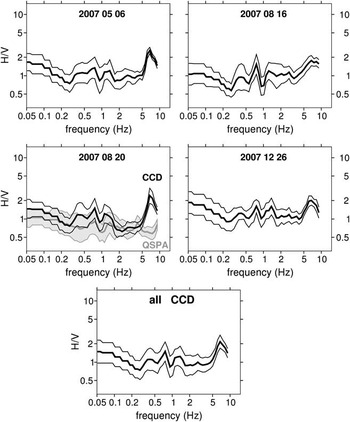
Figure 3 shows H/V ratios at CCD for the four epochs considered. We observe similar features in the spectra, despite some variability even for days that are close in time (e.g. 16 August 2007 and 20 August 2007). The peak amplitudes are weak (H/V < 3) compared to values commonly obtained for sedimentary basins. The most prominent peak is observed at high frequency (6.7 Hz), three weaker peaks are observed at 0.40, 0.75 and 1.30 Hz. In classical urban environments, these peaks would be considered as only marginally significant because of their low amplitude. However, as the same resonance frequencies are observed in all the spectra from each station, they may be more significant in the particular Antarctic context, and indicative of the structure beneath the stations. In particular, the resonance at high frequency suggests an origin related to the structure of the ice sheet.
H/V spectral ratios determined from noise at site CCD at four different epochs, and mean spectral ratio for the site. Each curve is reported with its 1σ confidence level. For comparison is reported (in grey) the H/V spectral ratio for an instrument at 275 m depth in a borehole at station QSPA near South Pole, for 20 August 2007.

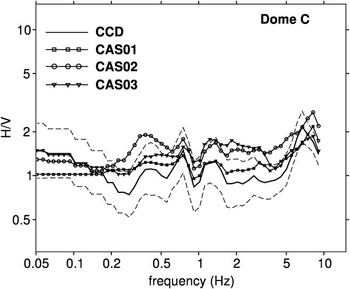
Similar results are obtained at the autonomous stations (Fig. 4), with a slightly higher frequency for the main peak (∼8 Hz), suggesting a resonance in a slightly thinner layer, or slightly higher velocities in the ice sheet. For these stations, we also observe a higher mean H/V level, which is probably due to the poorer installation conditions, resulting in a stronger influence of the wind on the horizontal components.
Mean H/V spectral ratios determined from noise at the four Dome C stations. The 1 σ confidence level is nearly the same for the different curves, it is given for CCD only (dashed line).

For comparison, Fig. 3 shows the H/V ratio obtained at the QSPA station located five miles away from the Amundsen–Scott Base at the South Pole. The QSPA instrument we have used for this analysis is installed in a borehole at 275 m depth. The total ice sheet thickness at South Pole is about 2.5 km. We have chosen to analyse data from 20 August 2007 because of the strong high-frequency content of the noise during this day, which permits a clear identification of the high frequency peak at 6.7 Hz at CCD. This resonance peak is not present at QSPA, whereas the peaks at 0.75 and 1.3 Hz are well observed at both stations. The absence of the peak at 6.7 Hz at QSPA suggests that it is generated by the uppermost snow layer. On the other hand, we note that the very low frequency signal is reduced at QSPA compared to CCD, probably because of the reduced influence of wind on buried instruments.
Discussion
One dimensional modelling with synthetic seismograms
A resonance frequency is observed when there is a strong vertical elastic impedance contrast. This may occur at the transition between snow and firn or firn and ice, when the ice crystals are compacted so that they become strongly interconnected. Following Lachet & Bard (Reference Lachet and Bard1994) and Souriau et al. (Reference Souriau, Roullé and Ponsolles2007), we have modelled seismic noise via the summation of synthetic seismograms. This method is applied here because it allows us to vary noise composition, compared to most other methods which assume that noise is predominantly composed of Rayleigh waves (e.g. Stephenson et al. Reference Stephenson, Hartzell, Frankel, Asten, Carver and Kim2009). In particular, using our method, we may include both surface waves and body waves, and introduce shear sources for generating Love waves, which may represent a significant contribution to noise (Bonnefoy-Claudet et al. Reference Bonnefoy-Claudet, Cotton and Bard2006).
We generate synthetic noise by summing 1000 synthetic seismograms whose specific parameters (distance, type of source, form of far field, frequency, amplification and delay) are defined randomly in pre-defined ranges (Souriau et al. Reference Souriau, Roullé and Ponsolles2007). For a given structure, each elementary seismogram is generated using the reflectivity method (Müller Reference Müller1985). The sources are randomly distributed around the site at distances between 100 and 500 m. Sources are explosions, single vertical forces, and shear sources with three possible far-field forms: a single pulse, a single oscillation, or a three-arch oscillation. The dominant period ranges from 0.03 to 0.5 s, with a logarithmic distribution in order to generate more high frequencies than low frequencies as is typical for domestic noise. The summation of the 1000 seismograms is done after randomly assigning an amplification and a time delay to each of them.
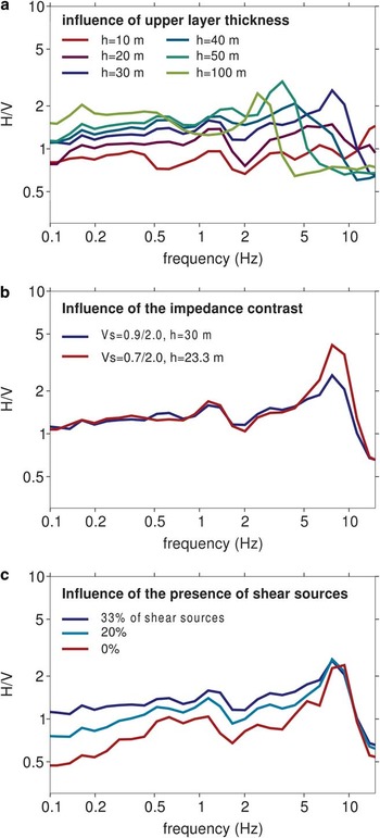
Figure 5a shows how the thickness of the unconsolidated snow layer influences the H/V spectrum, for thicknesses varying between 10 and 100 m, and for an S-wave velocity of 0.9 km s-1 in this layer and 2.0 km s-1 in the solid ice (all the other parameters remain unchanged). The resonance frequency shifts toward lower values when the thickness of the soft layer increases, and is close to the theoretical value expected for a one layer model, f = vS/4h. Figure 5b shows the drastic influence of the impedance contrast at the base of the soft layer on the peak amplitude. When the S-wave velocity in the upper layer is decreased from 0.9 to 0.7 km s-1 (thus an increase of the impedance contrast close to 1.1), the peak amplitude increases by a factor close to two. For an easier comparison of the spectra, the thickness of the upper layer has been decreased from 30 to 23 m, so that the peak position remains unchanged (according to f = vS/4h, there is a trade-off between the S-wave velocity and the thickness in the resonant layer). Finally, as shown in a previous study (Souriau et al. Reference Souriau, Roullé and Ponsolles2007), the composition of the noise influences the H/V spectra, in particular the presence of shear sources. In Fig. 5a & b, the noise was composed of an equal proportion of explosions, single vertical forces and shear sources. Figure 5c compares the results with 33, 20 and 0% of shear sources, the other types of sources being in equal proportion. The presence of shear sources does not perturb the peak position, but it significantly increases the H/V ratio at low frequency.
Modelling of the H/V spectral ratio from synthetic seismograms. a. Influence of the thickness of the snow layer (note the shift in frequency of the resonance peak). b. Influence of the impedance contrast at the base of the snow layer. c. Influence of the composition of the noise.

Given the reports of subglacial lakes in the region surrounding Dome C (Siegert et al. Reference Siegert, Carter, Tabacco, Popov and Blankenship2005), we have also tested the influence of a thin (5 m thick) liquid layer at the base of the ice column. It turns out that it has no detectable effect on the synthetic H/V spectral ratio in the frequency range considered.
Comparison with observations
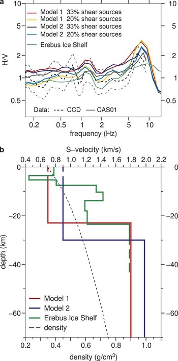
In Fig. 6a, the H/V observations at CCD and CAS01 are superimposed on the H/V spectra obtained from synthetic seismogram modelling for two models and two noise compositions. Model 1 (preferred, Fig. 6b) introduces a sharp velocity contrast at 23 m depth, where a continuous ice lattice appears. This model correctly explains the peaks at 7.5 and 1.3 Hz. The mean velocity in the firn above this layer is low (0.7 m s-1). For comparison we show the velocity profile for the Erebus ice shelf at Ross Island, deduced from surface wave analysis (http://www.anta.canterbury.ac.nz/documents/2008-09%20projects%20GCAS/Armstrong.pdf, accessed February 2009). In this model, a sharp discontinuity is observed at the same depth (23 m), but the uppermost velocities are significantly higher, as milder thermal conditions favour snow compaction. The very low uppermost velocities at Dome C are a consequence of the low compaction rate due to the extremely low temperatures, which prevent melting at any time of the year, so that compaction is mostly governed by pressure and sublimation (Paterson Reference Paterson1994). Note that the Erebus ice shelf model is unable to reproduce the H/V peak at 7.5 Hz, confirming the need for low uppermost velocities in the Dome C model. There is, however, a large range of possible models. To illustrate the non-uniqueness of the solution, we show the results for a model with the same sharp velocity contrast located at 30 m depth (model 2, Fig. 6b). The fit of the data is comparable to that obtained with model 1 (Fig. 6a).
a. Fit of the H/V spectral ratios at the Dome C stations CCD (dashed, with standard deviation) and at CAS01 (grey line), with two different models and two different compositions of the noise. Also shown is the result obtained for the Erebus ice shelf model, with different climatic conditions (http://www.anta.canterbury.ac.nz/documents/2008-09%20projects%20GCAS/Armstrong.pdf, accessed February 2009). b. S-wave velocity models used in a. (scale at the top, model 1 preferred), and density profile at Concordia (L. Arnaud, personal communication 2010, scale at the bottom).

We have not been able to explain the small peak at 0.75 Hz, even with the introduction of other impedance contrasts at greater depth. This peak is also present at QSPA, thus it is probably related to a change in seismic properties with depth. A discontinuity at 300 m depth can explain the peak, but with unrealistically low velocities (Asten, personal communication 2010). At the temporary stations, the peak at 8 Hz may be explained by a slightly thinner soft layer (22 m), or by slightly higher velocities in the firn layer (0.75 m s-1), or both, as varying conditions of compactions are suggested by the great variability of density in the uppermost 15 m (Arnaud, personal communication 2010). Finally, the dielectric discontinuities identified from radar measurements (Siegert et al. Reference Siegert, Eyers and Tabaco2001) do not appear as seismic discontinuities, even in the uppermost 2000 m where the H/V method has a good resolution.
Results relative to the noise composition at Dome C are also obtained from our modelling. As illustrated in Fig. 5c, noise composition mostly influences the low frequency spectrum. A spectrum without shear sources explains correctly the high frequency peak. This result is not surprising if we consider the moderate domestic activity at Concordia, and the low quality factor for shear waves in firn, which prevents efficient propagation of shear signals from the base to the station, about 1 km away. By contrast, a significant contribution of shear noise (with 20–30% of shear sources) is required to fit the low frequency side of the spectra. This low frequency shear noise is probably induced by the presence of wind and its coupling with the surface. The lower H/V low frequency signal at the QSPA borehole instrument also favours this interpretation.
Conclusion and perspectives
Only two permanent seismic observatories are set up on the ice cap inside the Antarctic continent. It is thus of interest to analyse the specific response of these stations to seismic excitation. Thanks to the analysis of the H/V spectral ratio of the ambient noise, we have been able to specify the seismic properties of the uppermost, unconsolidated snow layer at Dome C, and its seismic contrast with the solid ice. The preferred model, which includes a 23 m layer with S-wave velocity of 0.7 km s-1 overlying a layer with S-wave velocity of 1.8 km s-1, explains the main features of the spectra. This sharp S-wave velocity contrast coincides in depth with a density of 0.55 g cm-3, and is identified as the transition to a compact arrangement of ice spheres in a continuous lattice. We have also been able to detect a small geographic variability of the unconsolidated layer in a 5 km region around Concordia. The simpler spectrum obtained at the South Pole station QSPA at 275 m depth corroborates the idea that the high frequency peak at CCD is generated by the uppermost snow layer, and shows the interest of installing the instruments in boreholes, when possible. We have not been able to detect the discontinuities revealed by radar methods, indicating that dielectric and seismic properties appear to be uncorrelated.
The model given by the H/V method is non-unique, due in particular to a trade-off between layer thicknesses and S-wave velocities. However, this method, which is easy to implement, is a valuable tool to investigate the uppermost structure of the ice cap and its lateral variation, in the absence of other information. The results of a complementary approach, based on the retrieval of the ice transfer function from records of remote earthquakes, will be discussed elsewhere. The knowledge of this transfer function is crucial in order to correct the seismic signal for the influence of the ice cap, so that the signal can be analysed using routine procedures for earthquake source parameter determination and Earth structure computations. Specific seismic experiments devoted to the seismic imaging of the ice cap would be useful to determine the P- and S-wave velocity profiles and the seismic anisotropy in the ice beneath Concordia.
Acknowledgements
Funding and logistical support for the seismology programme at Concordia is provided by IPEV and PNRA. The French contribution to POLENET is funded by ANR (Agence Nationale de la Recherche) via the CASE-IPY project (Concordia, Antarctica, Seismic Experiment for the International Polar Year). The observatory station CCD is run in collaboration with our colleagues at INGV: Stefania Danesi, Andrea Morelli, Alberto Delladio. We thank Jacques Burdin, Jean-Yves Thoré and Maxime Bès de Berc for their invaluable contribution to the design and installation of CCD and the autonomous CASE stations. We also thank all the summer and winter personnel at Concordia base for helping us install and run the stations. Thanks also to Paul Duval, from the “Laboratoire de Glaciologie” at Grenoble for useful information about ice properties at Dome C, to Loïc Jahan for computing facilities, to M. Asten and two other anonymous reviewers for useful comments, and to C. Hulbe for her editorial work.