Introduction
Direction-of-arrival (DOA) estimation in an antenna array system has been an intensive research area in communications, radar, and many other fields [Reference Godara1] for several decades. Various techniques have been proposed for estimating DOA of far-field, narrowband sources, including the traditional subspace methods and recently developed sparse methods. The MUltiple SIgnal Classification (MUSIC) algorithms [Reference Swindlehurst and Kailath2, Reference Osman, Sfar and Gharsallah3] and the Estimation of Signal Parameters via Rotational Invariance Techniques (ESPRIT) [Reference Roy and Kailath4, Reference Zoltowski, Haardt and Mathews5] are undoubtedly the most successful super-resolution methods, which are based on the orthogonality of subspaces. However, these subspace-based methods are sensitive to coherent sources. Thus, some methods [Reference Ma, Dong and Xie6, Reference Vikas and Vakula7] are proposed to solve the source correlation by spatial smoothing technique without considering gain-phase errors. With the recent advances in sparse signal processing [Reference Candes and Wakin8, Reference Carlin, Rocca, Oliveri, Viani and Massa9], the performance of DOA estimation algorithms have been further enhanced by exploiting the spatial sparsity in direction of sources. The sparse methods estimate DOAs by applying sparse representation and compressed sensing techniques. In particular, the continuous direction range is approximated by a set of discrete grid points and the DOAs are assumed to lie on a prescribed grid. Those sparse methods are so popular in recent decades due to these obvious pro: no prior knowledge of the number of sources, small number of snapshots (even a single snapshot), and robustness to coherent sources. The available sparse algorithms are mainly divided into three categories [Reference Yang, Li, Stoica and Xie10]: on-grid algorithms [Reference Stoica, Babu and Li11, Reference Stoica and Babu12], off-grid algorithms [Reference Cui, Duan and Liu13, Reference Yang, Xie and Zhang14], and gridless algorithms [Reference Yang, Xie and Zhang15, Reference Yang and Xie16]. The on-grid methods are also dependent on the grid selection so that they inevitably encounter the problem of grid mismatch. The off-grid and gridless methods are applied to cope with the grid mismatch problem. Moreover, the gridless methods completely solve it because of direct operating in the continuous domain. The semiparametric iterative covariance-based estimation (SPICE) method [Reference Stoica, Babu and Li11] uses the covariance fitting criteria which have sound statistical motivation. The source power and noise variances are estimated by alternate iteration. In [Reference Yang, Xie and Zhang15], the sparse and parametric approach (SPA) is a discretization-free sparse method, which is also based on covariance fitting criteria, and first ever introduced for continuous DOA estimation which completely eliminates grid mismatches in existing grid-based methods. In addition, the SPICE + pp method is also advanced to further improve the performance of both the SPICE and the SPA.
Although those subspace and sparse methods have excellent performance of DOA estimate, they are critically dependent on the knowledge of array manifold. Unfortunately, in practical application scenarios, the array manifold is often influenced by unknown gain-phase errors. Without array manifold calibration, the estimator's performance could degrade substantially [Reference Zhou and Wen17]. Therefore, it is necessary to develop DOA estimation methods in the presence of array errors. The existing correction methods are mainly divided into two categories [Reference Lemma, Deprettere and van der Veen18]: active calibration methods and self-calibration methods. The active calibration method [Reference Peng, Gao, Qu and Guo19] performs offline estimation of the array error parameters by setting the precisely known calibration signals, which is rarely guaranteed in practice. An improved offline method [Reference Dai, Su, Gu and Li20] is proposed by using two calibration sources in unknown direction, but it is also invalid when directions of the two calibration sources are equal. The self-calibration methods are carried out online and are blind approaches. They can estimate the perturbation as well as DOA of sources simultaneously and do not require knowledge of the exact locations of sources. The method in [Reference Weiss and Friedlander21], named as the WF method for convenience, is based on alternative iteration algorithm for simultaneously estimating the DOA and gain-phase errors. However, it requires the assumption that the array perturbations are small. The error estimation in [Reference Li and Er22] is facilitated by considering the Toeplitz structure of the sample covariance matrix without calibration signals, however, it is limited to the array with particular geometries. The method in [Reference Liao and Chan23] uses the ESPRIT technique to estimate the DOA and gain-phase errors, but requires the information of calibrated sensors. Other methods in [Reference Liu, Liao, Zeng, Yang and Xu24, Reference Hu and Xu25] present non-iterative algorithms which have the advantage that DOA estimates are independent of gain-phase errors, but require two signals spatially far separated from each other. All of them [Reference Weiss and Friedlander21–Reference Hu and Xu25] do not consider the gain-phase errors in the case of coherent signals. Coherent signals usually exist in some scenarios, such as wireless communication systems, which result in rank deficiency of the sample data covariance matrix, and the above-mentioned methods may not be application. To the best of our knowledge, however, there are very limited methods that can resolve DOAs of coherent signals in the presence of unknown gain-phase errors.
Considering these issues, in this paper, a new iteration method is proposed to estimate the DOA of uncorrelated and coherent signals with gain-phase errors simultaneously. First, the gain errors are estimated by using the diagonal of the covariance matrix subtracting the noise term. Second, inspired by the SPICE method, the source power and noise variances in the case of existing gain-phase errors are deduced respectively because gain-phase errors just have effects on the signal sources. Finally, we estimate the phase errors by introducing an exchange matrix and combining the WF method. The exchange matrix is a special case of forward and backward space smoothing method and can reduce the correlation between signal sources. Furthermore, the proposed method is applied to solve the problem of performance degradation in the SPA method under the condition of gain-phase errors. The problem is addressed by using the estimated gain-phase errors and source powers of the proposed method as initial values of the SPA with gain-phase errors, which is called the combined method.
Compared with the available works, our method has two contributions: (1) estimate the DOA and gain-phase errors simultaneously for not only the uncorrelated sources but also the coherent sources. (2) Resolve the problem of performance deterioration of the SPA method with gain-phase errors. Some experiments are performed on the varying gain error ranges, varying signal to noise ratios (SNRs) and varying snapshots, and the simulation results verify that the proposed method has well performance of estimating DOA and gain-phase errors in the uncorrelated sources and the coherent sources cases, and illustrate that the combined method can improve the performance of the SPA in the case of gain-phase errors.
Notations used in this paper are as follows. Throughout the paper, we use capital italic bold letters to represent matrices and operators, and lowercase italic bold letters to represent vectors. For a given matrix  ${\bi A}$,
 ${\bar {\bi A}}$ denotes the complex conjugate matrix,
 ${\bi A}^{\bi T}$ denotes the transpose,
 ${\bi A}^{\bi H}$ represents the conjugate transpose matrix, and A mn denotes the
 $(m, n)$ the element of
 ${\bi A}$.
 $tr({\bi A})$ denotes the trace of
 ${\bf A}$. I denotes the identity matrix.
 $\left\Vert \cdot \right\Vert$ denotes the Frobenius norm for matrices and l 2 norm for vectors.
 ${\hat {\bi R}}$ is an estimator of R and E[ • ] denotes expectation.
The rest of the paper is organized as follows. In the Section “Data model”, the mathematical model is formulated. In the Section “The proposed method”, the calibration algorithm is presented. Section “A combined method” introduces a combined method. Section “numerical Simulations” presents simulation results. Conclusions are drawn in the Section “Conclusion’.”
Data Model
Consider a linear array of M isotropic sensors radiated by D narrowband far-field sources. Let θ = [θ 1, …, θ K]T and  $\lcub {\theta_k} \rcub _{k = 1}^K $ denotes a grid that covers Ω ∈ [ − 90°, 90°). Ω denotes the set of possible locations, and K denotes the grid number. For simplicity we assume that the signal sources and the sensors are coplanar, take the first sensor as the reference point, and fix its location as the origin of coordinates, i.e., (x 1, y 1) = (0, 0). The elements are uniformly distributed on the x axis, and the array spacing is half-wavelength. The observed signals at the uniform linear array (ULA) along the x axis are given by
 $${\bi y}(t) = \sum\limits_{k = 1}^K {{\bi a}(\theta _k)s_k(t)} + {\bi n}(t) = {\bi A}({\bi \theta} ){\bi s}(t) + {\bi n}(t)\quad t = 1,\, \ldots, \,N(M \times 1)$$
where y(t), s(t), and n(t) denote the observed snapshot, the vector of source signals, and the vector of measurement noise, respectively.  ${\bi a}(\theta _k) = [1\;{\rm e}^{j\pi \,\sin \,\theta _k} \ldots \;{\rm e}^{j(M - 1)\pi \,\sin \,\theta _k}]^T$ is the steering vector. t denotes the
 $t {\rm th}$ snapshot. M is the number of sensors and N is the snapshot number. A(θ) is the array manifold matrix given by A(θ) = [a(θ 1),…, a(θ K)].
Equation (1) denotes the ideal model without gain-phase errors. Considering the gain-phase errors, (1) should be rewritten as
 $${\bi y}(t) = {\bi \Gamma A}({\bi \theta} ){\bi s}(t) + {\bi n}(t) = {\bi G\Phi A}({\bi \theta} ){\bi s}(t) + {\bi n}(t)$$
where  ${\bi \Gamma = G\Phi} = {\rm diag}([\alpha _1e^{{\rm -} j\phi _1},\, \ldots, \,\alpha _Me^{{\rm -} j\phi _M}]^T)$ denotes the gain-phase errors. G = diag([α 1, …, α M]T) and α m denotes the gain-error diagonal matrix and the gain error of the mth sensor.
 ${\bi \Phi} = {\rm diag}([e^{ - j\phi _1},\, \ldots, \,e^{ - j\phi _M}]^T)$ and ϕ m denotes the phase-error diagonal matrix and the phase error of the mth sensor. α 1 = 1, ϕ 1 = 0.
More compactly, (2) can be written as
 $${\bi Y} = {\bi \Gamma A}({\bi \theta} ){\bi S} + {\bi E}$$
where
 $$\eqalign{& {\bi Y} = [{\bi y}(1),\, \ldots, \,{\bi y}(N)] \cr & {\bi S} = [{\bi s}(1),\, \ldots, \,{\bi s}(N)] \cr & {\bi E} = [{\bi n}(1),\, \ldots, \,{\bi n}(N)]} $$
Assumption 1: The noise n(t) is assumed to be spatially and temporarily uncorrelated.
 $$E[{\bi n}(t_1){\bi n}^H(t_2)] = {\rm diag}({\bi \sigma} )\delta _{t_1,t_2}$$
where σ = [σ 1, …, σ M]T denotes the noise variance and  $\delta _{t_1,t_2}$ is a delta function.
 $$\delta _{t_1,t_2} = \left\{ {\matrix{ {1,} & {{\rm if}\,t_1 = t_2} \cr {0,} & {{\rm elsewhere}} \cr}} \right.$$
Assumption 2: The source signals s(t) is independent of the noise n(t).
 $$E[{\bi s}(t_1){\bi s}^H(t_2)] = {\rm diag}({\bi p})\delta _{t_1,t_2}$$
where p = [p 1, …, p K]T denotes the source power.
Assumption 3: The data snapshots {y(1), …, y(N)}(n!/(r!(n − r)!) are uncorrelated with each other and have the following covariance matrix:
 $$\eqalign{{\bi R} &= E[{\bi y}(t){\bi y}_{}^H (t)] \cr &= {\bi \Gamma A}({\bi \theta }){\rm diag}({\bi p}){\bi A}^H({\bi \theta }){\bi \Gamma }^H + {\rm diag}({\bi \sigma }) \cr &= [{\bi \Gamma }{\bi a}_1, \ldots ,\,{\bi \Gamma }{\bi a}_K ]\left[ {\matrix{ {\,p_1} & 0 & \cdots & 0 \cr 0 & \ddots & \cdots & \vdots \cr \vdots & \vdots & \ddots & \vdots \cr 0 & \cdots & \cdots & {\,p_K} \cr } } \right]\left[ {\matrix{ {{\bi a}_1^H {\bi \Gamma }^H} \cr \vdots \cr {{\bi a}_K^H {\bi \Gamma }^H} \cr } } \right] \cr& {\rm + }\left[ {\matrix{ {\sigma _1} & 0 & \cdots & 0 \cr 0 & \ddots & \cdots & \vdots \cr \vdots & \vdots & \ddots & \vdots \cr 0 & \cdots & \cdots & {\sigma _M} \cr } } \right] \cr &= [{\bi \Gamma }{\bi a}_1, \ldots ,\,{\bi \Gamma }{\bi a}_K {\bi I}]\left[ {\matrix{ {\,p_1} & 0 & \cdots & \cdots & \cdots & \cdots & 0 \cr 0 & {\,p_2} & 0 & \cdots & \cdots & \cdots & 0 \cr \vdots & 0 & \ddots & \vdots & \vdots & \vdots & \vdots \cr 0 & \cdots & \cdots & {\,p_K} & \cdots & \cdots & 0 \cr 0 & \cdots & \cdots & \cdots & {\sigma _1} & \cdots & 0 \cr \vdots & \vdots & \vdots & \vdots & \vdots & \ddots & \vdots \cr 0 & \cdots & \cdots & \cdots & \cdots & \cdots & {\sigma _M} \cr } } \right] \cr&\left[ {\matrix{ {{\bi a}_1^H {\bi \Gamma }^H} \cr \vdots \cr {{\bi a}_K^H {\bi \Gamma }^H} \cr {\bi I} \cr } } \right]} $$
The Proposed Method
Gain error estimation
Denote  ${\hat {\bi R}} = {\bi Y}{\bi Y}^H/N$ as the sample covariance. The eigendecomposition of
 ${\hat {\bi R}}$ is given as
 $${\hat {\bi R}}{\rm =} \sum\limits_{m = 1}^M {\gamma _{{\hat {\bi R}}, m}} {\bi u}_{{\hat {\bi R}}, m}{\bi u}_{{\hat {\bi R}}, m}^H $$
where  $\lcub {\gamma_{{\hat {\bi R}}, m}} \rcub _{m = 1}^M $ denotes the eigenvalues and
 $\lcub {{\bi u}_{ {\hat {\bi R}}, m}} \rcub _{m = 1}^M $ is the corresponding eigenvectors. Arrange those eigenvalues in descending order. Correspondingly,
 $\lcub {\gamma_{ {\hat {\bi R}}, m}} \rcub _{m = 1}^D $ are the signal eigenvalues and
 $\lcub {\gamma_{{\hat {\bi R}},m}} \rcub _{m = D + 1}^M $ are the noise eigenvalues.
Therefore the average value of  $\lcub {\sigma {}_m} \rcub _{m = 1}^M $ can be given as
 $$\bar \sigma = \sum {\lcub {\gamma_{{\hat {\bi R}},\,m}} \rcub _{m = D + 1}^M} /M - D$$
Define R(m, m) as the main diagonal of R, the gain errors can be estimated as
 $$\hat \alpha _m = {\rm sqrt}\left( {\displaystyle{{R(m,m) - \bar \sigma} \over {R(1,1) - \bar \sigma}}} \right)\quad m = 1,\, \ldots, \,M$$
DOA estimation with gain-phase errors
We consider the following covariance fitting criterion for the purpose of parameter estimation when N ≥ M:
 $$g({\bi \theta },{\bi p,\sigma ,\Gamma }) = \vert \vert {{\bi R}^{{{ - 1} / 2}}({\hat {\bi R}} - {\bi R}){{\hat {\bi R}}}^{{{ - 1} / 2}}} \vert \vert^2$$
where R−1/2 denotes the square root of R−1, and both  ${\hat {\bi R}}$ and R are invertible.
We need to calculate P and σ separately, rather than using a uniform formula in SPICE method, because the amplitude and phase errors only affect P.
A simple calculation shows that
 $$\eqalign{g &= {\rm tr}[{\bi R}^{ - 1/2}({\hat {\bi R}} - {\bi R}){{\hat {\bi R}}}^{ - 1}({\hat {\bi R}} - {\bi R}){\bi R}^{ - 1/2}] \cr &= {\rm tr}({\bi R}^{ - 1}{\hat {\bi R}}) + {\rm tr}({{\hat {\bi R}}}^{ - 1}{\bi R}) - 2M \cr & = {\rm tr}({{\hat {\bi R}}}^{1/2}{\bi R}^{ - 1}{{\hat {\bi R}}}^{1/2}) + \sum\limits_{k = 1}^K {({\bi a}_k^H {\bi \Gamma }^H{{\hat {\bi R}}}^{ - 1}{\bi \Gamma }{\bi a}_k)p_k} \cr &+ \sum\limits_{k = K + 1}^{K + M} {{{\hat {\bi R}}}^{ - 1}\sigma _{k - K}} - 2M} $$
The problem of minimizing g can be written as the following constrained minimization:
 $$\fleqalign{\mathop {{\rm min}}\limits_{\lcub {\,p_k \ge 0,\sigma_k \ge 0} \rcub } {\rm tr}({\hat {\bi R}}^{1/2}{\bi R}^{ - 1}{\hat {\bi R}}^{1/2})\;{\rm s}{\rm. t}{\rm.} \;\sum\limits_{k = 1}^K {w_kp_k +} \sum\limits_{k = K + 1}^{K + M} {w_k\sigma _{k - K}} = 1$$
where
 $$w_k = \left\{ {\matrix{ {{\bi a}_k^H {\bi \Gamma}^H{{\hat {\bi R}}}^{ - 1}{\bi \Gamma} {\bi a}_k/M} & {k = 1,\, \ldots, \,K} \cr {{{\hat {\bi R}}}^{ - 1}/M} & {k = K + 1,\, \ldots, \,K + M} \cr}} \right.$$
We introduce  ${\bi C =} \lsqb {{\bi c}_1^H, \, \ldots, \,{\bi c}_{K + M}^H} \rsqb \in {\opf C}^{\lpar {K + M} \rpar \times M}$ and have that (readers are referred to [Reference Stoica, Babu and Li11] for the detailed procedure)
 $$\eqalign{{\bi C}^H{\bi P}^{ - 1}{\bi C} \ge & {\bi C}_0^H {\bi P}^{ - 1}{\bi C}_0 \cr &= {{\hat {\bi R}}}^{1/2}{\bi R}^{ - 1}{{\hat {\bi R}}}^{1/2}\;{\rm s}{\rm. t}{\rm.} \;{\bi A}^H{\bi C =} {{\hat {\bi R}}}^{1/2}} $$
where  ${\bi C}_0 = {\bi PA}{\bi R}^{ - 1}{\hat {\bi R}}^{1/2}$ is the solution (for fixed P) of the problem
 $$\mathop {{\rm min}}\limits_{\bi C} {\rm tr}({\bi C}^H{\bi P}^{ - 1}{\bi C})\;{\rm s}{\rm .t}{\rm .}\;{\bi A}^H{\bi C = }\;{\hat {\bi R}}^{1/2}$$
It is easy to obtain that
 $${\rm tr}({\bi C}^H{\bi P}^{ - 1}{\bi C}) = {\rm tr}({\bi P}^{ - 1}{\bi C}{\bi C}^H) = \sum\limits_{k = 1}^K {\displaystyle{{{\left\Vert {{\bi c}_k} \right\Vert}^2} \over {\,p_k}}} + \sum\limits_{k = K + 1}^{K + M} {\displaystyle{{{\left\Vert {{\bi c}_k} \right\Vert}^2} \over {\sigma _{k - K}}}} $$
Combining (13) and (15), this function (17) is to be minimized with respect to {p k ≥ 0, σ k−K ≥ 0}, subject to
 $$\sum\limits_{k = 1}^K {w_kp_k +} \sum\limits_{k = K + 1}^{K + M} {w_k\sigma _{k - K}} = 1$$
By the Cauchy–Schwarz inequality
 $$\eqalign{&\left[ {\sum\limits_{k = 1}^K {w_k^{{1 / 2}} \left\Vert {{\bi c}_k} \right\vert} + \sum\limits_{k = K + 1}^{K + M} {w_k^{{1 / 2}} \left\Vert {{\bi c}_k} \right\Vert} } \right]^2 \cr & \quad \le \left[ {\sum\limits_{k = 1}^K {\displaystyle{{{\left\Vert {{\bi c}_k} \right\Vert}^2} \over {\,p_k}}} + \sum\limits_{k = K + 1}^{K + M} {\displaystyle{{{\left\Vert {{\bi c}_k} \right\Vert}^2} \over {\sigma _{k - K}}}} } \right]\left[ {\sum\limits_{k = 1}^K {w_kp_k + } \sum\limits_{k = K + 1}^{K + M} {w_k\sigma _{k - K}} } \right] \cr & \quad = \sum\limits_{k = 1}^K {\displaystyle{{{\left\Vert {{\bi c}_k} \right\Vert}^2} \over {\,p_k}}} + \sum\limits_{k = K + 1}^{K + M} {\displaystyle{{{\left\Vert {{\bi c}_k} \right\Vert}^2} \over {\sigma _{k - K}}}} }$$
Therefore the solution to (19) is
 $$p_k = \displaystyle{{\left\Vert {{\bi c}_k} \right\Vert} \over {w_k^{{1 / 2}} \rho}}, \quad k = 1,\, \ldots, \,K$$
 $$\sigma _{k - K} = \displaystyle{{\left\Vert {{\bi c}_k} \right\Vert} \over {w_k^{{1 / 2}} \rho}}, \quad k = K + 1,\, \ldots, \,K + M$$
 $$\rho = \sum\limits_{m = 1}^{K + M} {w_m^{{1 / 2}} \left\Vert {{\bi c}_m} \right\Vert} $$
C0 is as the first step and substituted into (20–22) above, and we have the updating formulas
 $$P_k^{i + 1} = P_k^i \displaystyle{{\left\Vert {{\bi a}_k^H {{\rm (}{\bi \Gamma} ^i{\rm )}}^H{{\rm (}{\bi R}^i)}^{ - 1}{{\hat {\bi R}}}^{1/2}} \right\Vert} \over {w_k^{1/2} \rho ^i}}\quad k = 1,\, \ldots, \,K$$
 $$\sigma _{k - K}^{i + 1} = \sigma _{k{\rm -} K}^i \displaystyle{{\left\Vert {{({\bi R}^i)}^{ - 1}{{\hat {\bi R}}}^{1/2}} \right\Vert} \over {w_k^{1/2} \rho ^i}}\;\quad k = K + 1, \ldots, K + M$$
 $$\rho ^i = \sum\limits_{m = 1}^K {w_m^{1/2} p_m^i} \left\Vert {{\bi a}_m^H {({\bi \Gamma} ^i)}^H{({\bi R}^i)}^{ - 1}{{\hat {\bi R}}}^{1/2}} \right\Vert + \sum\limits_{m = K + 1}^{K + M} {w_m^{1/2} \sigma _{m{\rm -} K}^i} \left\Vert {{({\bi R}^i)}^{ - 1}{{\hat {\bi R}}}^{1/2}} \right\Vert $$
In the case of identical  $\lcub {\sigma_k^{}} \rcub $, it is the special case of (24) and (25), and is easy to obtain that
 $$\sigma ^{i + 1} = \sigma _{}^i \displaystyle{{\left\Vert {{({\bi R}^i)}^{ - 1}{{\hat {\bi R}}}^{1/2}} \right\Vert} \over {\left( {{\sum\nolimits_{k = K + 1}^{K + M} {w_k^{}}}^{1/2}\rho^i} \right)}}$$
 $$\rho ^i = \sum\limits_{m = 1}^K {w_m^{1/2} p_m^i} \left\Vert {{\bi a}_m^H {({\bi \Gamma} ^i)}^H{({\bi R}^i)}^{ - 1}{{\hat {\bi R}}}^{1/2}} \right\Vert + \sigma _{}^i \sum\limits_{m = K + 1}^{K + M} {w_m^{1/2}} \left\Vert {{({\bi R}^i)}^{ - 1}{{\hat {\bi R}}}^{1/2}} \right\Vert $$
Phase-error estimation
In this section, we introduce an exchange matrix to reduce the correlation between signal sources without affecting the estimated performance in the case of unrelated sources. JM is an M-order exchange matrix, in which the counter-diagonal elements are 1 and the remaining elements are all 0. JMJM = IM.
Denote  ${\bi x}(t) = {\bi J}_M {\bar {\bi y}}(t)$, the covariance matrix of x(t) is
 $${\bi R}_{\bi x} = E[{\bi x}(t){\bi x}_{}^H (t)] = {\bi J}_M {\bar {\bi R}}{\bi J}_M$$
Let  ${\bi R}_1 = {\bi R +} {\bi R}_{\bi x} = {\bi R} + {\bi J}_M {\bar {\bi R}}{\bi J}_M.$ The noise subspace V = [VD+1, VD+2, …, VD+M] can be obtained by the characteristic decomposition of
 $${\bi R}_1 \; {\bar {\bi y}}\lpar t \rpar $ and
 ${\bar {\bi R}}$ are the complex conjugate matrix of y(t) and R, respectively.
For ith iteration, we can get a new generation pi, and find the D highest peaks of the estimated power variance, and the corresponding DOAs  $\lcub {\theta_k^i} \rcub _{k = 1}^D $ from this iteration, where pi and θi are arranged in descending order.
Denote φ = [ϕ 1, …, ϕ M]T, and the updating iteration of phase errors can be estimated as
 $${\bi \varphi} ^i = - {\rm angle}({\bi z}^i)$$
 $${\bi z}^i = \displaystyle{{{({\bi Q}^i)}^{ - 1}{\bi h}} \over {{\bi h}^T{({\bi Q}^i)}^{ - 1}{\bi h}}} {\bi h} = [1,0, \ldots, 0]^T$$
 $${\bi Q}^i = \sum\limits_{k = 1}^D {{[{\rm diag}({\bi a}(\theta _k^i ))]}^H{\bi VV}_{}^H {\rm diag}({\bi a}(\theta _k^i ))} $$
where angle( • ) denotes the phase of a complex number.
Compute Γi from the estimated gain errors G and phase errors φi:
 $${\bi \Gamma} ^i = {\rm diag}([\alpha _1, \ldots, \alpha _M]^T){\rm diag}(\exp ( - j{\bi \varphi} ^i))$$
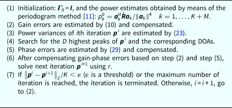
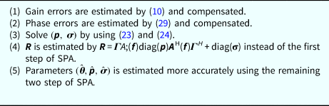
Consequently, the proposed method is summarized as follows.
A Combined Method
In order to estimate the DOAs of arriving sources without discretizing the spatial angles, we transform the angular parameters to the frequency ones.
Denote
 $$f_d = (\sin \lpar {\theta_d} \rpar + 1)/2 \in [0,1),\;d \in [D]$$
where f = [f 1, …, f D]T is called the frequency parameter, and the relation θ ↔ f is one-to-one. Therefore, the new steering matrix can be written as A(f) = [a(f 1),…, a(f D)], with  ${\bi a}(f_d){\rm =} [1,{e^{i2\pi f_d}, \ldots, e^{i2(M - 1)\pi f_d}]^T,\quad d = 1, \ldots, D.$ According to the SPA method, the minimization of (12) is equivalent to
 $$\eqalign{& \mathop {\min} \limits_{{\bi X},{\bi \Gamma}, {\bi u},\lcub {{\bi \sigma} \underline{ \succ} 0} \rcub } {\rm tr}({\bi X}) + {\rm tr}({\bi \Gamma} ^H{{\hat {\bi R}}}^{ - 1}{\bi \Gamma} T({\bi u})) + {\mathop{\rm Re}\nolimits} ({\rm diag}({{\hat {\bi R}}}^{ - 1})^H){\bi \sigma} \cr & {\rm subject\ to}\; \left[ {\matrix{ {\bi X} & {{{\hat {\bi R}}}^{\textstyle{1 \over 2}}} & {} \cr {{{\hat {\bi R}}}^{\textstyle{1 \over 2}}} & {{\bi \Gamma} T({\bi u}){\bi \Gamma}^H{\rm +} {\bi \sigma}} & {} \cr {} & {} & {T({\bi u})} \cr}} \right] \ge 0} $$
where T(u) = A(f)diag(p)AH(f) is a (Hermitian) Toeplitz matrix which is determined by its first row u.
Equation (34) cannot be solved by the semidefinite programming (SDP) convex tools in the SPA to obtain R. In order to cope with this problem, we improve the SPA method by replacing the first step of the SPA method with the estimated parameters of the proposed method, called the combined method.
Numerical Simulations
In this section, we illustrate the performance of proposed methods through simulations. The range of the DOAs of signals is confined in [ − 90°, 90°]. The gain errors  $\lcub {\alpha_m} \rcub _{m = 1}^M $ and phase errors
 $\lcub {\phi_m} \rcub _{m = 1}^M $ of the sensors are generated by
 $$\alpha _m = 1 + \sqrt {12} \sigma _\alpha \zeta _m$$
 $$\phi _m = \sqrt {12} \sigma _\phi \eta _m$$
where ζ m and η m are independent and identically distributed random variable distributed uniformly over [ − 0.5, 0.5].σ α and σ ϕ are the standard deviations of α m and ϕ m, respectively. In the simulations below, σ α = 0.1.
Effect of signal sources correlation
In our simulation, we consider D = 3 sources with power p = [3, 3, 5]T from directions θ = [10°, 25°, 60°]T. A ULA with M = 10 is used to receive the signals. Let the sample number N = 200 and the grid number K = 180 for SPICE+ (‘ +’ indicates the condition that the noise variances are equal in this paper). The SNR is 30 dB.
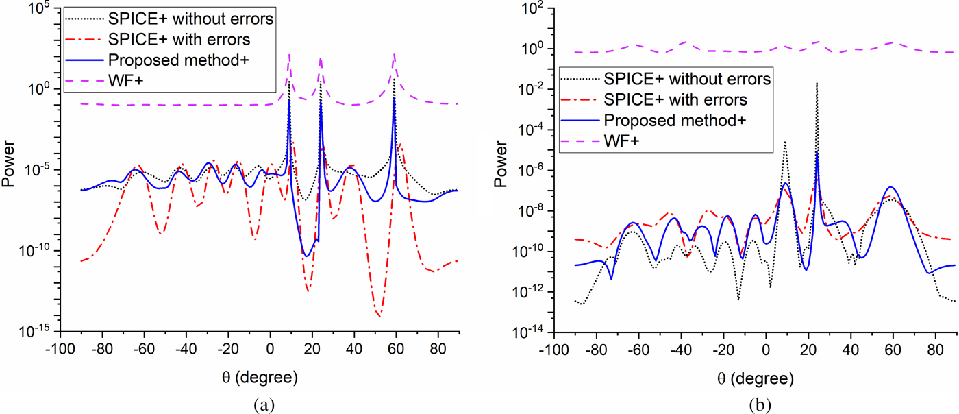
It can be seen from Fig. 1(a) that in the case of uncorrelated sources, the performance of the SPICE with gain-phase errors is severely deteriorated. But after calibrating the gain and phase errors by the proposed method in Table 1, the spatial spectrum can clearly form sharp peaks at three incident directions. Obviously, the method proposed in [Reference Weiss and Friedlander21] (in the following we refer to it as the WF method) can also correct the errors well under this condition. However, the WF method almost completely fail in the correlated sources case (Fig. 1(b)). In contrast, the proposed algorithm can form effective peaks at three directions of arrival. Therefore, the calibration algorithm proposed in this paper has successfully corrected the gain and phase uncertainties for the uncorrelated sources and the coherent sources.
Spectra of SPICE+ without gain-phase errors, SPICE+ with gain-phase errors, the proposed method+ and WF+ in the case of uncorrelated sources and coherent sources. (a) Sources are uncorrelated, and σ ϕ = 40° and (b) sources are coherent (source3 is a replica of source1) and σ ϕ = 15°.

The proposed algorithm.

Effect of sample number
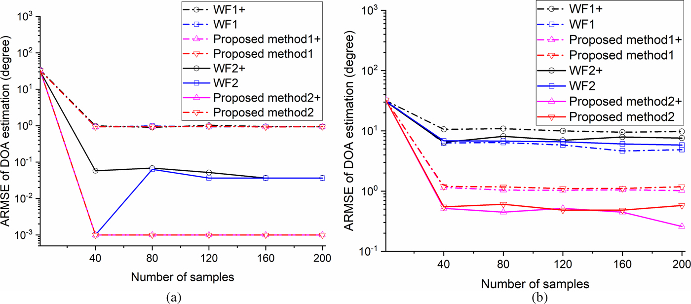
Consider three signals with the power p = [3, 3, 5]T from θ = [10°, 25°, 60°]T. The SNR is 20 dB and the sample number is 200. Based on 500 Monte Carlo runs, the average root mean square error (ARMSE) of DOA versus the number of samples with uncorrelated sources and coherent sources are shown in Figs 2(a) and 2(b), respectively.
ARMSE of DOA estimation versus the number of samples (a) sources are uncorrelated (the dashed and solid plots represent the cases of σ ϕ = 20° and σ ϕ = 5°, respectively) and (b) sources are coherent (the dashed and solid plots represent the cases of σ ϕ = 15° and σ ϕ = 5°, respectively).

Figure 2(a) plots that the four curves almost coincide in the case of large phase errors, but the proposed method outperforms the WF method when the phase errors are small. Figure 2(b) presents that the proposed method performs better than the WF method in the coherent sources case as the snapshot number increases. In addition, regardless the number of samples, the proposed method is better when noise variances are equal.
Effect of phase errors
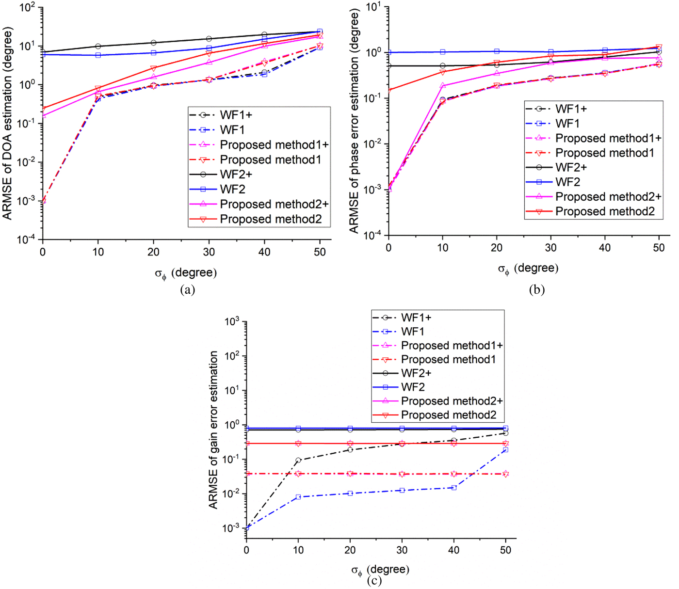
Consider three signals impinging on the ULA array from directions 10, 25 and 60°, respectively. Based on 500 Monte Carlo runs, the ARMSE of DOA, phase error and gain error estimates versus the standard deviation of the phase error σ ϕ are obtained by the WF method and the proposed method, respectively. We show the results in two different experiment conditions: uncorrelated sources and coherent sources.
From Figs 3(a) and 3(b), it is shown that both the proposed method and the WF method perform well in the uncorrelated sources case for DOA and phase error estimates. In contrast, it is illustrated that the proposed method behaves better than the WF method when the sources are coherent. It is because the covariance fitting criteria is robust to the coherent sources and the exchange matrix of the new method reduces the correlation of sources. In addition, they fall into suboptimal solutions in large phase error. On the other hand, Fig. 3(c) presents the gain error estimation of the proposed method is stable and performs better because it is independent of the phase errors.
(a) ARMSE of DOA estimation versus σ ϕ, (b) ARMSE of phase error estimation versus σ ϕ and (c) ARMSE of gain error estimation versus σ ϕ (the dashed and solid plots represent the cases of uncorrelated signal sources and coherent signal sources, respectively).

Effect of SNR
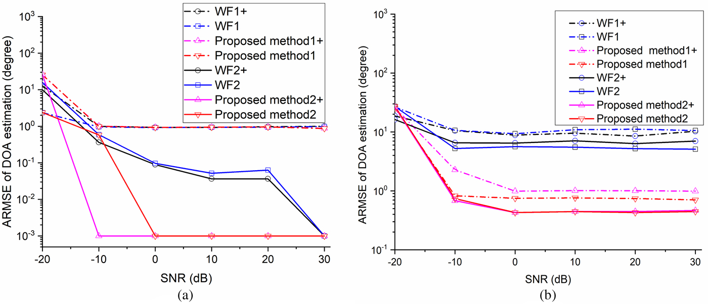
We repeat the simulation by fixing sample number N = 200 and varying SNR from −20 to 30 dB. 500 Monte Carlo runs are used for the performance of the aforementioned methods versus the SNR, where the sources signals are in two cases.
Figure 4(a) presents that both the proposed method and the WF method have similar performance trends as the SNR increases and perform well in the case of large phase errors. However, the proposed method performs better in the case of small phase errors. From Fig. 4(b), it is shown that when signal sources are coherent, the WF method fails during all varying SNR. To the contrary, the curve of the proposed method is constantly slower than that of the WF method.
ARMSE of DOA estimation versus the SNR (a) sources are uncorrelated (the dashed and solid plots represent the cases of σ ϕ = 20° and σ ϕ = 5°, respectively) and (b) sources are coherent (the dashed and solid plots represent the cases of σ ϕ = 15° and σ ϕ = 5°, respectively).

Application on SPA method with gain-phase errors
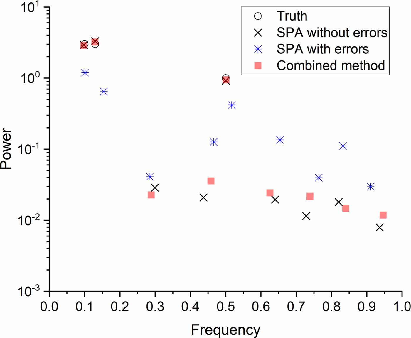
In this subsection, we consider three uncorrelated sources with power p = [3, 3, 1]T from directions by the frequency vector f = [0.10, 0.13, 0.50]T. A ULA with M = 10 is considered. The SNR is 30 dB and sample number is 200. σ ϕ = 30°.
From Fig. 5, it is illustrated that the performance of SPA degrades substantially when the gain and phase errors exist. After calibration by the combined method in Table 2, the estimated points almost coincide with the truth points.
Spectra of SPA without gain-phase errors, SPA with gain-phase errors and the combined method for uncorrelated sources.

The combined algorithm.

Conclusion
In this paper, the DOA estimation problem in the presence of gain-phase errors is addressed. The proposed method in Table 1 does not require the presence of calibration sources and previous calibration information. Moreover it performs well not only in the case of uncorrelated sources during a large phase error range but also in the case of coherent sources in the small and moderate phase error range. Meanwhile, combining the proposed method and the SPA method in Table 2 solves the problem of deteriorate performance of the SPA with gain-phase errors. The main drawback is converging to suboptimal solution in large phase errors. However, it is worth mentioning that the AMRSE of DOA estimated by the proposed method is about 1° when σ ϕ = 30°(corresponding phase error range is [−51.96° 51.96°]) in uncorrelated sources case and σ ϕ = 15° (corresponding phase error range is [−25.98° 25.98°]) in coherent sources case (Fig. 3), respectively. Therefore, the proposed method is effective in practical application scenarios.
Author ORCIDs
Wencan Peng 0000-0002-1592-667X
Acknowledgments
This work was supported by the National Natural Science Foundation of China (Nos. 61771380, U1730109, and 61771376) and the Foundation of the State Key Laboratory of CEMEE (No. 2017K0202B).
 Wencan Peng was born in Hubei Province, China, in 1987. She received her B.S. degree from the School of Measuring and Optical Engineering, Nanchang Hangkong University in Nanchang city, China, in 2010. Then, she received her M.S. degree from the School of Electronics and Information, Northwestern Polytechnical University in Xi'an city, China, in 2013. Now, She is pursuing her Ph.D. degree at the School of Electronics and Information, Northwestern Polytechnical University. Her research interests include array signal processing and array calibration.
 Chenjiang Guo was born in Shaanxi Province, China, in 1963. He is a CIE Senior Member and an Antenna Society Committee Member. He received his B.S., M.S., and Ph.D. from the School of Electronics and Information, Northwestern Polytechnical University in Xi'an city, China, in 1984, 1987, and 2007, respectively. He is a professor at the School of Electronics and Information NWPU. He has published more than 140 research papers. His research interests include array signal processing and theory and design of antenna.
 Min Wang (IEEE Member) received his B.S. degree from Xidian University, China in 2000; his M.S. and Ph.D. degrees in Signal and Information Processing from Xidian University, Xi'an, China, in 2003 and 2005, respectively. He is working at National Lab of Radar Signal Processing in Xidian University. His research interests include sparse signal processing, milliwave/Terahertz radar, and high-resolution radar imaging.
 Yuteng Gao was born in Shaanxi Province, China, in 1988. He received his B.S. and M.S. degrees from the School of Electronics and Information, Northwestern Polytechnical University in Xi'an city, China, in 2010 and 2013, respectively. He is presently pursuing his Ph.D. degree in the School of Electronics and Information, Northwestern Polytechnical University in Xi'an city, China. His research interests include millimeter wave, antenna design, and radar imaging.