1 Introduction
The liquid/solid/gas contact line (CL) marks the boundary between wet and unwet support. A liquid advances along a support by displacing the surrounding gas. Alternatively, if the liquid retreats it may unwet the previously wet support, in which case gas replaces liquid. For CLs moving at high enough speeds,
 $U_{CL}$
, the contact-line motion is dominated by liquid inertia and capillarity. Rapidly advancing and retreating CL motions are relevant to a broad range of technological phenomena, from satellite propellant management (Srinivasan Reference Srinivasan2003) to harvesting energy through liquid metal CL motions (Krupenkin & Taylor Reference Krupenkin and Taylor2011) to the immersion lithography approach to fabrication of semiconductor chips (Gnanappa et al.
Reference Gnanappa, Gogolides, Evangelista and Riepen2011).
In this paper, we show experimentally that a single characterization of inertial spreading can be extracted from the cyclic measurements of rapid wetting and de-wetting. This lays the foundation for characterizing inertial–capillary spreading as a material-like parameter for liquid/solid/gas triplets. This possibility and the further work needed to realize this goal are discussed.
Practically speaking, a signature of inertial–capillary motions is underdamped vibrations. Water and liquid metal drops are important examples that exhibit underdamped motions. We choose water as liquid for our benchmark system. We use a slightly hydrophobic support with low hysteresis. In summary, inertial–capillary motion on a solid support is favoured by liquids that do not strongly wet that support and that have low bulk viscosity.
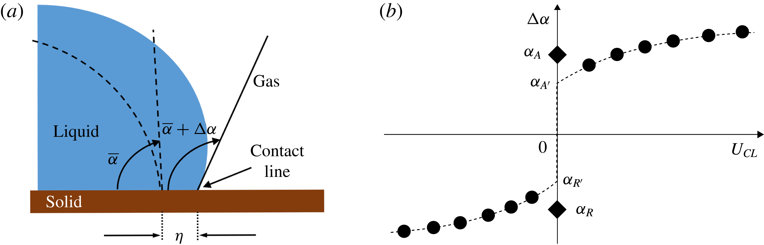
(a) Reference drop configuration (dashed), having reference contact angle
 $\overline{\unicode[STIX]{x1D6FC}}$
(see § 6), is disturbed to new shape (filled) with new angle
 $\unicode[STIX]{x1D6FC}\equiv \overline{\unicode[STIX]{x1D6FC}}+\unicode[STIX]{x0394}\unicode[STIX]{x1D6FC}$
, while the contact line is displaced a distance
 $\unicode[STIX]{x1D702}$
. (b) CL behaviour reported in the traditional diagram (TD),
 $\unicode[STIX]{x0394}\unicode[STIX]{x1D6FC}$
versus
 $U_{CL}\equiv \text{d}\unicode[STIX]{x1D702}/\text{d}t$
, after Dussan (Reference Dussan1979). Shorthand for
 $\unicode[STIX]{x0394}\unicode[STIX]{x1D6FC}_{A}$
is
 $\unicode[STIX]{x1D6FC}_{A}$
, and so forth.

When disturbed from a reference configuration, the CL and contact angle (CA) will deviate by a displacement
 $\unicode[STIX]{x1D702}$
and an angle
 $\unicode[STIX]{x0394}\unicode[STIX]{x1D6FC}$
, respectively, figure 1(a). Moving CL behaviour has been traditionally reported as
 $\unicode[STIX]{x0394}\unicode[STIX]{x1D6FC}$
versus
 $U_{CL}$
, figure 1(b), which we refer to as the traditional diagram (TD). According to figure 1(b), starting from the reference configuration,
 $\unicode[STIX]{x0394}\unicode[STIX]{x1D6FC}=0$
, the CL begins to advance (A) or recede (R) at angles
 $\unicode[STIX]{x1D6FC}_{A}$
(
 $\unicode[STIX]{x0394}\unicode[STIX]{x1D6FC}_{A}$
) and
 $\unicode[STIX]{x1D6FC}_{R}$
(
 $\unicode[STIX]{x0394}\unicode[STIX]{x1D6FC}_{R}$
). Slightly different values are obtained by slowing to the reference configuration, denoted
 $\unicode[STIX]{x1D6FC}_{A^{\prime }}$
and
 $\unicode[STIX]{x1D6FC}_{R^{\prime }}$
, respectively, indicating hysteresis. Our study cyclically forces a drop and uses high-speed imaging to obtain time series of
 $U_{CL}$
,
 $\unicode[STIX]{x0394}\unicode[STIX]{x1D6FC}$
and
 $\unicode[STIX]{x1D702}$
. Plotting
 $\unicode[STIX]{x0394}\unicode[STIX]{x1D6FC}$
against
 $U_{CL}$
results in a figure like figure 1(b). This serves as a familiar starting point for the reader. We then plot the same triplet of data in a number of different diagrams which reveals surprising features of the cyclic measurements.
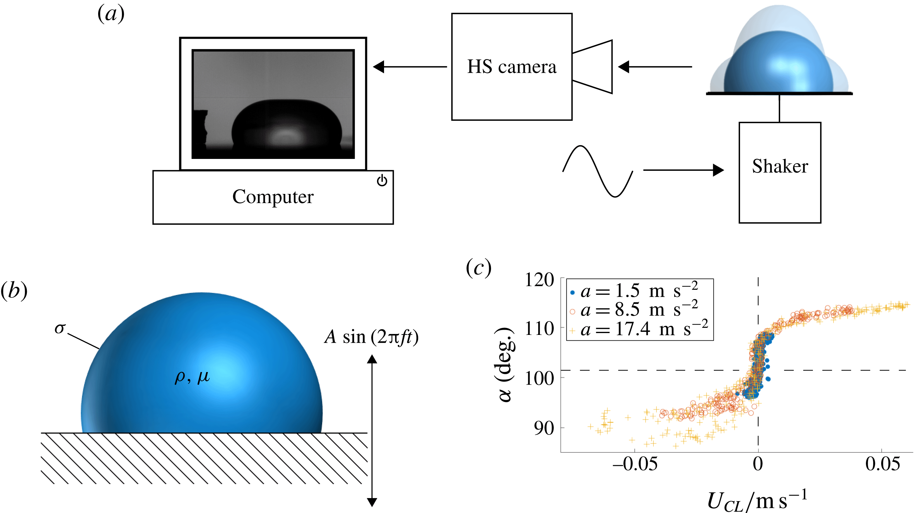
Our experimental set-up includes a droplet shaker and high-speed camera to image the contact-line region for subsequent analysis by computer, figure 2(a). The support plate is mechanically oscillated at frequency
 $f$
with laboratory frame plate-normal displacement
 $X(t)=A\sin (2\unicode[STIX]{x03C0}ft)$
to yield peak plate accelerations
 $a=\pm A(2\unicode[STIX]{x03C0}f)^{2}$
, where
 $A$
is the forcing amplitude and
 $t$
the time, figure 2(b). The CL response of water so-generated is shown in the traditional diagram, figure 2(c). Note that the classical sigmoidal shape of figure 1(b) is reproduced. For a 10-fold range of accelerations, the data reasonably collapse. Greater spread of data for the receding as compared to the advancing CL regime is consistent with prior observations (Elliott & Riddiford Reference Elliott and Riddiford1967). Our interest is in the regions away from the stationary CL, where CA multiplicity occurs, since these are the regions of high CL speeds.
(a) Set-up: signal drives shaker as HS camera images dynamic shapes for analysis. (b) Platform support oscillates with amplitude
 $A$
to drive drop of density
 $\unicode[STIX]{x1D70C}$
, dynamic viscosity
 $\unicode[STIX]{x1D707}$
and surface tension
 $\unicode[STIX]{x1D70E}$
,
 $X(t)=A\sin (2\unicode[STIX]{x03C0}ft)$
. (c) CL response in TD, for three accelerations
 $a$
, system M00.

Large CL excursions are favoured by low viscosity liquids on low-hysteresis coatings. Such liquids tend to have neutral affinity for the support; that is, a CA near
 $90^{\circ }$
. Our benchmark system for this study is water on a silicon wafer treated with a silane coating to achieve a rest-state CA,
 $\overline{\unicode[STIX]{x1D6FC}}\approx 101^{\circ }$
, with low CA hysteresis,
 $\unicode[STIX]{x1D6FC}_{A}-\unicode[STIX]{x1D6FC}_{R}\approx 2^{\circ }$
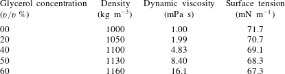
(Krumpfer & McCarthy Reference Krumpfer and McCarthy2010). We refer to this as the M00 system, according to water (‘00’ % glycerol) which is mobilized (M) by the silane coating. System M00 behaviour is exhibited in figure 2(c). The relatively narrow hysteresis loop suggests little dissipation, at least according to the traditional diagram. We also study more viscous water–glycerol mixtures (20 %, 40 %, 50 % and 60 % glycerol) and less mobile coatings (F, fluorinated) to compare against this benchmark. For a detailed description of systems used in this study and their preparation, see tables 3 and 4, § 3.
Relevant dimensional scales are given in table 1. To stay below the capillary length scale, small droplets are used. The volume-based length
 $D\equiv V^{1/3}$
, where
 $V$
is the drop volume, is approximately 2.7 mm for a drop volume of
 $V=20~\unicode[STIX]{x03BC}\text{}$
. This drop resonates at a measured frequency of approximately
 $f=67~\text{Hz}$
, yielding a time scale
 $1/\unicode[STIX]{x1D714}$
of approximately 2.4 ms, table 1. In comparison, the typical capillary time scale
 $\unicode[STIX]{x1D70F}\equiv \sqrt{\unicode[STIX]{x1D70C}V/\unicode[STIX]{x1D70E}}$
is approximately 7 times longer. Alternative length scales include the typical plate excursion,
 $A^{\ast }$
, and the viscous layer thickness
 $\unicode[STIX]{x1D6FF}\equiv \sqrt{\unicode[STIX]{x1D708}/\unicode[STIX]{x1D714}}$
which is approximately 0.05 mm. Note that this characteristic viscous layer is approximately half
 $A^{\ast }$
and approximately
 $1/50$
the scale
 $D$
. The comparison with
 $D$
suggests that the viscous layer plays a limited role in the dynamics, at least for water. The observed CL velocity scale
 $U_{CL}$
is approximately 50 % greater than the forcing velocity
 $A^{\ast }\unicode[STIX]{x1D714}$
, attributed to the effectiveness of resonant excitation and to the low-hysteresis nature of the support coating. Finally, the typical acceleration is also approximately 50 % greater than the acceleration of gravity. This suggests that significant deformation from the spherical cap shape may be expected.
Dimensionless characterizations can be based on either the forced motion (subscript ‘
 $f$
’) or the observed CL motion (subscript ‘
 $o$
’), table 2. Observed scales (e.g.
 $U_{CL}$
) often tend to better reflect the fluid dynamics but table 1 for our experiments suggests little difference. Inertial–capillary spreading is characterized by
 $Re\gg 1$
and
 $Ca_{o}\ll 1$
, as holds for M00. For both
 $We_{o}$
and
 $Ca_{o}$
characterizations, the local driving force for CL motion is the CA deviation,
 $\unicode[STIX]{x0394}\unicode[STIX]{x1D6FC}$
, which is more accurately characterized as
 $\unicode[STIX]{x1D70E}\sin (\unicode[STIX]{x0394}\unicode[STIX]{x1D6FC}_{max})$
rather than simply
 $\unicode[STIX]{x1D70E}$
. For
 $\unicode[STIX]{x0394}\unicode[STIX]{x1D6FC}_{max}\sim 10^{\circ }$
, table 1, the typical values listed in table 2 are increased by nearly a factor of six. The
 $Ca_{o}$
remains small but the revised
 $We_{o}$
for M00 is much closer to one, consistent with the balance of inertia and capillarity in these motions.
Scales: forcing,
 $\unicode[STIX]{x1D714}^{-1}\equiv (2\unicode[STIX]{x03C0}f)^{-1}$
; capillary,
 $\unicode[STIX]{x1D70F}\equiv \sqrt{\unicode[STIX]{x1D70C}V/\unicode[STIX]{x1D70E}}$
; volume-based length,
 $D\equiv V^{1/3}$
; typical forcing amplitude,
 $A^{\ast }$
; boundary layer thickness,
 $\unicode[STIX]{x1D6FF}\equiv \sqrt{\unicode[STIX]{x1D708}/\unicode[STIX]{x1D714}}$
; forcing speed,
 $A^{\ast }\unicode[STIX]{x1D714}$
, CL speed,
 $U_{CL}$
; forcing acceleration
 $A^{\ast }\unicode[STIX]{x1D714}^{2}$
; maximum angle-deviation,
 $\unicode[STIX]{x0394}\unicode[STIX]{x1D6FC}^{\ast }$
; asterisk (
 $^{\ast }$
) denotes value fixed throughout the paper, a typical value used for scaling.

Parameters, systems M00, F00: dimensional, drop of volume
 $V$
driven at frequency
 $f$
and acceleration
 $a$
; dimensionless: definitions below symbols (subscripts:
 $f=$
‘forcing’,
 $o=$
‘observed’), volume–length
 $D\equiv V^{1/3}$
; note that
 $U_{CL}$
is a maximum; for system definitions, cf. table 4.

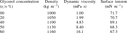
Water–glycerol mixture properties. Density and viscosity values based on empirical correlation (Cheng Reference Cheng2008). Surface tension values based on interpolation of experimental data (Glycerine Producers’ Association 1963).



1.1 Literature
There are many reviews of CL behaviour that include some combination of modelling, computation and measurement (Diez, Kondic & Bertozzi Reference Diez, Kondic and Bertozzi2000; Pomeau Reference Pomeau2001; Bonn et al. Reference Bonn, Eggers, Indekeu and Meunier2009; Savva & Kalliadasis Reference Savva and Kalliadasis2011; Snoeijer & Andreotti Reference Snoeijer and Andreotti2013). Scarce mention of inertial–capillary CL motions is found in these. Snoeijer & Andreotti (Reference Snoeijer and Andreotti2013) summarizes the situation where inertial–capillary behaviour is listed under future issues – ‘new challenges for moving contact lines emerge from the …inclusion of liquid inertia’.
Our literature review focuses on experimental work, justified by our paper’s focus on experiment. Inertial–capillary motion may be generated ‘naturally’ as in spreading by gravity (or capillarity) or be ‘forced’ as by a moving boundary. A traditional example of natural spreading occurs when gravity moves a drop down an inclined substrate (Mahadevan & Pomeau Reference Mahadevan and Pomeau1999; Aussillous & Quéré Reference Aussillous and Quéré2004; Hodges, Jensen & Rallison Reference Hodges, Jensen and Rallison2004). However, inertial motions may be the exception in such a set-up. Rapid natural transient motion driven by capillarity occurs in spreading on contact with a substrate (Bird, Mandre & Stone Reference Bird, Mandre and Stone2008; Carlson, Bellani & Amberg Reference Carlson, Bellani and Amberg2012; Winkels et al. Reference Winkels, Weijs, Eddi and Snoeijer2012). Interest in these measurements has often been in the power law exponents characterizing the various spreading regimes. Sometimes, the relaxation of a contact line from an initial non-equilibrium configuration is aided by vibrational energy input (Andrieu, Sykes & Brochard Reference Andrieu, Sykes and Brochard1994; Decker & Garoff Reference Decker and Garoff1996). Other kinds of forces used to drive transient inertial spreading include evaporation (e.g. Moffat, Sefiane & Shanahan Reference Moffat, Sefiane and Shanahan2009), impact (e.g. Yokoi et al. Reference Yokoi, Vadillo, Hinch and Hutchings2009), electromagnetic (e.g. Kocourek et al. Reference Kocourek, Karcher, Conrath and Schulze2006) and electrostatic (e.g. Sen & Kim Reference Sen and Kim2009) forces.
Steady CL motions result from steady forcing motions. To achieve these, a set-up that plunges a tape into a liquid bath has been favoured by the coating flows community (Blake & Ruschak Reference Blake and Ruschak1979). An advantage of this approach is that displacement (speed) rather than force (acceleration) is controlled and hence behaviour far from stick-slip can be readily achieved (Shen & Ruth Reference Shen and Ruth1998; Blake Reference Blake2006; Kumar & Prabhu Reference Kumar and Prabhu2007). In their experiments, Perlin and co-authors (Ting & Perlin Reference Ting and Perlin1995; Jiang, Perlin & Schultz Reference Jiang, Perlin and Schultz2004; Perlin, Schultz & Liu Reference Perlin, Schultz and Liu2004) drive a plunging plate in a cyclic manner. These studies report contact angle versus contact-line velocity diagrams that are more complicated than figure 1(b), probably owing to the additional influence of gravity. Prior experimental studies that drive sessile drops cyclically using vertical vibration have devoted some attention to moving CLs (e.g. Noblin, Buguin & Brochard-Wyart Reference Noblin, Buguin and Brochard-Wyart2004; Oh, Ko & Kang Reference Oh, Ko and Kang2008; Noblin, Buguin & Brochard-Wyart Reference Noblin, Buguin and Brochard-Wyart2009). For larger and flatter drops than ours, the focus has been on stick-slip CL behaviour, modelled as a dry friction oscillator (Noblin et al. Reference Noblin, Buguin and Brochard-Wyart2004). A subsequent paper extends to driving amplitudes and frequencies where non-axisymmetric modes are excited (Noblin et al. Reference Noblin, Buguin and Brochard-Wyart2009). The interesting idea of using vibration to induce CL motions in order to experimentally measure equilibrium contact angles has also been proposed in this paper.
Regarding the terminology ‘mobility’, some clarification is in order. Prior modelling and computational studies have introduced a function
 $g(x)$
, viewed as a single-valued representation of the CL behaviour,
 $\unicode[STIX]{x0394}\unicode[STIX]{x1D6FC}=g(U_{CL})$
with
 $0=g(0)$
(cf. figure 1
b). The Tanner (Reference Tanner1979) or Kistler–Hoffmann correlations (Schweizer & Kistler Reference Schweizer and Kistler2012) might be so-modelled. Linearization about the rest-state contact angle,
 $\unicode[STIX]{x0394}\unicode[STIX]{x1D6FC}=0$
, yields,
 $$\begin{eqnarray}\unicode[STIX]{x0394}\unicode[STIX]{x1D6FC}=\unicode[STIX]{x1D6EC}U_{CL}\quad \text{or}\quad M\unicode[STIX]{x0394}\unicode[STIX]{x1D6FC}=U_{CL}\quad \text{where }M\equiv \unicode[STIX]{x1D6EC}^{-1},\end{eqnarray}$$
with
 $\unicode[STIX]{x1D6EC}\equiv g^{\prime }(0)$
. Davis (Reference Davis1980) seems to have first introduced a
 $\unicode[STIX]{x1D6EC}$
-like parameter, in his modelling of the moving CL of a meandering rivulet. Beginning with Hocking’s use of this condition, it became known as the ‘Hocking condition’ even though Hocking attributed it to Davis (Hocking Reference Hocking1987). Borkar & Tsamopoulos (Reference Borkar and Tsamopoulos1991) refer to it as a ‘phenomenological parameter’, a ‘property’ of the materials involved, in their numerical study of liquid bridge oscillations. Lyubimov, Lyubimova & Shklyaev (Reference Lyubimov, Lyubimova and Shklyaev2004, Reference Lyubimov, Lyubimova and Shklyaev2006) call
 $\unicode[STIX]{x1D6EC}$
the ‘wetting parameter’ while Fayzrakhmanova & Straube (Reference Fayzrakhmanova and Straube2009) use both terms, ‘Hocking condition’ and ‘wetting parameter’, in computational studies of vibrated inviscid drops. All these studies treat
 $\unicode[STIX]{x1D6EC}$
as a way to model CL behaviour without complications of the observed multiplicity of contact angles for a given CL speed (hysteresis and associated nonlinearity).
We use the term ‘mobility’ in analogy with a particle subject to a force
 $F$
that moves with a velocity
 $U$
,
 $MF=U$
. In Stokes flow
 $M$
is called the ‘Stokes mobility’ and is just the inverse of the drag coefficient,
 $M=U/F=1/(6\unicode[STIX]{x03C0}\unicode[STIX]{x1D707}R)$
. In the CL case, the uncompensated Young–Dupré force acts around the perimeter (radius
 $R$
) in a direction tangent to the substrate,
 $$\begin{eqnarray}F=2\unicode[STIX]{x03C0}R\unicode[STIX]{x1D70E}[\cos \overline{\unicode[STIX]{x1D6FC}}-\cos (\overline{\unicode[STIX]{x1D6FC}}+\unicode[STIX]{x0394}\unicode[STIX]{x1D6FC})].\end{eqnarray}$$
If this is thought of as driving the CL motion, then
 $U_{CL}$
is given by,
 $F=\unicode[STIX]{x1D706}U_{CL}$
, where
 $\unicode[STIX]{x1D706}$
is the resistance or CL drag coefficient. In the case of small disturbances
 $\unicode[STIX]{x0394}\unicode[STIX]{x1D6FC}$
and near-neutral wetting,
 $\overline{\unicode[STIX]{x1D6FC}}\approx \unicode[STIX]{x03C0}/2$
, equation (1.2) reduces to
 $F\approx 2\unicode[STIX]{x03C0}R\unicode[STIX]{x1D70E}\unicode[STIX]{x0394}\unicode[STIX]{x1D6FC}$
and
 $M\equiv 2\unicode[STIX]{x03C0}R\unicode[STIX]{x1D70E}/\unicode[STIX]{x1D706}$
. In summary, our mobility
 $M$
formally satisfies (1.1) but our measurements that yield
 $M$
are away from the stick-slip region so a different interpretation is appropriate. Mobility is the ease with which a liquid rapidly wets or unwets a solid support. It is the inverse of the CL drag coefficient. This perspective notwithstanding, in this paper we purposely avoid any reliance on theory in order to emphasize that our measurement procedure stands alone, independent of assumptions.
We begin by outlining the experimental procedure in § 2 and detailing the materials and methods in § 3. Section 4 follows with the basic experimental measurements presented in several different ways to highlight the distinctions between the regimes of motion. We propose in § 5 the cyclic diagram which allows measurement of CL mobility, as detailed in § 6. Section 7 discusses the robustness and generality of the proposed measurement procedure by looking at additional results. Finally, some concluding remarks are given in § 8.
2 Experimental overview
In this work, rapid contact-line motions are induced by forcing the drop near resonance. Prior studies (e.g. Whitehill, Neild & Stokes Reference Whitehill, Neild and Stokes2012) have driven drops in a similar fashion in order to observe spreading transients but do not study cyclic CL behaviour while other studies (e.g. Vukasinovic, Smith & Glezer Reference Vukasinovic, Smith and Glezer2007) have driven drops near resonance in order to achieve atomization but do not study CL behaviour.
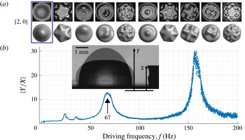
(a) Selected mode shapes resulting from excitation: photos (top) from experiment and rendered (bottom) from theory; the mode
 $[2,0]$
(boxed) is excited in this study; drop footprint radius
 ${\approx}2.5~\text{mm}$
(Bostwick & Steen Reference Bostwick and Steen2014; Chang et al.
Reference Chang, Bostwick, Daniel and Steen2015). (b) Response of a
 $20~\unicode[STIX]{x03BC}\text{l}$
drop to frequency scan excitation where
 $|Y/X|$
is normalized drop apex response. Inset: shape extremes (superimposed), platform displacement
 $X$
and drop apex displacement
 $Y$
.
 $X$
and
 $Y$
are measured in laboratory frame. System M00.

Shapes of various modes that resonate at different frequencies are shown in figure 3(a). In this study, we excite the
 $[2,0]$
mode exclusively as it yields the most efficient coupling to CL motions. The resonant frequency for
 $[2,0]$
mode is observed experimentally from the maximum in drop apex deflection,
 $Y$
, by a frequency sweep. Figure 3(b) provides an example. At this volume, the resonant peak of mode
 $[2,0]$
occurs at
 ${\sim}67~\text{Hz}$
while the higher peak is at
 ${\sim}155~\text{Hz}$
and corresponds to mode
 $[4,0]$
. The two small peaks at
 ${\sim}23$
and
 ${\sim}35~\text{Hz}$
are subharmonic responses, placed outside the scope of this work. Our frequency sweep response is qualitatively similar to that obtained computationally by Korenchenko & Malkova (Reference Korenchenko and Malkova2015) with the notable difference that our
 $[2,0]$
peak is weaker than the
 $[4,0]$
peak. Based on the findings of Lyubimov et al. (Reference Lyubimov, Lyubimova and Shklyaev2006) and our observations that the
 $[2,0]$
mode exhibits considerable CL motion while
 $[4,0]$
exhibits none, we believe this difference is the result of contact-line dissipation, precluded by the boundary conditions used in Korenchenko & Malkova (Reference Korenchenko and Malkova2015). To excite CL motions,
 $f$
(or
 $\unicode[STIX]{x1D714}\equiv 2\unicode[STIX]{x03C0}f$
) is fixed near the
 $[2,0]$
resonance. Driving parameters are summarized in table 2. For error analysis, see section SM1 (supplementary material available online at https://doi.org/10.1017/jfm.2018.105).
3 Materials and methods
3.1 Materials
Trimethylsiloxy terminated poly(dimethylsiloxane) (PDMS) (Gelest, Product Code DMS-T22-100GM) was purchased from Gelest (Morrisville, PA). Silicon wafers (Silicon Quest International, catalogue no. 808-007) were purchased from Silicon Quest International (San Jose, CA). Sulphuric acid (95–98 % min., MW 98.08, CAS#7664-93-9), toluene (99.5 % min., MW 92.14, CAS#108-88-3) and acetone (CAS#67-64-1; Macron Chemicals) were purchased from VWM International (Radnor, PA). Hydrogen peroxide solution (50 wt.%, SKU 516813-500ML, CAS#7722-84-1, MW
 $34.01~\text{g}~\text{mol}^{-1}$
) was purchased from Sigma-Aldrich (St. Louis, MO). High-purity compressed nitrogen was purchased from Airgas (Radnor, PA). Glass vials (20 ml borosilicate glass scintillation vial, catalogue no. 03-337-5) and light mineral oil (CAS#8042-47-5) were purchased from Fisher Scientific (Pittsburgh, PA).
Relevant properties of the liquids used in this work are given in table 3. Designations and key characterizations of solid–liquid systems are given in table 4.
3.2 Preparation of surfaces
To prepare substrate
 $M$
, a silicon chip with dimensions of approximately
 $2\times 1~\text{cm}$
is cleft from a silicon wafer and sonicated (Ultrasonic Cleaner, model B2500A-DTH, VWR) in water for 20 min to remove solid particles on the surface. Any organic contaminants are then removed by soaking the chip in piranha solution (70 % sulphuric acid/30 % hydrogen peroxide) for 20 min. The chip is rinsed in running de-ionized (DI) water (purified by an Elga Ultra SC MK2, Siemens) for 10 min, blow dried using high-purity compressed nitrogen and cleaned using oxygen plasma (Basic Plasma Cleaner, model PDC-32G, Harrick Plasma) at
 $600~\unicode[STIX]{x03BC}\text{m}$
for 1 min. The chip is placed in a freshly opened glass vial and wet with as-received PDMS. The vial is capped and baked at
 $100\,^{\circ }\text{C}$
for 24 h. After the vial cools to room temperature, the substrate is rinsed in turn with toluene, acetone and DI water.
3.3 Characterization of surfaces
Contact angle measurements are performed using an in-house MATLAB code and spot checked with a commercial goniometry software, DROPimage Advanced (Ramé-Hart Instrument Co., Succasunna, NJ). An error analysis (SM1) puts the uncertainty in the CA measurement code at
 $\pm 1^{\circ }$
.
3.4 Mechanical and imaging equipment
A system consisting of a function generator (Agilent 33220A, Agilent Technologies, Santa Clara, CA), a power amplifier (Crown CE2000, Crown Audio, Elkhart, IN) and a mechanical vibrator (PASCO SF-9324, PASCO, Roseville, CA) similar to that used by Chang et al. (Reference Chang, Bostwick, Steen and Daniel2013) is responsible for generating the mechanical vibrations. The solid sample surfaces are mounted horizontally on the vibrator. A manual microsyringe (Gilmont GS 1200, Cole-Parmer, Vernon Hills, IL) is used to dispense the test liquids. Typically, drops of
 $20~\unicode[STIX]{x03BC}\text{l}$
are used.
A RedLake HG-XL imaging system (DEL Imaging Systems, Cheshire, CT) fitted with a Tamron SP AF 90mm f/2.8 Di Macro Lens (Tamron USA, Inc., Commack, NY) is used to capture high-speed, side view images of the experiment. Typical frame rates used are in the range of 2000–5000 Hz. The typical spatial resolution is
 $10~\unicode[STIX]{x03BC}\text{m}~\text{pixel}^{-1}$
.
3.5 Image analysis
The useful measurements of the experiment are derived from the side view profile of the drop, supplemented by the measurement of support displacement. For instance, the contact-line velocity is approximated by the numerical time derivative of the drop profile where it joins the substrate. Meanwhile, the contact angle is measured using the tangent line of the drop profile at the contact line, as approximated using a secant method.
3.6 Data reduction
Where quantities are said to be scaled, the scaling factors are as follows (cf. table 1). Length scale:
 $A^{\ast }=0.1~\text{mm}$
; time scale:
 $\unicode[STIX]{x1D70F}^{\ast }=17~\text{ms}$
; angular scale:
 $\unicode[STIX]{x0394}\unicode[STIX]{x1D6FC}^{\ast }=10^{\circ }$
.
Where plots are given in red, blue and green colours, the colour coding denotes the following. Blue:
 $|U_{CL}|/\max (U_{CL})>0.6$
, green:
 $0.1<|U_{CL}|/\max (U_{CL})<0.6$
, red:
 $|U_{CL}|/\max (U_{CL})<0.1$
. The lower threshold value of 0.1 is arbitrarily chosen while the determination of the upper threshold of 0.6 will be discussed in § 5. The degree of ambiguity and arbitrariness in the evaluation of our final result of interest, the mobility parameter, is detailed in SM1.3, with the relative uncertainty typically within
 $\pm 3\,\%$
.
4 Contact-line response: stick, shoulder and wing regions
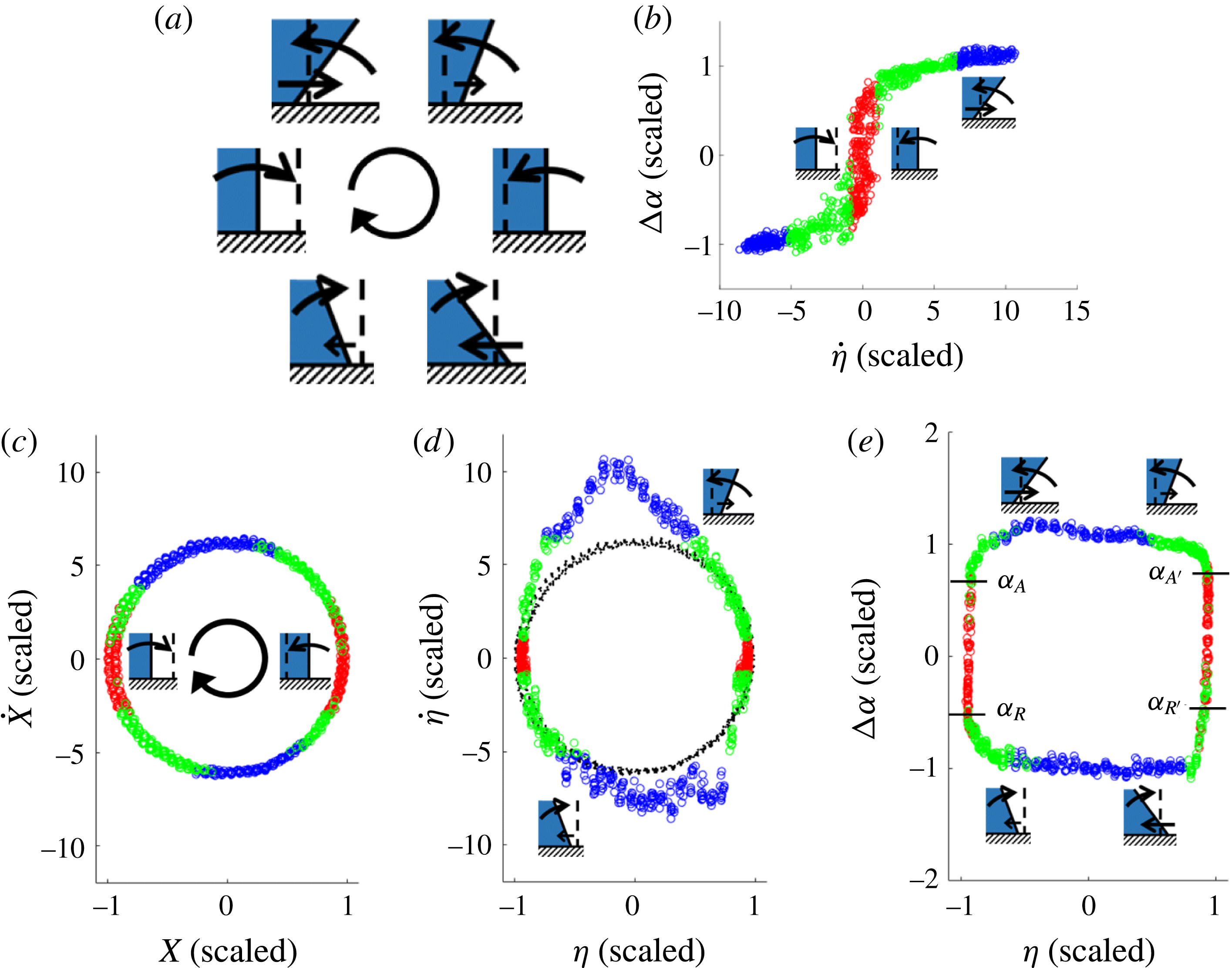
(a) Sketches of CL position, CA tangent and directions-of-change (doc): vertical dashed line indicates CL rest position and CA rest tangent; straight arrows represent doc of CL, curved arrows, doc of CA; clockwise time (centre arrow). (b) Traditional diagram (TD), data coloured by stick, shoulder and wing region. (c) Platform phase plane: clockwise time. (d) CL phase plane:
 $\dot{\unicode[STIX]{x1D702}}$
versus
 $\unicode[STIX]{x1D702}$
(coloured),
 ${\dot{X}}$
versus
 $X$
(black) from (c), for reference. (e) CA versus CL diagram. All plots have the same scales: length
 $A^{\ast }\equiv 0.1~\text{mm}$
; time
 $\unicode[STIX]{x1D70F}^{\ast }=0.17~\text{s}$
; angles
 $\unicode[STIX]{x0394}\unicode[STIX]{x1D6FC}^{\ast }\equiv 10^{\circ }$
. 12 cycles. M00 system.

The motion of the contact line in response to cyclic excitation is shown in six snapshot schematics in figure 4(a). The vertical dashed line, fixed in the platform frame, is a reference for the CL rest position and the CA rest tangent. The CA rest tangent is vertical since the rest CA is taken to be
 $\overline{\unicode[STIX]{x1D6FC}}=90^{\circ }$
, for simplicity. The displacement
 $\unicode[STIX]{x1D702}$
, contact angle
 $\unicode[STIX]{x1D6FC}$
and their directions-of-change (straight arrow,
 $\unicode[STIX]{x1D702}$
; curved arrow,
 $\unicode[STIX]{x1D6FC}$
) are shown for one cycle of the platform motion. Extremes of displacement occur at the 3 and 9 o’clock positions. These correspond to sticking where the CL pins while the CA changes. Extremes of
 $\unicode[STIX]{x0394}\unicode[STIX]{x1D6FC}$
occur near the 11 and 5 o’clock positions, at instants when the angle changes direction. Selected schematics are added judiciously to subsequent plots to guide the reader. Figure 4(b) reproduces a subset of the data in figure 2(c). The stick region has been coloured red, the shoulders green and the wings blue. In this way, the colour of each data point in figure 4(b) defines its identity. Different mappings of the data of figure 4(b), retaining their colours, are reported in figure 4(c–e). That is, figure 4(c–e) consists of three re-plots of the data of the traditional diagram (TD), figure 4(b). Figure 4(c,d) are platform and CL displacement phase-plane plots, while figure 4(e) is mixed CA–CL displacement diagram.
Figure 4(c) plots the platform phase plane,
 ${\dot{X}}$
versus
 $X$
. (Note that the axes have different scales to make the plot circular. This different scaling of axes counters our scaling of time in
 ${\dot{X}}$
(
 $y$
-axis) by the capillary time
 $\unicode[STIX]{x1D70F}^{\ast }$
rather than by the resonance time
 $(2\unicode[STIX]{x03C0}f)^{-1}$
. That is, if the resonance time were properly used instead, the plot would naturally be circular.) The circular shape shows that simple harmonic motion has been mechanically achieved by the shaker table, to a good approximation. The stick regions correspond to extremes of displacement (
 ${\dot{X}}=0$
) and the wing regions to extremes of speed (
 $X=0$
). This mapping serves as the clock for the cyclic CL motion. Sticking (red) is estimated to occupy 26 %, the shoulders (green) 38 % and the wings (blue) 36 % of a driving period. Moreover, these regions are nearly in phase with the driving motion, suggesting that damping plays little role in the response.
Figure 4(d) shows the phase plane of
 $\unicode[STIX]{x1D702}$
versus
 $\dot{\unicode[STIX]{x1D702}}$
with the clock as reference (same scales). The black circle is deformed to the coloured loop. The deviation from a circle in the CL phase plane is a measure of the deviation of the CL motion from harmonic oscillation. The asymmetry about the horizontal axis speaks to the difference between advancing/receding CL. The asymmetry about the vertical axis speaks to the phase lead/lag of the advancing/receding CL. Overall, the mapping of the circle to the deformed loop reveals a characterization of the CL response. Notable features are that (i) while both advancing and receding, the greatest
 $\dot{\unicode[STIX]{x1D702}}$
occurs nearby but does not coincide with
 $\unicode[STIX]{x1D702}=0$
; and that (ii) the distortion of the advancing wing is greater (and sharper) than that of the receding wing.
Figure 4(e) plots the remaining combination of the three observables
 $\unicode[STIX]{x0394}\unicode[STIX]{x1D6FC}$
versus
 $\unicode[STIX]{x1D702}$
. This highlights the cyclic
 $\unicode[STIX]{x0394}\unicode[STIX]{x1D6FC}$
behaviour. Most strikingly, the loop has become nearly rectangular with slightly rounded shoulders. Thus, we see that CA behaviour is dominated by stick (red) and wing (blue) regions. However, a perfectly rectangular response would correspond to a constant
 $\unicode[STIX]{x0394}\unicode[STIX]{x1D6FC}$
along each wing segment. A closer look suggests that
 $\unicode[STIX]{x0394}\unicode[STIX]{x1D6FC}$
decreases monotonically as the CL rapidly passes the reference position, both going and coming, which suggests that the loop is actually a sheared rectangle. In either case, the simplicity of how the stick and rapidly moving CL regions fit together is striking. The area within the loop is related to the CL dissipation per cycle (Xia, Daniel & Steen Reference Xia, Daniel and Steen2017). Finally, one also notes that advancing,
 $\unicode[STIX]{x1D6FC}_{A}$
and
 $\unicode[STIX]{x1D6FC}_{A}^{\prime }$
, and receding CAs,
 $\unicode[STIX]{x1D6FC}_{R}$
and
 $\unicode[STIX]{x1D6FC}_{R}^{\prime }$
, can easily be read off the diagram, as boundaries between red–green and green–red colour changes.
5 Unmasking the linearity of wing regions: the cyclic diagram
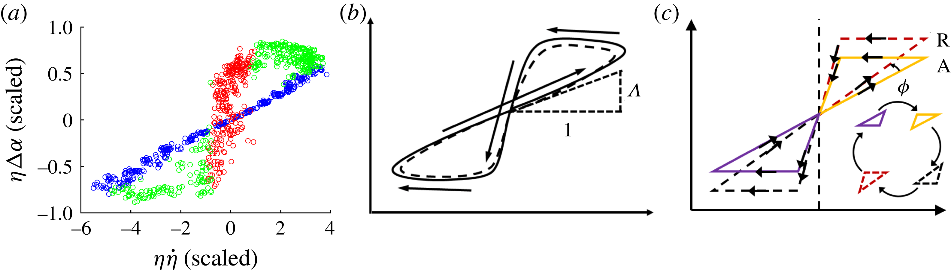
In figure 4(e), the two wing regions are observed to be two sides of an approximate quadrilateral. To study the wing behaviour more closely, we remap the data yet again. Within each of the two wing regions, figure 4(b), the reference position is traversed once. To map the wings into a neighbourhood of the origin, both axes of figure 4(b) are scaled by
 $1/\unicode[STIX]{x1D702}$
. The result is the diagram,
 $\unicode[STIX]{x1D702}\unicode[STIX]{x0394}\unicode[STIX]{x1D6FC}$
versus
 $\unicode[STIX]{x1D702}\dot{\unicode[STIX]{x1D702}}$
, figure 5(a). We call this the CL cyclic diagram, or simply cyclic diagram, a diagram that combines the three essential measurements,
 $\unicode[STIX]{x1D702}$
,
 $\dot{\unicode[STIX]{x1D702}}$
and
 $\unicode[STIX]{x0394}\unicode[STIX]{x1D6FC}$
. It is noted here that, in general, figure 5(a) requires a prerequisite ‘balancing’ step, which will be discussed below in § 6.
In the schematic version of the cyclic diagram, figure 5(b), the neighbourhood of the origin is crossed four times during a cycle while each of two loops (solid and dotted) is traversed just once. The presence of two loops per cycle is due to the advancing and receding phases of the driving period each tracing out a loop. In this case, the loops are of similar shape. The origin plays a double role, representing simultaneously (i) the reference- (
 $\unicode[STIX]{x1D702}=0$
) and (ii) the stick- (
 $\dot{\unicode[STIX]{x1D702}}=0$
) with mean angle (
 $\unicode[STIX]{x0394}\unicode[STIX]{x1D6FC}=0$
) positions. The super-harmonic feature of the cyclic diagram derives from the quadratic nature of the coordinates – if
 $\unicode[STIX]{x1D702}$
and
 $\dot{\unicode[STIX]{x1D702}}$
were approximated by a sine and cosine waves of the same frequency, respectively, then
 $\unicode[STIX]{x1D702}\dot{\unicode[STIX]{x1D702}}$
would be a sine wave of twice that frequency.
Remarkably, in the cyclic diagram the wing regions map to a single region passing through the origin, well approximated as linear. Note that the formation of this linear region is independent of any colouring scheme; it serves as the basis for identifying the wing region in the traditional diagram. The slope of this line represents a property of the traditional diagram since the same weighting factor,
 $\unicode[STIX]{x1D702}$
, is applied to both axes and thereby preserves the original information in the TD. This property, measured as the slope
 $\unicode[STIX]{x1D6EC}$
, is what we call the CL drag resistance or drag coefficient (inverse mobility), cf. figure 5(b). To appreciate its interpretation as a drag to CL motion, first consider the limit of
 $\unicode[STIX]{x1D6EC}\rightarrow \infty$
where figure 5(b) approaches a vertical line segment centred on the origin. This picture would imply that despite any change in CA, presumably brought about by applied forcing, there is no CL motion. The CL is pinned. In the opposite limit of
 $\unicode[STIX]{x1D6EC}\rightarrow 0$
, figure 5(b) approaches a horizontal line, so arbitrary CL motion can take place without any applied forcing. The CL is fully mobile.
Contact-line cyclic diagram. (a) A re-plot of data in figure 4(b) for the M00 system, axes weighted by
 $\unicode[STIX]{x1D702}$
(scales and colours as in figure 4). (b) Cyclic diagram schematic, the double-loop features one traverse (solid) followed by a second (dotted), time indicated by arrows. (c) CA balancing:
 $\overline{\unicode[STIX]{x1D6FC}}$
fit to minimize angle
 $\unicode[STIX]{x1D719}$
between advancing (A) and receding (R) loops; inset: visiting sequence of coloured triangles.

The interpretation of the two cyclic diagram loops is immediate. Start at the top of the red region in figure 5(a), say. For a CL that has just stopped receding,
 $\unicode[STIX]{x1D702}$
at this particular instant is at its negative extremum (
 $\unicode[STIX]{x1D702}<0$
). The CA then increases while the CL remains ‘in sticking mode’ (hysteresis), traversing vertically downwards through the red region. This corresponds to the sketch in the 9 o’clock position in figure 4(a). Eventually, the CL begins to advance as red turns to green, cf. 10 o’clock sketch in figure 4(a). The CL then accelerates and enters the linear region (blue) beginning at the bottom left corner. As the CL continues advancing through the reference position into positive territory (
 $\unicode[STIX]{x1D702}>0$
), cf. 12 o’clock sketch in figure 4(a), the advancement slows and blue turns to the green at the top right. Once advancement halts,
 $\unicode[STIX]{x1D702}$
is at its positive extremum (
 $\unicode[STIX]{x1D702}>0$
), cf. 3 o’clock sketch in figure 4(a), and the system returns to near our starting point. It is not actually our starting point however, since
 $\unicode[STIX]{x1D702}>0$
. The motions described so far only constitute the sticking–advancing phase cf. 9 through 3 o’clock sketches in figure 4(a). A sticking–receding phase follows, cf. 3 through 9 o’clock sketches in figure 4(a). Therefore, the full cycle of stick–advance–stick–recede would trace out yet another overlapping loop in the cyclic diagram. The two loops are illustrated schematically in figure 5(b), one solid and one dotted. Figure 5(c) will be discussed in the next section.
6 Mobility measurement and CA balancing
Mobility characterizes how CL speed
 $\dot{\unicode[STIX]{x1D702}}$
relates to CA deviation,
 $\unicode[STIX]{x0394}\unicode[STIX]{x1D6FC}\equiv \unicode[STIX]{x1D6FC}-\overline{\unicode[STIX]{x1D6FC}}$
, where
 $\overline{\unicode[STIX]{x1D6FC}}$
is a reference CA.
 $\overline{\unicode[STIX]{x1D6FC}}$
can be an evaluation of the equilibrium contact angle,
 $\overline{\unicode[STIX]{x1D6FC}}=\unicode[STIX]{x1D6FC}_{e}$
, say, or the average of advancing and receding angles,
 $\overline{\unicode[STIX]{x1D6FC}}=(\unicode[STIX]{x1D6FC}_{A}-\unicode[STIX]{x1D6FC}_{R})/2$
(cf. figure 1
b), taken from separate static measurements, or it can be left as a free parameter. We choose the latter to avoid attaching physical interpretation to the value without justification. For the low-hysteresis system M00, subsequent fitting yields
 $\overline{\unicode[STIX]{x1D6FC}}\approx \unicode[STIX]{x1D6FC}_{A}\approx \unicode[STIX]{x1D6FC}_{R}\approx \unicode[STIX]{x1D6FC}_{e}$
, so reference CA distinctions are lost in this case.
The slope of
 $\unicode[STIX]{x1D702}\unicode[STIX]{x0394}\unicode[STIX]{x1D6FC}$
versus
 $\unicode[STIX]{x1D702}U_{CL}$
characterizes the resistance to CL motion,
 $$\begin{eqnarray}\unicode[STIX]{x1D702}\unicode[STIX]{x0394}\unicode[STIX]{x1D6FC}=\unicode[STIX]{x1D6EC}\unicode[STIX]{x1D702}U_{CL}.\end{eqnarray}$$
In view of the mobility,
 $M\equiv 1/\unicode[STIX]{x1D6EC}$
, limits
 $M\rightarrow 0$
(
 $\unicode[STIX]{x1D6EC}\rightarrow \infty$
) describe a pinned CL and
 $M\rightarrow \infty$
(
 $\unicode[STIX]{x1D6EC}\rightarrow 0$
), a fully mobile CL, as mentioned in § 5. We shall report
 $\unicode[STIX]{x1D6EC}$
values below. In the absence of a molecular basis for scaling
 $\unicode[STIX]{x1D6EC}$
, we will scale empirically using length
 $D$
, time
 $\unicode[STIX]{x1D70F}^{\ast }$
and angle deviation
 $\unicode[STIX]{x0394}\unicode[STIX]{x1D6FC}^{\ast }$
, as provided in table 1.
Mobility
 $1/\unicode[STIX]{x1D6EC}$
is measured by doing a best fit of (6.1) to the wing data, using
 $\overline{\unicode[STIX]{x1D6FC}}$
as a free parameter. The best fit to the data of figure 5(a) yields
 $\overline{\unicode[STIX]{x1D6FC}}=101^{\circ }$
, identical to the static CA measured by conventional goniometer (table 4), within experimental error. For M00, one finds
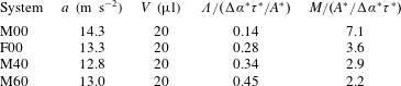
 $\unicode[STIX]{x1D6EC}=0.14\unicode[STIX]{x0394}\unicode[STIX]{x1D6FC}^{\ast }\unicode[STIX]{x1D70F}^{\ast }/A^{\ast }$
. This is the slope of the blue data through the origin of the cyclic diagram, figure 5(a). The value of
 $\unicode[STIX]{x1D6EC}=0.14\unicode[STIX]{x0394}\unicode[STIX]{x1D6FC}^{\ast }\unicode[STIX]{x1D70F}^{\ast }/A^{\ast }$
means that a
 $10^{\circ }$
change in CA corresponds to a
 $4.64~\text{cm}~\text{s}^{-1}$
change in CL speed. Over one driving cycle period of 16 ms, the total CA excursion amounts to about
 $\pm 10^{\circ }$
and the net excursion of the CL is approximately 0.2 mm.
One might expect that advancing and receding CLs wings, in general, could have different mobilities. This could well be the case if
 $\overline{\unicode[STIX]{x1D6FC}}$
is set to be an independently determined (or assumed) value. In place of figure 5(b), one would then find two loops of data, as shown in schematic in figure 5(c). The advancing (A) and receding (R) loops have different slopes passing through the origin. The angle
 $\unicode[STIX]{x1D719}$
between the linear segments is a measure of the deviation or asymmetry of advancing/receding behaviours. In the general case, with foreknowledge of the asymmetry
 $\unicode[STIX]{x1D719}$
, one could seek a 2-parameter fit for each of two resistances,
 $\unicode[STIX]{x1D6EC}_{A}$
and
 $\unicode[STIX]{x1D6EC}_{R}$
, but the foreknowledge requires information not readily available from existing measurement techniques.
In this paper, we eschew the need for any additional information or assumptions by contenting ourselves with an overall mobility characterization for both the advancing and receding regimes. The M00 system lends itself to this approach with its low hysteresis that makes it naturally symmetric (
 $\unicode[STIX]{x1D719}\sim 0$
). Our 1-parameter fit procedure is equivalent to minimizing angle
 $\unicode[STIX]{x1D719}$
in figure 5(c) over
 $\overline{\unicode[STIX]{x1D6FC}}$
. That is, we find the value of
 $\overline{\unicode[STIX]{x1D6FC}}$
that minimizes the R-squared value of a single-parameter fit (linear regression) over the linear region in figure 5(c). We refer to this procedure as ‘balancing the CA’, essentially a symmetrization procedure.
7 Results and discussion
Various response diagrams have been introduced in order to study the moving contact line during inertial–capillary wetting/unwetting motions. Each highlights different features.
The platform phase plane serves as a clock. It yields the fractions of the driving period that the motion spends in stick and wing regions. The mixing of colours indicates the relative regularity of the various regime transitions. There is some mixing at each transition yet the stick–slip and slip–stick transitions exhibit the most mixing, figure 4(c). The clock also confirms the extent to which the driving platform delivers a simple harmonic motion. By figure 4(c), our driving is harmonic to good approximation.
The CL phase plane reflects how the droplet filters the driving motion to the CL motion. Both amplitude and phase of the mapping from platform to CL motion carry information. Remarkably, amplitudes
 $\unicode[STIX]{x1D702}$
are of the same order as amplitudes
 $X$
while
 $U_{CL}$
is 2-fold greater than
 ${\dot{X}}$
, a benefit of resonance. The advancing wing (wetting) is more regular with greater amplitudes than the receding wing (unwetting), as noted by prior studies (e.g. Elliott & Riddiford Reference Elliott and Riddiford1967). Regarding phase difference, maximum speeds on advancing and receding wings both occur before platform maximums. New here is a means to measure the differences in regularity, with the benefit of multi-cyclic statistics. In summary, the mapping from the platform to the CL phase plane is a new and useful characterization of CL motions.
The mixed diagram, figure 4(e), yields yet another view of drop response. Here, the stick regions are naturally vertical yet, surprisingly, the wing regions are nearly horizontal and occupy most of the rest of the loop. That is, this mapping reveals the extent to which the stick and wing regions dominate the CA behaviour. The response might be productively modelled as a quadrilateral.
The CL cyclic diagram is distinguished by its quadratic nature. The axes in this diagram are scaled to bring the sweeping of the CL past the rest position into focus. The wing regions map to a linear segment whose inverse slope yields the mobility measurement. Definition of the wing regions, alternatively, could be specified in the cyclic diagram. The surprise then is that (i) the wing regions are linear to a good approximation and (ii) the linearity corresponds to a major fraction of the driving cycle.
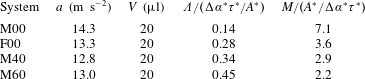
How is mobility influenced by the support affinity? An F00 system exhibits greater hysteresis,
 $\unicode[STIX]{x1D6FC}_{A}-\unicode[STIX]{x1D6FC}_{R}$
, and a higher static CA, table 4 and
 $\unicode[STIX]{x1D6EC}$
doubles from the M00 value, table 5. This greater resistance to mobility is consistent with the higher hysteresis due to surface chemistry. For the various F00 diagrams, see section SM2. These show an overall similarity to the M00 diagrams. Increasing bulk viscosity also decreases mobility, cf. M40 and M60, table 5. Note that identical volumes,
 $V$
, and similar accelerations,
 $a$
, are used.
The breadth of usefulness of the cyclic diagram (and dynamic balancing procedure) depends on the extent to which mobility is a material-like parameter, like viscosity given by a rheometer and used to make predictions in other flow geometries and contexts. This important consideration is beyond the scope of this paper. However, a necessary condition is that measured mobility parameters for driving drops near resonance be independent of details of our cyclic-dynamic protocol. Next, we argue this point.
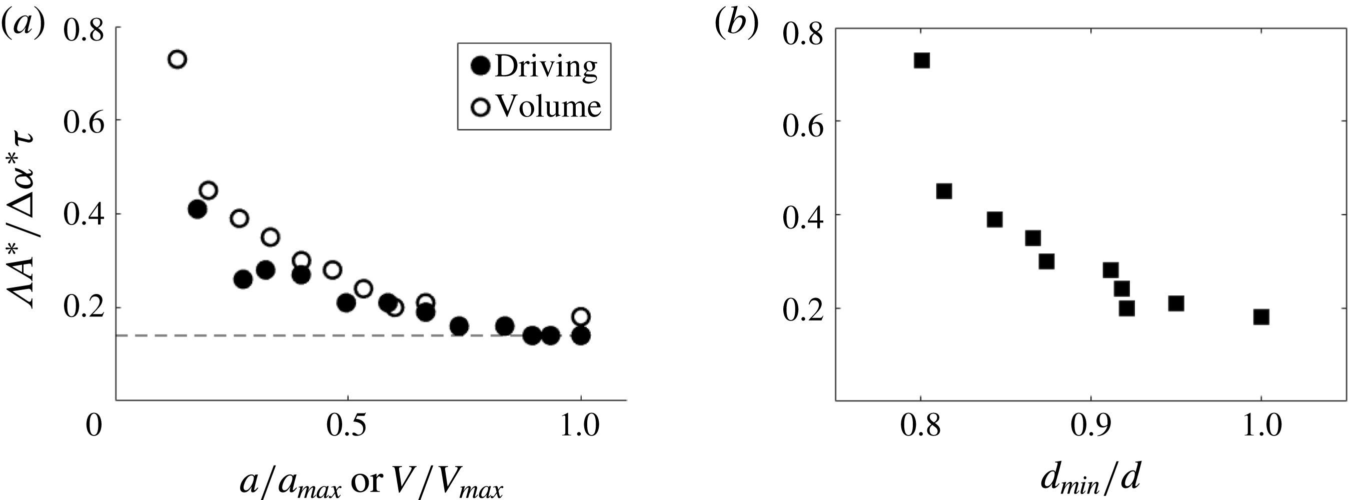
(a)
 $\unicode[STIX]{x1D6EC}$
versus acceleration
 $a$
, drop volume
 $V$
, all scaled. System M00. Scales:
 $a_{max}=15.3~\text{m}~\text{s}^{-2}$
for
 $20~\unicode[STIX]{x03BC}\text{l}$
drop;
 $V_{max}=30~\unicode[STIX]{x03BC}\text{l}$
. Horizontal line has
 $y$
-intercept at 0.14, cf. table 5; (b) scaled
 $\unicode[STIX]{x1D6EC}$
versus scaled boundary layer thickness
 $d\equiv \unicode[STIX]{x1D6FF}/D$
,
 $d_{min}=0.018$
, system M00, for
 $20~\unicode[STIX]{x03BC}\text{l}$
drop. Note that here,
 $\unicode[STIX]{x1D70F}$
, which appears in the
 $\unicode[STIX]{x1D6EC}$
scale, depends on
 $V$
, in contrast to table 5, where
 $\unicode[STIX]{x1D70F}^{\ast }$
is fixed.

Measured
 $\unicode[STIX]{x1D6EC}$
and
 $M$
for Mxx and F00 systems.
 $\unicode[STIX]{x0394}\unicode[STIX]{x1D6FC}^{\ast }\unicode[STIX]{x1D70F}^{\ast }/A^{\ast }=17~\text{s}\;^{\circ }~\text{cm}^{-1}$
.
To what extent is mobility independent of
 $V$
and
 $a$
? Capillary resonance depends on drop volume and large volumes invoke gravity. Additionally, higher accelerations distort shapes and influence CL behaviour. Minimal influence of gravity on capillarity is ensured by
 $Bo\equiv \unicode[STIX]{x1D70C}gD^{2}/\unicode[STIX]{x1D70E}\ll 1$
, and on driving acceleration by
 $g/a\ll 1$
, both limited by extreme shape distortions that come with higher accelerations that ultimately result in atomization.
For the M00 system, measured values of
 $\unicode[STIX]{x1D6EC}$
at varying driving acceleration and drop sizes are given in figure 6. For low enough driving acceleration or volume, the CL remains pinned, as expected given the stick–slip behaviour reported in prior literature (Noblin et al.
Reference Noblin, Buguin and Brochard-Wyart2004), and
 $\unicode[STIX]{x1D6EC}$
is not relevant (
 $\unicode[STIX]{x1D6EC}\rightarrow \infty$
). In figure 6(a), for moderate accelerations or volumes,
 $\unicode[STIX]{x1D70C}aD^{2}/\unicode[STIX]{x1D70E}\approx 1$
, and as driving acceleration or drop volume increases,
 $\unicode[STIX]{x1D6EC}$
approaches a plateau. In figure 6(b), we examine the viscous boundary layer thickness,
 $\unicode[STIX]{x1D6FF}=\sqrt{\unicode[STIX]{x1D708}/\unicode[STIX]{x1D714}}$
, similar to the Stokes boundary layer thickness (Batchelor Reference Batchelor1999), and scale by the drop size. The ratio
 $d\equiv \unicode[STIX]{x1D6FF}/D$
then gives a measure of the oscillatory boundary layer thickness relative to drop size. Figure 6(b) shows that, for small enough size, the relatively large thickness begins to influence scaled
 $\unicode[STIX]{x1D6EC}$
. The influences of small thickness, acceleration and volume are similar. The asymptotic behaviour of figure 6 is typical of the systems studied, suggesting a range where
 $\unicode[STIX]{x1D6EC}$
is independent of experimental protocol.
8 Concluding remarks
We experimentally study the motion of contact lines (CL) by driving a sessile water drop near resonance. The motions conform to classical CL behaviour, by the traditional diagram (TD). We then use the TD to identify stick and wing regions. The stick region starts (ends) at the onset of sticking (slipping) on a receding (advancing) CL. By colouring the data by region, one can observe how the TD maps to the CL cyclic diagram. For water on a neutrally wetting and low-hysteresis support, the cyclic diagram reveals a linear response of wing data which yields the CL mobility measurement.
Any system of partially wetting liquid and support can be tested by the procedure introduced here. Wing regions can be anticipated – they appear routinely in the nearly 50 years of reporting data in the TD format. Hence, our approach is of broadest applicability. What cannot be anticipated is a successful mobility measurement from the cyclic diagram.
Demonstrating how to measure mobility suggests a way around the long-standing difficulty, by way of reinterpretation, that systems that display CA hysteresis do not have a well-defined linearized stability theory (Davis Reference Davis1983). Mobility measurement has been demonstrated for water on support M. This is a ‘sweet spot’ in parameter space. Mobility decreases from this sweet spot for system F00, owing to increasing CA hysteresis. Mobility also decreases from the F00 value with increasing bulk viscosity, figure SM2.
A number of open questions remain. How far from the sweet spot in parameter space will the dynamic CA procedure still successfully yield a mobility measurement? To what extent is mobility a material-like parameter (as mentioned)? Finally, to what extent can theory account for the sweet spot and predict the mobility values?
In summary, the introduced diagrams reveal a wealth of information about rapidly moving CLs and subsume the TD. All the features from the TD, including
 $\unicode[STIX]{x1D6FC}$
,
 $\unicode[STIX]{x1D6FC}_{A}$
,
 $\unicode[STIX]{x1D6FC}_{A^{\prime }}$
,
 $\unicode[STIX]{x1D6FC}_{R}$
,
 $\unicode[STIX]{x1D6FC}_{R^{\prime }}$
near the stick–slip boundary, can be extracted. In much the same way, the dynamic CA goniometer subsumes the traditional goniometer, using measurements that are cyclically averaged. The information revealed is highlighted by the cyclic diagram remapping which, in conjunction with the cyclic measurements, enables the mobility to be measured. To the authors’ knowledge, this procedure has yielded the first direct, experimental measurement of mobility for rapid CL motions.
Acknowledgement
The authors gratefully acknowledge support by NSF grant CBET 1637960.
Supplementary material
Supplementary material is available at https://doi.org/10.1017/jfm.2018.105.