1. Introduction

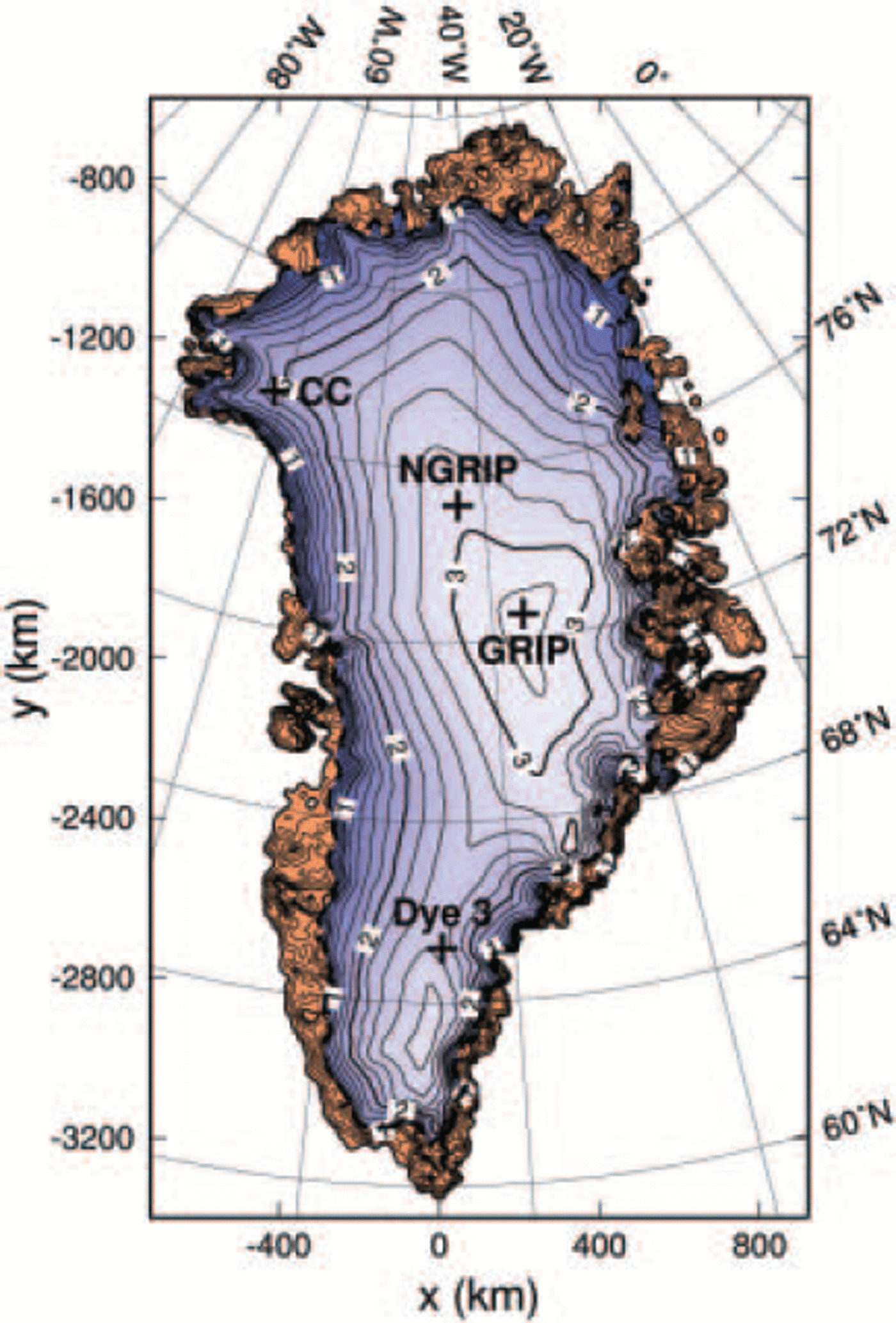
The Greenland ice sheet is the second-largest present-day ice mass on Earth. While its surface (Fig. 1) and basal topographies are known very accurately (Reference Bamber, Ekholm and KrabillBamber and others, 2001a,Reference Bamber, Layberry and Goginenib, Reference Bamber, Layberry and Goginenic), and surface velocity measurements are available all around the 2000 m elevation contour (Reference Thomas, Csathó, Gogineni, Jezek and KuivinenThomas and others 1998; see also nsidc.org/data/parca) and at several other locations, direct information on the thermodynamic state of the ice sheet is limited to a small number of deep ice cores. For the past, apart from limited data on ice extent since the Last Glacial Maximum (LGM) at approximately 21 kyr BP, information on the dynamics and thermodynamics of the Greenland ice sheet can only be obtained from flow models.

Fig. 1.

Surface topography of the Greenland ice sheet, by Reference Bamber, Layberry and GogineniBamber and others (2001b, c). Contour spacing is 200 m; labels are in km a.s.l. The GRIP, NorthGRIP (NGRIP), Camp Century (CC) and Dye 3 ice-core locations are indicated. Brown areas mark ice-free land.

A number of studies on the Greenland ice sheet over the last glacial–interglacial cycles have been conducted with three-dimensional thermomechanical ice-sheet models (Reference Letréguilly, Reeh and HuybrechtsLetréguilly and others, 1991; Reference Calov and HutterCalov and Hutter, 1996; Reference Ritz, Fabre and LetréguillyRitz and others, 1997; Reference Greve, Weis and HutterGreve and others, 1998, Reference Greve, Mügge, Baral, Albrecht, Savvin, Hutter, Wang and Beer1999; Reference Van de WalVan de Wal, 1999; Reference Marshall and CuffeyMarshall and Cuffey, 2000; Reference HuybrechtsHuybrechts, 2002; Reference Tarasov and PeltierTarasov and Peltier, 2003). These models have in common that they solve the equations of the shallow-ice approximation (Reference HutterHutter, 1983; Reference MorlandMorland, 1984). Climate forcing is provided based on the present distributions of precipitation/accumulation and surface history, modified by time-dependent offsets derived from ice-core isotope records (δ¹⁸O, δD). Except for the study by Reference Tarasov and PeltierTarasov and Peltier (2003), the geothermal heat flux, which enters the ice body from below and provides the lower boundary condition for the temperature field in the ice, is assumed to be spatially and temporally constant, with values in the range 42– 65 mWm–2. As demonstrated by Reference Greve and HutterGreve and Hutter (1995), this input quantity plays a crucial role for the modelled basal temperature, surface topography and ice-flow velocities, and deserves further attention.

Therefore, in this study we attempt to constrain the spatial distribution of the geothermal heat flux with the available temperature data of four deep ice cores: the Greenland Icecore Project (GRIP), North Greenland Icecore Project (NorthGRIP), Camp Century and Dye 3 cores (Fig. 1). In section 2, the main features of the thermomechanical ice-sheet model SICOPOLIS are described. In section 3, a climatic forcing for the last glacial–interglacial cycles is introduced, which goes beyond previous approaches by interpolating the precipitation and surface-temperature patterns between present conditions and LGM anomalies provided by a general circulation model (GCM). Section 4 describes the general set-up of transient simulations from 250kyr BP until today covering two entire glacial-interglacial cycles. In section 5, four simulations with different assumptions for the geothermal heat flux are discussed. It is demonstrated that with a pattern, based on the global heat-flow representation by Reference Pollack, Hurter and JohnsonPollack and others (1993) and modified with suitable values at the ice-core locations mentioned above, the basal temperatures can be matched accurately.

2. Thermomechanical Ice-Sheet Model Sicopolis

The model SICOPOLIS (SImulation COde for POLythermal Ice Sheets) simulates the large-scale dynamics and thermodynamics (ice extent, thickness, velocity, temperature, water content and age) of ice sheets three-dimensionally and as a function of time (Reference GreveGreve, 1997). It is based on the shallow-ice approximation (Reference HutterHutter, 1983; Reference MorlandMorland, 1984) and the rheology of an incompressible, heat-conducting, power-law fluid (Glen’s flow law; see Reference PatersonPaterson, 1994). The thermomechanical coupling is described by the temperature- and water-content-dependent rate factor in the form of Reference Greve, Weis and HutterGreve and others (1998) which follows Reference PatersonPaterson’s (1994) recommendations. Isostatic depression and rebound of the lithosphere due to changing ice load is modelled by the local-lithosphere-relaxing-asthenosphere (LLRA) approach with an isostatic time lag τiso (Reference Le Meur and HuybrechtsLe Meur and Huybrechts, 1996; Reference Greve, Straughan, Greve, Ehrentraut and WangGreve, 2001).

A particular feature of the model thermodynamics is the distinction between cold ice with a temperature below the pressure-melting point and temperate ice with a temperature at the pressure-melting point. The interface that separates cold and temperate ice is monitored using Stefan-type energy-flux and mass-flux matching conditions. In the cold ice, which makes up by far the larger part of the volume of an ice sheet, the temperature evolution is computed from the three-dimensional energy balance which includes horizontal and vertical advection, vertical heat conduction and dissipative strain heating. By contrast, in the temperate ice, which can exist as thin layers overlying a temperate base, the energy balance provides an evolution equation for the water content which comprises horizontal and vertical advection, melting due to dissipation and downward water drainage. The thermal inertia of the lithosphere is accounted for by solving the vertical heat-conduction equation in a 5 km thick thermal boundary layer below the ice. The set of evolution equations is listed in the study by Reference Greve, Weis and HutterGreve and others (1998).

Basal sliding is described by a Weertman-type sliding law in the form of Reference Greve, Weis and HutterGreve and others (1998), modified to allow for sub-melt sliding as proposed by Reference Hindmarsh and Le MeurHindmarsh and Le Meur (2001):

(1)

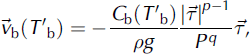
where is the basal-sliding velocity, the basal shear traction in the bed plane, ρ the ice density, g the gravity acceleration and ρ = ρgH the overburden pressure. The stress and pressure exponents are chosen as p = 3 and q = 2. The sliding coefficient C _b depends on the homologous temperature T’b (temperature relative to pressure melting, in °C) via

(2)

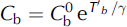
(note that T′_b ≤ 0°C) where 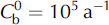is the sliding coefficient at the pressure-melting point, and the constant 7 is set to γ = 1°C. In case of a temperate base (T′_b ≤ 0°C). basal melting is computed by balancing the heat fluxes from the ice and the lithosphere and the heat production due to basal sliding .

External forcing is specified by (i) the mean annual air temperature at the ice surface, (ii) the surface mass balance (accumulation, ablation), (iii) the global sea level which defines the land area available for glaciation, and (iv) the geothermal heat flux prescribed at the bottom of the lithospheric thermal boundary layer. All computations are carried out in a stereographic plane with standard parallel at 71 ˚N, spanned by the Cartesian coordinates x and y. The vertical coordinate z is taken positive upward, and the zero level is the present-day reference geoid. The distortions due to the stereographic projection are corrected by appropriate metric coefficients.

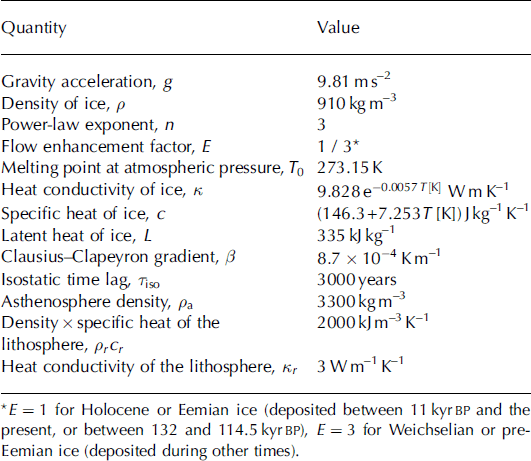
The standard values of the relevant physical parameters used for the simulations herein are listed in Table 1.

Table 1.

Standard physical parameters of the ice-sheet model SICOPOLIS

3. Climatic Forcing

As measure for the climate state at any time t, a glacial index g(t) is defined such that g = 1 denotes LGM conditions and g = 0 present conditions (Reference Forsström, Sallasmaa, Greve and ZwingerForsström and others, 2003; Reference Forsström and GreveForsström and Greve, 2004). It is based on the GRIP surface temperature (T _s) history derived from the δ¹⁸O record (Reference DansgaardDansgaard and others, 1993) with the quadratic conversion formula found by Reference Johnsen, Dahl-Jensen, Dansgaard and GundestrupJohnsen and others (1995),

(3)

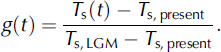
The reference values are T _s,present = -31.74°C (for δ¹⁸O = -35.2‰) and T _s,LGM = -55.15°C (for δ¹⁸O = -42.71 ‰), where the latter represents the LGM minimum taken at 21.9 kyr BP.

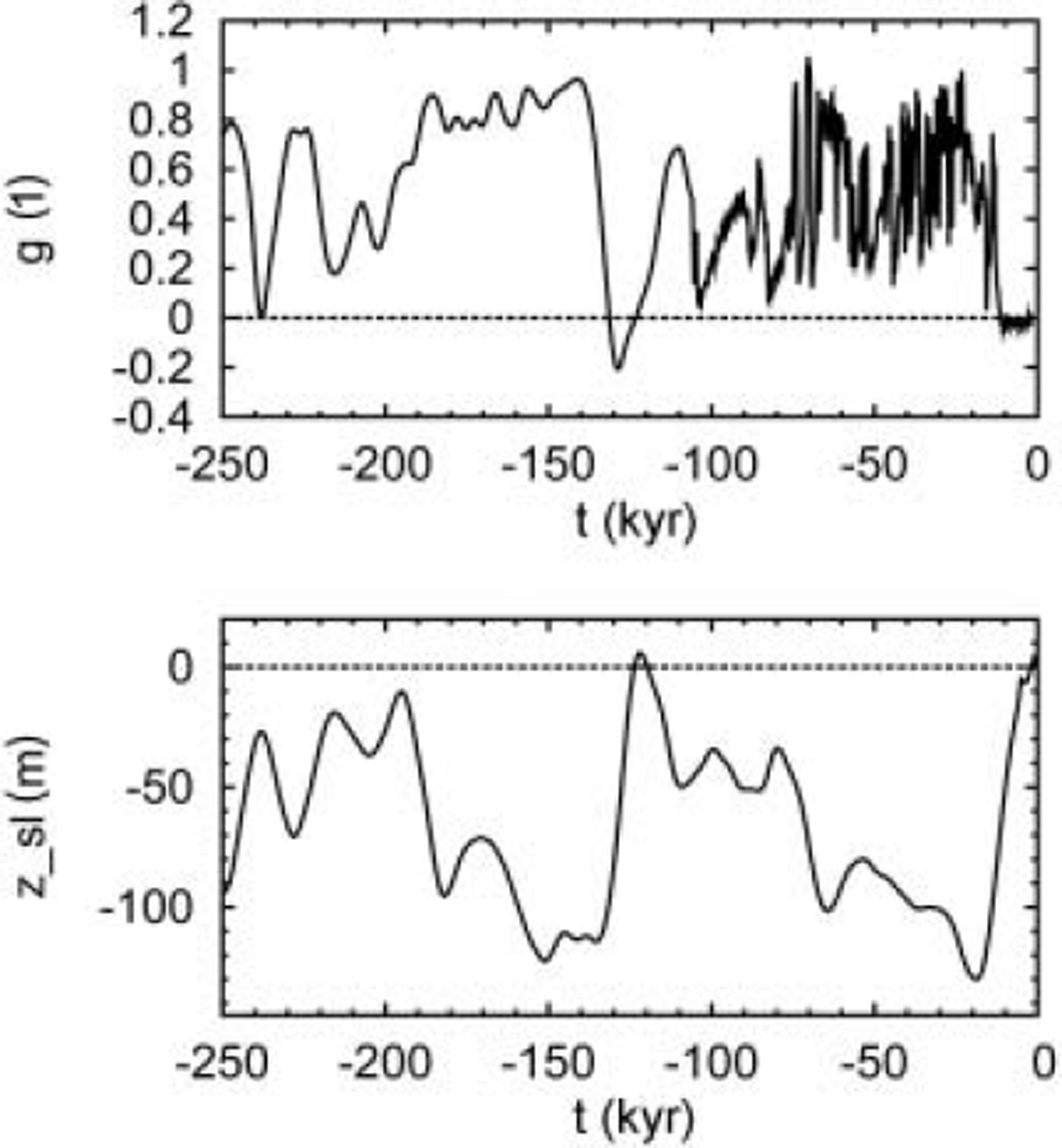
Prior to 105kyr BP, the GRIP record is believed to be falsified due to ice-flow irregularities (North Greenland Ice Core Project members, 2004), and for that period the glacial index is derived from the surface-temperature history based on the δD record of the Antarctic Vostok ice core (Reference PetitPetit and others, 1999) instead. In order to smooth out rapid climate oscillations which are unlikely to be in phase between Greenland and Antarctica, the Vostok record is subjected to a Gaussian filter with 2 kyr filter width. The resulting glacial index is shown in Figure 2a for the period from 250 kyr BP until today. Similar synthetic blends of these two ice-core records have been used by Reference Marshall and CuffeyMarshall and Cuffey (2000) and Reference HuybrechtsHuybrechts (2002).

Fig. 2.

(a) Glacial index g(t) derived from the GRIP and Vostok surface temperature records (Reference DansgaardDansgaard and others, 1993; Reference Johnsen, Dahl-Jensen, Dansgaard and GundestrupJohnsen and others, 1995; Reference PetitPetit and others, 1999). (b) Sea-level history z _sl(t) derived from the SPECMAP marine δ¹⁸O record (Reference Imbrie, Berger, Imbrie, Hays, Kukla and SaltzmanImbrie and others, 1984).

This glacial index is used to determine the surface-temperature and precipitation distribution over the ice sheet by interpolating between present and LGM conditions. The present-day surface air temperature is parameterized as a function of surface elevation, h, and latitude, φ, following Reference Ritz, Fabre and LetréguillyRitz and others (1997):

(4)

where T _ma and T_mj are the mean annual and mean July (summer) surface temperatures, respectively, and the lapse rates are γ_ma = -7.992°C km−1 and γ_mj = -6.277°C km−1. The present precipitation map, P _ma, present (λ, φ) (the index ‘ma’ stands for ‘mean annual’, λ denotes longitude and φ latitude), is constructed based on the digitized accumulation map by Calanca and others (2000), complemented by Reference JaegerJaeger’s (1976) global precipitation map in the regions not covered by the Calanca and others (2000) data.

For the LGM counterparts of these climatic input fields, results of GCM simulations with the UKMO model (Reference Hewitt and MitchellHewitt and Mitchell 1997), carried out for the Paleoclimate Modelling Intercomparison Project (PMIP; see www-lsce.cea.fr/pmip), are utilized. The coarse model output (2.5˚ long. × 2.5˚ lat.) is interpolated to the finer SICOPOLIS grid with inverse-distance weighing. In order to largely eliminate systematic errors of these simulations, anomalies with respect to present-day conditions (denoted by the hat symbols) are defined,

(5)

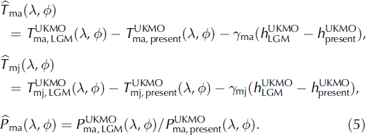
Note that the temperature anomalies are differences, whereas the precipitation anomaly is defined as a ratio. In the former, the contribution due to orographic differences between the LGM ice sheet and the present-day ice sheet is eliminated by the lapse-rate terms. In order to adjust the anomalies to data of the LGM climate, the anomalies are further modified by factors ft_ma, ftmj and f_{p ma} :

(6)

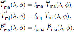
The factors are chosen as ft_ma = ftmj = 1 :9 and f _pma = 1. The temperature factors increase the LGM anomaly of the mean annual surface temperature at GRIP from -12.4°C to -23.4°C, in agreement with the palaeotemperatures derived by Reference Johnsen, Dahl-Jensen, Dansgaard and GundestrupJohnsen and others (1995). The precipitation anomalies at the GRIP, NorthGRIP, Camp Century and Dye 3 ice-core locations are within the range of 0.228 (NorthGRIP) and 0.294 (GRIP), which is consistent with other estimates (Reference Johnsen, Dahl-Jensen, Dansgaard and GundestrupJohnsen and others, 1995; Reference Cuffey and ClowCuffey and Clow, 1997; Reference Dahl-Jensen, Gundestrup, Gogineni and MillerDahl-Jensen and others, 2003), so that a modification is not required.

With the above-defined glacial index, the mean annual surface temperature is parameterized by

(7)

accordingly for the mean July surface temperature Tmj (λ, φ, t), and the mean annual precipitation rate is computed as

(8)

Equations (7) and (8) produce present-day conditions for g=0 and LGM conditions for g=1 as required. The exponential precipitation interpolation of Equation (8) was chosen because it also fulfils the condition P _ma(g → ∞) = 0 (note that ln because 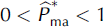), in other words, the precipitation vanishes at the limit of extremely cold conditions.

Conversion from mean annual precipitation P _ma to snowfall (solid precipitation) is done on a monthly basis with the empirical relation by Reference MarsiatMarsiat (1994),

(9)

where S _mm is the mean monthly snowfall and T _mm the mean monthly surface temperature computed from T _ma and T_mj by assuming a sinusoidal annual cycle. Mean monthly rainfall (liquid precipitation) is obtained as the difference between precipitation and snowfall.

Surface melting is parameterized by Reference ReehReeh’s (1991) degree-day method, supplemented by explicit consideration of rainfall and the semi-analytical solution for the positive-degree-day integral by Reference Calov and GreveCalov and Greve (2004). Following Reference Tarasov and PeltierTarasov and Peltier (2002), different degree-day factors for ice melt and snowmelt and for warm and cold conditions are introduced. South of 72° N, it is assumed that warm conditions prevail, so that

(10)

North of 72° N, the actual degree-day factors are made dependent on the mean July surface temperature T _mj,

(11)

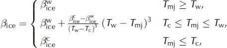
and

(12)

For the limiting temperatures, the values by Reference Tarasov and PeltierTarasov and Peltier (2002), T _w = 10°C and T _c = -1°C, are applied, and the limiting degree-day factors are chosen as and . Further, according to Reference ReehReeh (1991), the saturation factor for the formation of superimposed ice is chosen as P _max = 0.6, and the standard deviation of short-term, statistical air-temperature fluctuations is set to σ_stat = 4.5°C.

Sea-level forcing z_sl, which determines the land area available for glaciation, is derived from the SPECMAP (spectral-mapping project) marine δ¹⁸O record (Reference Imbrie, Berger, Imbrie, Hays, Kukla and SaltzmanImbrie and others, 1984) converted to global sea level by

(13)

This parameterization produces an LGM sea-level minimum of −130 m at 19 kyr BP and an Eemian sea-level high of 5.9 m at 122 kyr BP (see Fig. 2b).

4. Simulation Set-Up

The model domain covers the entire land area of Greenland and the surrounding sea, projected to a polar stereographic map with standard parallel at 71˚ N and central meridian at 44˚ W. Distortions due to this projection are accounted for as metric coefficients in the model equations. Present geometry (surface elevation, bedrock elevation, ice thickness, equilibrated bedrock elevation) is taken from the 5 km dataset by Reference Bamber, Layberry and GogineniBamber and others (2001b, c).

All input data have been resampled to a 20 km grid, which leads to 82 by 140 gridpoints in the stereographic plane. In the vertical, a coordinates are used, in that the cold-ice column, the temperate-ice layer (if present) and the lithosphere layer are mapped separately to [0,1] intervals. The cold-ice column is then discretized by 81 gridpoints (which densify towards the base), and the temperate-ice and lithosphere layers are each discretized by 11 equidistant gridpoints.

Model time for all simulations is from 250 kyr BP until today. Initial conditions are provided by spin-up simulations from 422 kyr BP until 250 kyr BP with a quasi-steady-state lithosphere temperature (that is, its vertical gradient is balanced by the geothermal heat flux without any time lag); in other words, the thermal inertia of the lithosphere is switched off during spin-up. The time-step for all model components is 5 years. With these settings, a full simulation (spin-up run and transient run) requires approximately 11 hours CPU time on a 3.4GHz Pentium-4 PC operated under LINUX.

5. Simulations With Varied Geothermal Heat Flux

5.1. Run hf_cst: constant heat flux

The starting point of this study is the assumption of a spatially constant geothermal heat flux of 60 mWm–², which was obtained by matching measured and simulated basal temperatures at GRIP. This value is within the range of the heat fluxes used in previous modelling studies of the Greenland ice sheet (see section 1), and slightly larger than the heat fluxes inferred for the GRIP location by Reference Dahl-JensenDahl-Jensen and others (1998) and Reference Tarasov and PeltierTarasov and Peltier (2003). Simulation hf_cst has been run with this value, and the results for the ice thicknesses and basal temperatures for the GRIP, NorthGRIP, Camp Century and Dye 3 ice-core locations are listed in Table 2.

Table 2.

Simulated and observed ice thicknesses and basal temperatures for the GRIP, NorthGRIP, Camp Century and Dye 3 ice-core locations

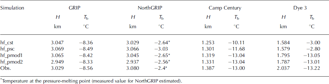
For GRIP, the remaining misfit of the basal temperature is only 0.2°C, and the adequate choice of the geothermal heat flux is validated by the excellent agreement for the ice thickness (18m or 0.6% misfit). Also, at NorthGRIP good agreement is achieved; the simulated and observed basal temperatures are both at the pressure-melting point, and the ice column is 51 m (1.7%) too thin. This good agreement is surprising, because even in the recent study by Reference Tarasov and PeltierTarasov and Peltier (2003) where a very thorough tuning procedure of a similar model was carried out, the basal temperature at NorthGRIP was still 5°C below pressure melting. Therefore, the improved representation of the conditions at NorthGRIP in this study is due to the more detailed climatic forcing (section 3), which accounts for the variability of the spatial distribution of precipitation and surface temperature over time. At Camp Century, the simulated temperature is 2.9°C too high, and the ice column is 134 m (9.7%) too thin. This indicates that the geothermal heat flux is too large. Dye 3 exhibits the largest disagreement, with a 10.2°C too high temperature and a 453 m (22.2%) too thin ice column. This poor agreement, already reported in previous studies (e.g. Reference HuybrechtsHuybrechts, 1996), suggests a distinctly lower geothermal heat flux in the southern part of the Greenland ice sheet.

5.2. Run hf_psc: scaled Pollack and others (1993) heat flux

The above assumption of a spatially constant geothermal heat flux is very unlikely for an area as large as Greenland. The spherical harmonic representation to degree and order 12 of the global heat flow by Reference Pollack, Hurter and JohnsonPollack and others (1993) shows a significant horizontal gradient (∼25mWm^-2 per 1000 km) mainly towards the east in the Greenland area. However, the representation is poorly constrained in this region because of the small number of local supporting data, and as already pointed out by Reference Tarasov and PeltierTarasov and Peltier (2003), the heat fluxes are generally too large to provide realistic basal temperatures. Therefore, simulation hf_psc has been run with the heat-flux distribution by Reference Pollack, Hurter and JohnsonPollack and others (1993), scaled by a constant factor such that the geothermal heat flux at GRIP is reduced to the value 60 mWm^–2 of run hf_cst. The resulting heat-flux map is shown in Figure 3. Results for the four ice-core locations are summarized in Table 2.

Fig. 3.

Distribution of the geothermal heat flux by Reference Pollack, Hurter and JohnsonPollack and others (1993) scaled to a value of 60 mW m^–2 at GRIP (for simulation hf_psc). The heavy dashed line indicates the present-day ice margin.

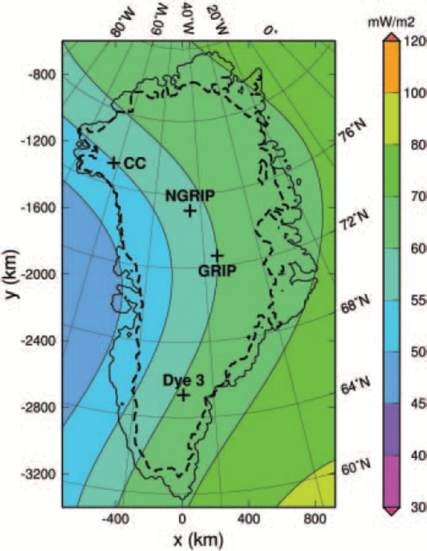
The agreement with observations has not changed significantly compared to simulation hf_cst. It is still excellent at GRIP, not surprisingly since the geothermal heat flux has not been changed at this site. For NorthGRIP, the ice thickness fits slightly better and the temperature slightly worse, which indicates that the remaining misfit is not attributable to the geothermal heat flux alone. The agreement at Camp Century has improved distinctly for both the ice thickness and the basal temperature, which is a clear consequence of the reduced geothermal heat flux in the area. For Dye 3, the results are very similar to those of simulation hf_cst, so that the large misfit remains.

5.3. Runs hf_pmod1/2: modified Pollack and others (1993) heat flux

To achieve better agreement between measured and modelled basal temperatures and ice thicknesses, the above-constructed geothermal-heat-flux map is modified as follows. For the N _m = 444 margin points of the numerical domain, (x_n,y_n), n = 1…N _m, the geothermal heat fluxes q _g eo, n of the above procedure are kept. For the N_c = 4 ice-core locations (xn,y_n), n = N_m + 1 … N _m + N_c (GRIP, NorthGRIP, Camp Century, Dye 3), the geothermal heat fluxes q _geo,n are chosen such that the simulated basal temperatures match the modelled ones. With these N = N_m + N_c = 448 reference points, the new geothermal-heat-flux distribution q _geo(x, y) is computed by the weighed interpolation

(14)

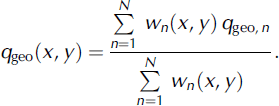
The weighing factors w_n are n=taken 1 as the squares of the inverse distances from the arbitrary position (x, y) to the reference points (x_n ,y_n ),

(15)

The additional factors 1/N _m and 1/N _c, respectively, have been introduced in order to provide a balance between the influence of the large number of margin points and the small number of ice-core locations.

The basal melting conditions at NorthGRIP make the matching procedure of basal temperatures non-unique there. Only the minimum heat flux required to produce pressure melting is well defined; any further increase leads merely to increased basal melting. Therefore, two different matching procedures are carried out, (i) with the minimum heat flux at NorthGRIP, and (ii) with the heat flux that produces the basal melting rate of 77 mm ice equiv. a^-1 reported by Reference Dahl-Jensen, Gundestrup, Gogineni and MillerDahl-Jensen and others (2003). This yields the following set of values (left/right values correspond to procedures (i) and (ii), respectively):

(16)

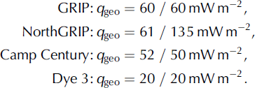
Figure 4 depicts the modified maps of the geothermal heat flux. The influence of the very different heat fluxes at NorthGRIP is most pronounced in the northeastern sector of Greenland. Table 2 displays the results of the corresponding simulations hf_pmod1 (procedure (i)) and hf_pmod2 (procedure (ii)) for the four ice-core locations.

Fig. 4.

Distributions of the geothermal heat flux based on Reference Pollack, Hurter and JohnsonPollack and others (1993), modified with the values of Equation (16) for GRIP, NorthGRIP, Camp Century and Dye 3, for simulations hf_pmod1 (left) and hf_pmod2 (right). The heavy dashed lines indicate the present-day ice margin.

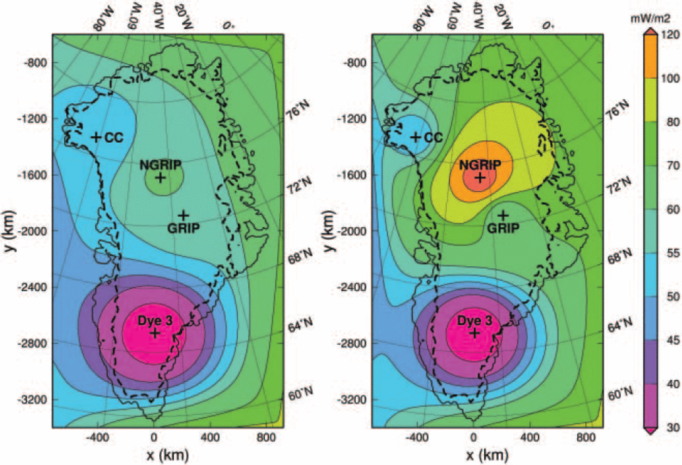
Evidently, for both simulations the basal temperatures at the four ice-core locations are matched within ∼0.2°C. For simulation hf_pmod1, the resulting ice thicknesses are 1.2% too large at GRIP, 1.1% too small at NorthGRIP, 4.9% too small at Camp Century and 11.9% too small at Dye 3. By contrast, for simulation hf_pmod2 all thicknesses are too small, at GRIP by 2.6%, at NorthGRIP by 4.6%, at Camp Century by 4.0% and at Dye 3 by 12.3%. However, Figure 5, which displays the simulated surface topography and the ice-thickness misfit for run hf_pmod2, shows that this is not a systematic misfit: in other regions of the ice sheet the simulated thicknesses are too large. Since the heat flux at NorthGRIP used for simulation hf_pmod2 also produces a close match of the simulated basal melting rate (7.06 mm ice equiv. a^-1) to the above-mentioned estimate by Reference Dahl-Jensen, Gundestrup, Gogineni and MillerDahl-Jensen and others (2003) and North Greenland Ice Core Project members (2004) (whereas it is <0.1 mm ice equiv. a^-1 for simulation hf_pmod1), we consider simulation hf_pmod2 (and the corresponding heat-flux distribution of Figure 4, right panel) as more realistic and limit the following discussion to it.

Fig. 5.

Simulation hf_pmod2: present-day surface topography (left panel; contour spacing 200 m, labels in km a.s.l.), and difference between simulated and observed present-day ice thickness (right panel). The heavy dashed lines indicate the simulated (left panel) and observed (right panel) ice margins.

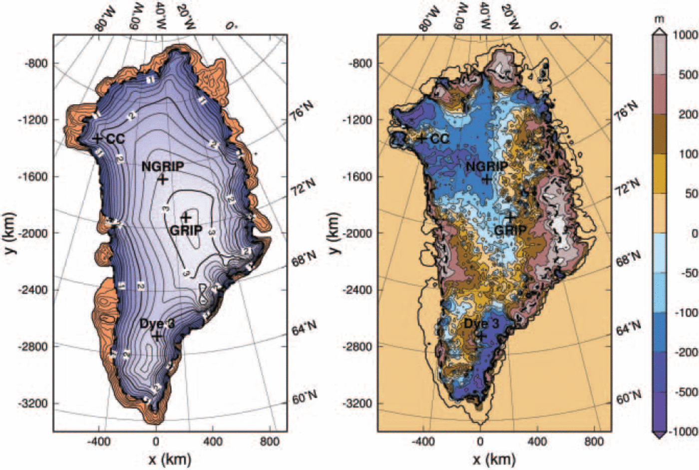
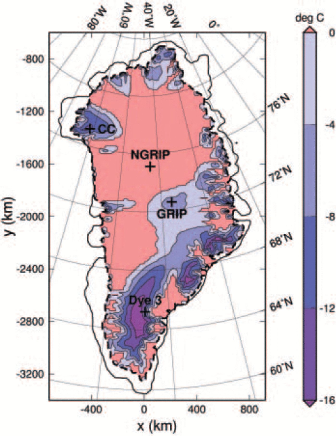
Figure 6 shows the homologous basal temperature computed with simulation hf_pmod2. The large geothermal heat fluxes around NorthGRIP and in the entire northeastern sector of the ice sheet lead to widespread pressure-melting conditions at the ice base. Basal melting also prevails in West Greenland in a wide flowband upstream of Jakobshavn Isbræ where the heat fluxes are lower. Naturally, the anomaly of very low heat fluxes around Dye 3 entails low basal temperatures in the central part of south Greenland.

Fig. 6.

Simulation hf_pmod2: present-day basal homologous temperature (temperature relative to pressure melting). Red areas are at the pressure-melting point. The heavy dashed line indicates the simulated ice margin.

The small value of 20 mWm–² for the geothermal heat flux at Dye 3 found here (Equation (16)) is corroborated by the temperature profile published in Reference Dahl-JensenDahl-Jensen and others (1998) (the gradient at the base corresponds to a heat flow of ∼25mWm–² into the ice body) and the findings by Reference HuybrechtsHuybrechts (1996) who reports that in his reference run 0.44 HFU (heat-flow units) = 18.5 mWm–² are required to match the observed basal temperature. However, Figure 5 shows that the south dome of the ice sheet is situated too far west, and that the eastern part of the ice sheet south of 67° N is generally too thin by 200-500m. This explains the significant ice-thickness misfit at Dye 3. The discrepancy is likely due to too low precipitation rates over the southeastern ice sheet.

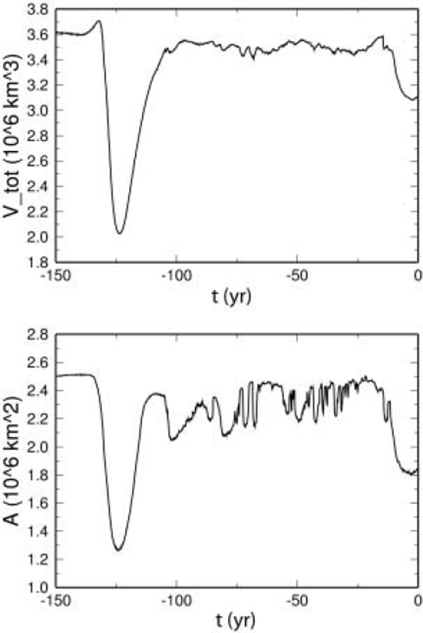
Figure 7 shows the evolution of the ice volume and the ice-covered area over the last 150 kyr. As expected, both quantities are larger during glacial and smaller during interglacial periods, and the Eemian ice retreat is much more pronounced than the retreat during the Holocene. The simulated Eemian ice-volume minimum at 123.5 kyr BP (2.026 × 106km ) corresponds to an equivalent sea-level rise of 2.75 m compared to the simulated present-day volume (3.115 × 10⁶ km ). The LGM ice volume at 21 kyr BP is 3.487 × 106km³ or 0.94 m of sea-level lowering. Note that values for sea-level equivalents are based on the ratio 7.2/2.85 = 2.5263 ms.l.e: per 106km³ ice volume, which was reported for the Greenland ice sheet by Reference Church and HoughtonChurch and others (2001, table 11.3).

Fig. 7.

Simulation hf_pmod2: evolution of the ice volume V ^tot and the ice-covered area A over the last 150 kyr.

The sea-level equivalent of the simulated present-day ice volume is 7.87 m, 6.2% more than the 7.41m which correspond to the observed volume of 2.932 × 10⁶ km . As can be inferred from Figure 5 (right panel), most of this difference originates from simulated ice cover in areas where there is no ice in reality. In Peary Land, north of 82˚ N, the simulation predicts an ice tongue which has no real counterpart, and similarly the almost ice-free area east of 30˚ W, between 68˚ N and 74˚ N, remains glacierized in the simulation result. These deficiencies are most likely due to inaccuracies in the mass-balance forcing.

6. Conclusion

The thermomechanical ice-sheet model SICOPOLIS was applied to the Greenland ice sheet, and simulations were carried out over two glacial–interglacial cycles, driven by a climatic forcing interpolated between present conditions and LGM anomalies on the basis of a glacial index derived from the GRIP δ¹⁸O and the Vostok δD record. Four different distributions of the geothermal heat flux were employed: a constant value for the entire ice sheet, a scaled Reference Pollack, Hurter and JohnsonPollack and others (1993) heat-flux distribution, and two different heat-flux maps assembled by modifying the latter with prescribed values for the GRIP, NorthGRIP, Camp Century and Dye 3 ice-core locations.

It was demonstrated that with the modified Reference Pollack, Hurter and JohnsonPollack and others (1993) map shown in Figure 4 (right panel) an excellent match is achieved for the basal temperatures of the four ice cores, including the estimated basal melting rate at NorthGRIP. This heat-flux map still shows the increasing trend from west to east of the original Reference Pollack, Hurter and JohnsonPollack and others (1993) distribution. The most prominent overlying structures are the high-heat-flux anomaly around NorthGRIP with values up to 135 mWm–² , and the low-heat-flux anomaly around Dye 3 with values down to 20 mWm–² . However, since the interpolation of the geothermal heat flux in the interior of Greenland is only based on the four boreholes, it is very likely that the spatial variation is much larger in reality. This notion is supported by Reference Fahnestock, Abdalati, Joughin, Brozena and GogineniFahnestock and others (2001), who used data from airborne ice-penetrating radar and inferred highly varying basal melting rates in the northeastern sector of the Greenland ice sheet which correspond to local heat fluxes as high as 15-30 times average values.

The ice thickness, which was used for validating the simulation results, shows a good agreement for GRIP, NorthGRIP and Camp Century, but there is a significant misfit of > 12% for Dye 3 which originates from a shift of the simulated with respect to the observed south dome. This discrepancy, other inaccuracies of the simulated ice thickness and the failure of the simulation to reproduce the observed ice margin in the far north and in parts of East Greenland, are most likely due to the above-mentioned further variability of the geothermal heat flux as well as deficiencies of the input precipitation rate. Therefore, the importance for improving the mass-balance input is underlined. In future work, alternative precipitation data like the map assembled as part of the PARCA (Program for Arctic Regional Climate Assessment) project (Reference Bales, McConnell, Mosley-Thompson and CsathóBales and others, 2001) will be considered. It may also be helpful to compare the output of different GCM simulations for defining LGM anomalies. However, in the long term the most promising approach is to overcome the problem of mass-balance input by conducting coupled simulations with atmosphere and ice-sheet models.