Problem formulation of SOMIs

The frequency response of an ideal SOI is given by

(1)$$H(\,j{\omega})= {\displaystyle{1} \over {{\omega}^2},$$

where ω represents the angular frequency in radians per second. Since the magnitude response of an open-circuited stub decreases with frequency, an open-circuited stub can be chosen to design an integrator. Its chain scattering matrix is given by [Reference Hsue, Tsai and Kan8]

(2)$$\eqalign{\left[ A \right] & = \left[ {\matrix{ {T_{11}} & {T_{12}} \cr {T_{21}} & {T_{22}} \cr } } \right] \cr & = \displaystyle{1 \over {(1 + z^{-1})}}\left[ {\matrix{ {(1 + \kappa ) + (1-\kappa )z^{-1}} & {\left( {\kappa -\kappa z^{-1}} \right)} \cr {-\kappa + \kappa z^{-1}} & {(1-\kappa ) + (1 + \kappa )z^{-1}} \cr } } \right], \cr & } $$

and S ₂₁ is given by

(3)$$S_{21} = {\displaystyle{1} \over {T_{11}}} = {\displaystyle{1+z^{-1}} \over {(1 + \kappa) + (1 - \kappa)z^{-1}}},$$

where z = e ^jβl in which β represents the phase constant, l represents the physical length of the line element, and the coefficient κ is given by

(4)$$ {{\kappa = \displaystyle{Z_{0}} \over {2 \times Z_{oc} }}, $$

where Z ₀ represents the reference impedance, that is 50 Ω and Z _oc is the characteristic impedance of an open-circuited stub. Serial line sections shunted with open circuited stub should be employed in the transmission line configuration to design an integrator by cascading. A cascaded connection of two-port network is equivalent to a single two-port network containing a product of the two matrices. The chain scattering matrix of transmission line section is given by [Reference Hsue, Tsai and Kan8].

The chain scattering matrix for transmission line section in Z domain is given by [Reference Hsue, Tsai and Kan8]

(5)$$\eqalign{\left[ B \right] & = \left[ {\matrix{ {T_{11}} & {T_{12}} \cr {T_{21}} & {T_{22}} \cr } } \right] \cr & = \displaystyle{1 \over {z^{-1/2}(1-\Gamma ^2)}}\left[ {\matrix{ {1-\Gamma ^2z^{-1}} & {\left( {-\Gamma -\Gamma z^{-1}} \right)} \cr {1-\Gamma z^{-1}} & {-\Gamma ^2 + z^{-1}} \cr } } \right],} $$

where the reflection coefficient Γ is given by

(6)$$\Gamma = { \displaystyle{Z_{TL}-Z_{0}} \over {Z_{TL}+Z_{0}} },$$

where Z _TL represents the characteristic impedance of serial transmission line section. The chain scattering matrix of a short-circuited stub is given by [Reference Tsai and Wu10]

(7)$$\left[ C \right] = \displaystyle{1 \over {1-z^{-1}}}\left[ {\matrix{ {(1 + \delta )-(1-\delta )z^{-1}} & {\delta + \delta z^{-1}} \cr {-\delta -\delta z^{-1}{\rm }} & {(1-\delta )-(1 + \delta )z^{-1}} \cr } } \right],$$

where the coefficient δ is given by

(8)$$\delta = { \displaystyle{Z_{0}} \over {2 \times Z_{sc}} }, $$

where Z _sc represents the characteristic impedance of the short-circuited stub.

Assume the SOI is composed of P open-circuited stubs, Q short-circuited stubs, and R transmission line sections. The overall S ₂₁ in generalized is given by

(9)$$\eqalign{S_{21} &= \displaystyle{1 \over {T_{11}}} \cr & = \displaystyle{{{(1 + z^{-1})}^P{(1-z^{-1})}^Qz^{-R/2}\prod\nolimits_{r = 1}^R {(1-\Gamma _r^2 )} } \over {\alpha _0 + \alpha _1z^{-1} + \alpha _2z^{-2} + \alpha _3z^{-3} + \cdots + \alpha _Nz^{-N}}},} $$

where, P denotes the number of open-circuited stubs, Q denotes the number of short-circuited stubs, R denotes the number of transmission line section, N is the total number of line elements N = P + Q + R and $\alpha _{0},\alpha _{1},\alpha _{2}, {\ldots }, \alpha _{N}$ coefficients are functions of reflection coefficient of each transmission line sections and characteristic impedances of stubs (in terms of coefficient κ of open-circuited stub and coefficient δ of short-circuited stub). Furthermore, serial transmission lines shunted with stubs may be employed to design the SOMI. Then frequency-domain response of the transfer function is thus obtained which has the characteristic of an integrator. The following two approaches have been used to design a wideband SOMI.

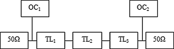
Approach-I: In this approach, we may select two open-circuited stubs and three transmission line sections as shown in Fig. 1(a), where P = 2, R = 3. Overall S ₂₁ of the proposed-1 SOMI is given by

(10)$$S_{21} = {{\displaystyle{(1+z^{-1})^2 z^{-3/2}\prod\nolimits_{r=1}^3 (1-\Gamma_r^2)} \over {\alpha_{0}+\alpha_{1}z^{-1}+\alpha_{2}z^{-2}+\alpha_{3}z^{-3}+\alpha_{4}z^{-4}+\alpha_{5}z^{-5}} }.$$

Fig. 1.

Configuration of the proposed-1 SOMI.

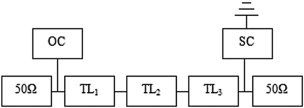
Approach-II: In this approach, a short-circuited stub is cascaded with the transmission line sections and an open-circuited stub as shown in Fig. 1(b), where P = 1, Q = 1, R = 3. Overall S ₂₁ of the proposed-2 SOMI is given by

(11)$$S_{21}= {{ \displaystyle{(1-z^{-2})z^{-3/2}\prod\nolimits_{r=1}^3 (1-\Gamma_r^2)} \over {\alpha_{0}+\alpha_{1}z^{-1}+\alpha_{2}z^{-2}+\alpha_{3}z^{-3}+\alpha_{4}z^{-4}+\alpha_{5}z^{-5}} }}.$$

The term (1 + z ⁻¹) is due to open-circuited stub, the term (1 − z ⁻¹) is due to short-circuited stub, and z ^−3/2 is a delay factor of transmission line section. These line elements are equal length transmission lines having length l = λ₀/4 at operating frequency 12.5 GHz.

Next, the task is to obtain the optimum value of characteristic impedances of line elements for the proposed-1 and proposed-2 SOMI. These characteristic impedances of line elements are obtained by using optimization algorithm. The design of SOMI is taken into consideration, as an approximation problem, where the cost function is to be lessened. The cost function is the difference between the magnitude response of an ideal SOI and the designed SOMI. The cost function is formulated in the least squares sense and can be expressed as

(12)$$ CF = min \int \limits_0^\pi \vert {E(\omega) \vert ^2}\ d {\omega}=min\int\limits_0^\pi \vert H({\omega})-S_{21} \vert ^2\ d{\omega},$$

where E(ω) = (H(ω) − S ₂₁) is the cost function, in which H(ω) is the frequency response of an ideal SOI.

Employed methodologies

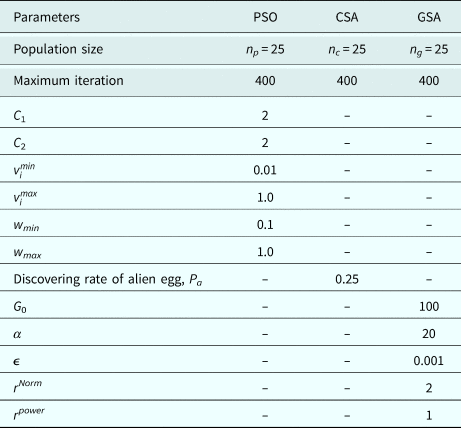
In this section, three population-based heuristic search algorithms namely PSO, CSA, and GSA are used to minimize the cost function to find the optimal values of characteristic impedances of line elements for designed wideband SOMIs. The optimal set of control parameters of algorithm for design of the proposed SOMIs are given in Table 1. A brief description of GSA is discussed below.

Table 1.

Control parameters of PSO, CSA, and GSA for optimization

Brief Outline of GSA This algorithm was proposed by E. Rashedi et al. in 2009 which is based on Newton's theory of gravitational force [Reference Rashedi, Nezamabadi and Saryazdi25]. In GSA, candidates are supposed as objects having a specified masses. According to the Newton's law each candidate in a space has an attraction force with every other candidate. This force is inversely proportional to the square of the distance between candidates and directly proportional to the product of masses [Reference Newton Isaac26, Reference Rashedi, Nezamabadi and Saryazdi27]. In GSA, each candidate has some parameters: position of candidate's mass, inertial mass of candidate, active gravitational mass and passive gravitational mass between candidates. The position of candidate's mass resembles a solution of the designed problem [Reference Saha, Kar, Mandal and Ghoshal28, Reference Siddiquea and Adelib29]. The gravitational mass and inertial mass are determined using a cost function of designed problem.

The mathematical representation of GSA is as follows: Consider N candidates within a system. All candidates are randomly placed in search space. The gravitational force on candidate i from candidate j at time t in dimension d is given as  [Reference Rashedi, Nezamabadi and Saryazdi25].

(13)$$F_{ij}^{d(t)} = G^{(t)}\displaystyle{{M_{\,pi}^{(t)} \times M_{aj}^{(t)} } \over {R_{ij}^{(t)} + \varepsilon }}{\rm }\left( {x_j^{d(t)} -x_i^{d(t)} } \right),$$

where, G ^(t) represents gravitational constant at time t, $M_{pi}^{(t)}$ represents the passive gravitational mass related to candidate i, $M_{aj}^{(t)}$ represents the active gravitational mass related to candidate j, $R_{ij}^{(t)}$ represents the Euclidian distance between two candidates i and j and ε is a small constant.

Then G ^(t) is calculated as [Reference Rashedi, Nezamabadi and Saryazdi25]

(14)$$G^{(t)}=G_0\times exp(-\alpha\times itr/maxitr), $$

where, G ₀ represents the initial value of gravitation constant, α is descending coefficient, the current iteration is represented by itr, and maxitr represents the maximum number of iterations.

Then the total force that acts on candidate i in dimension d is calculated as

(15)$$F_{i}^{d(t)}=\sum_{\,j=1,j\neq1}^N rand_j F_{ij}^{d(t)},$$

where rand _j is a random number. As reported to the motion's law, the acceleration of candidate i is given as

(16)$$acc_{i}^{d(t)}= {\displaystyle{F_{i}^{d(t)}} \over {Ma_{ii}^{(t)}}}.$$

where Ma _ii represents the mass of the candidate i. The inertial mass and the gravitational mass are updated as follows [Reference Rashedi, Nezamabadi and Saryazdi25]:

(17)$$m_i^{(t)} = \displaystyle{{CF_i^{(t)} -worst^{(t)}} \over {best^{(t)}-worst^{(t)}}}{\rm},$$

where CF represents the cost function of the candidate i.

(18)$$M_{\,pi}^{(t)}= {\displaystyle{m_{i}^{(t)}} \over {\sum_{\,j=1}^{J} m_{\,j}^{(t)}}}.$$

The best and worst value are given by

(19)$$best^{(t)}= min_{\,j\in(1{..}J)} CF_j^{(t)}, $$

(20)$$worst^{(t)}= max_{\,j\in(1{..}J)} CF_j^{(t)}.$$

Then the position and the velocity of candidates are given by [Reference Rashedi, Nezamabadi and Saryazdi25]

(21)$$position: x_{i}^{d(t+1)}=x_{i}^{d(t)}+\nu_{i}^{d(t+1)},$$

(22)$$velocity: \nu_{i}^{d(t+1)}=rand_{i}\times \nu_{i}^{d(t)}+acc_{i}^{d(t)}, $$

where rand _i represents a random number. Finally, the position and velocity of the candidate are obtained.

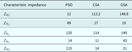
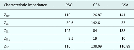
The optimized characteristic impedances of the proposed SOMIs using optimization algorithms are summarized in Tables 2 and 8, respectively.

Table 2.

Optimized characteristic impedances of proposed-1 SOMI

Simulation results

In this section, simulation results are discussed and analyzed. All the simulation results are carried out in MATLAB environment. For the fair comparison of optimization algorithms, same control parameters are selected for PSO, CSA, and GSA. For practical realizability lower and upper bound of the optimized coefficients are set to be at 10Ω and 150Ω. To evaluate the performance of the proposed SOMIs magnitude response, absolute magnitude error (AME), phase response, pole-zero plot, convergence rate and improvement rate are taken into consideration.

Approach-1 [proposed-1 SOMI]

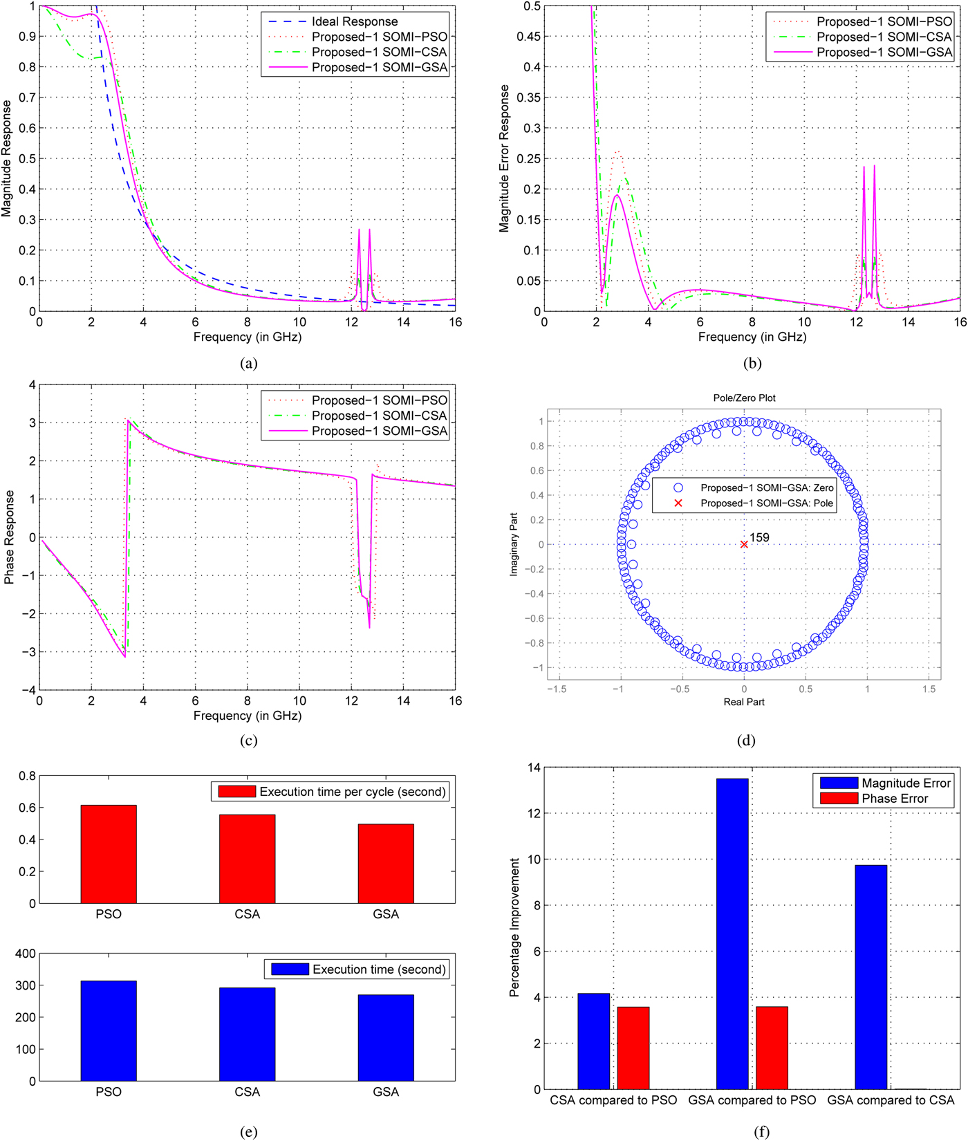
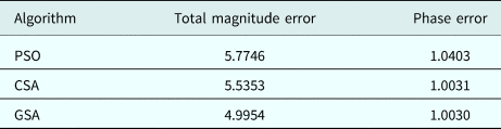
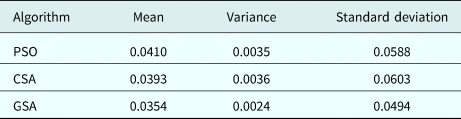
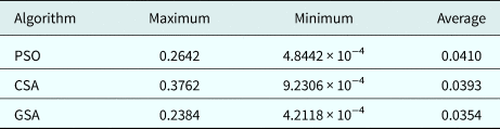
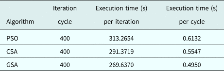
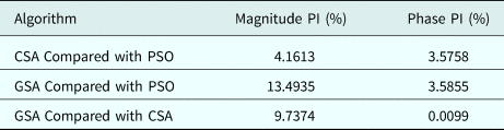
The configuration of the proposed-1 SOMI is shown in Fig. 1 and the optimized characteristic impedances of the proposed-1 SOMI, obtained by PSO, CSA, and GSA are given in Table 2. For the frequency response analysis of the proposed SOMI the magnitude response, AME, phase response, pole-zero plot, fitness rate and improvement graph are the parameters selected as demonstrated in Figs 2(a)–2(f). The total magnitude error = 4.99 phase error = 1.0030 which is reported in Table 3. Table 4 summarizes the statistical analysis of different characteristics such as mean, variance, and standard deviation of magnitude error of the proposed-1 SOMI. It is observed that GSA-based results has least values in all aspects, which are mean error = 0.0354, variance = 0.0024, and standard deviation = 0.0494. The qualitatively analyzed data of magnitude error for the proposed-1 SOMI is reported in Table 5. The maximum error = 0.2384, minimum error = 4.21 × 10⁻⁴, and average error = 0.0354. It is observed that the errors obtained are least values in the case of GSA as compared with the PSO and CSA. Fig. 4(d) shows the pole-zero plot of the proposed-1 SOMI for stability analysis in which all the poles and zeros lies within the unit circle. This plot affirms that the proposed-1 SOMI is stable. Fig. 4(e) shows the convergence profile of all the three algorithms in which it clearly demonstrates that GSA is faster than PSO and CSA in less execution time which is summarized in Table 6 as well. Fig. 4(f) shows the percentage improvement comparison in magnitude error for the proposed-1 SOMI as CSA to PSO, GSA to PSO, and GSA to CSA that is 4.1613, 13.4935, and 9.7374%, respectively, and the percentage improvement comparison in phase errors are 3.5758, 3.5855, and 0.0099%, respectively, which is summarized in Table 7. The magnitude response of the proposed-1 SOMI GSA-based matches closely with that of the ideal one in the frequency range 2.5–16 GHz. Based on the observation, GSA has least magnitude error and highest convergence speed as compared with the PSO and CSA.

Fig. 2.

Profile of proposed-1 SOMI (a) Magnitude response, (b) Magnitude error response, (c) Phase response, (d) Pole-zero plot, (e) Convergence profile, and (f) Improvement bar-graph.

Table 3.

Comparison summary of total magnitude and phase error for proposed-1 SOMI

Table 4.

Statistical data of magnitude error for proposed-1 SOMI

Table 5.

Qualitatively data of magnitude error for proposed-1 SOMI

Table 6.

Convergence profile for proposed-1 SOMI

Table 7.

Percentage improvement in magnitude and phase error forproposed-1 SOMI

Approach-2 [proposed-2 SOMI]

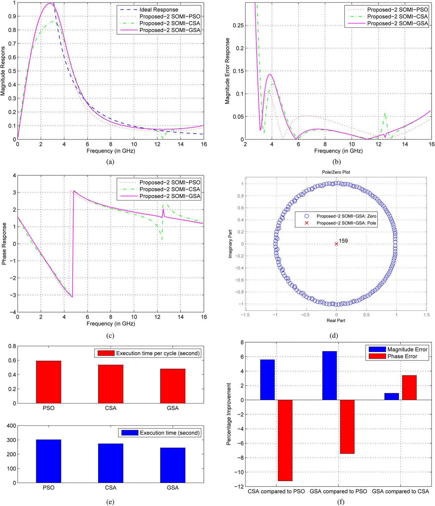
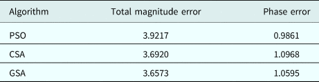
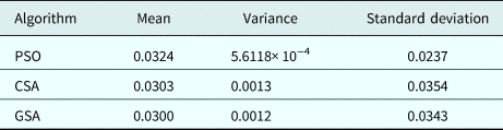
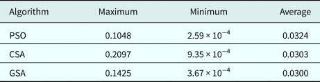
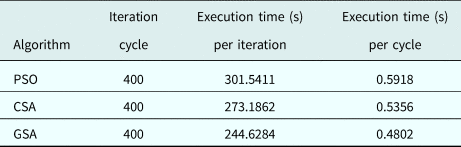
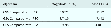
The configuration of the proposed-2 SOMI is shown in Fig. 3 and the optimized characteristic impedances of the proposed-2 SOMI, obtained by PSO, CSA, and GSA are given in Table 8. The same parameters are selected for the frequency response analysis of the proposed-2 SOMI as proposed-1 SOMI which are demonstrated in Figs 4(a)–4(f). The total magnitude error = 3.6573 phase error = 1.0595 which is reported in Table 9. Table 10 summarizes the statistical analysis of different characteristics such as mean, variance, and standard deviation of magnitude error of the proposed-2 SOMI. It is observed that GSA-based results has the least values in all aspects, which are mean error = 0.0.0300, variance = 0.0012, and standard deviation = 0.0343. The qualitatively analyzed data of magnitude error for the proposed-2 SOMI is reported in Table 11. The maximum error = 0.1425, minimum error = 3.627 × 10⁻⁴, and average error = 0.0300. It is observed that the errors obtained are least values in the case of GSA as compared with the PSO and CSA. Fig. 6(d) shows the pole-zero plot of the proposed-2 SOMI for stability analysis in which all the poles and zeros lies within the unit circle. This plot affirms that the proposed-2 SOMI is stable. Fig. 6(e) shows the convergence profile of all the three algorithms in which it clearly demonstrates that GSA is faster than PSO and CSA with less execution time which is summarized in Table 12 as well. Fig. 6(f) shows the percentage improvement comparison in magnitude error for the proposed-2 SOMI as CSA to PSO, GSA to PSO, and GSA to CSA that is 5.8571, 6.7419, and 0.9398%, respectively, and the percentage improvement comparison in phase error are − 11.22, − 7.443, and 3.400%, respectively, which is summarized in Table 13. The magnitude response of the proposed-2 SOMI GSA-based matches closely with that of the ideal one in frequency range 3.0–15 GHz. Based on the observation, GSA has the least magnitude error and highest convergence speed as compared with PSO and CSA.

Fig. 3.

Configuration of the proposed-2 SOMI.

Fig. 4.

Profile of the proposed-2 SOMI (a) Magnitude response, (b) Magnitude error response, (c) Phase response, (d) Pole-zero plot, (e) Convergence profile, and (f) 3Improvement bar-graph.

Table 8.

Optimized characteristic impedances of proposed-2 SOMI

Table 9.

Comparison summary of total magnitude and phase error for proposed-2 SOMI

Table 10.

Statistical data of magnitude error for proposed-2 SOMI

Table 11.

Qualitatively data of magnitude error for proposed-2 SOMI

Table 12.

Convergence profile for proposed-2 SOMI

Table 13.

Percentage improvement in magnitude and phase error forproposed-2 SOMI

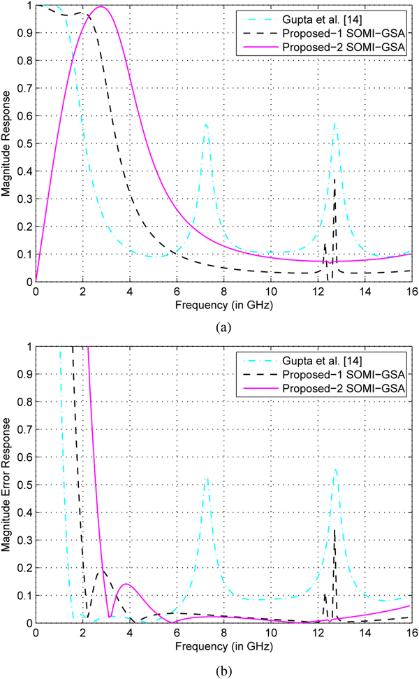
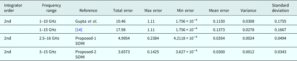
Figure 5 depicts the comparison of the proposed SOMIs with the existing second order microwave integrator. The comparative magnitude response and AME of the proposed SOMI GSA-based optimization with existing integrator are shown in Figs 5(a) and 5(b), respectively. Table 15 demonstrates the corresponding qualitatively and statistical analysis of magnitude error of the proposed SOMIs and existing integrator. Fig. 5 and Table 15 confirms that the proposed SOMIs GSA-based are more appropriate in terms of magnitude, least magnitude error, and wide band-width, specifically for high-frequency range.

Fig. 5.

Comparison of the proposed SOMI-GSA with existing integrator. (a) Magnitude response and (b) Error response.

Table 14.

Comparison of magnitude error of the proposed SOMIs with existing design method

Table 15.

Detailed dimensions

The results of the proposed-2 SOMI GSA-based leads in performance to the proposed-1 SOMI counterpart. All simulation results of the proposed-2 SOMI approximates with the ideal one and have linear phase response in its frequency range 3.0–15 GHz. Therefore the proposed-2 SOMI is implemented by using microstrip lines.

Implementation of wideband SOMI

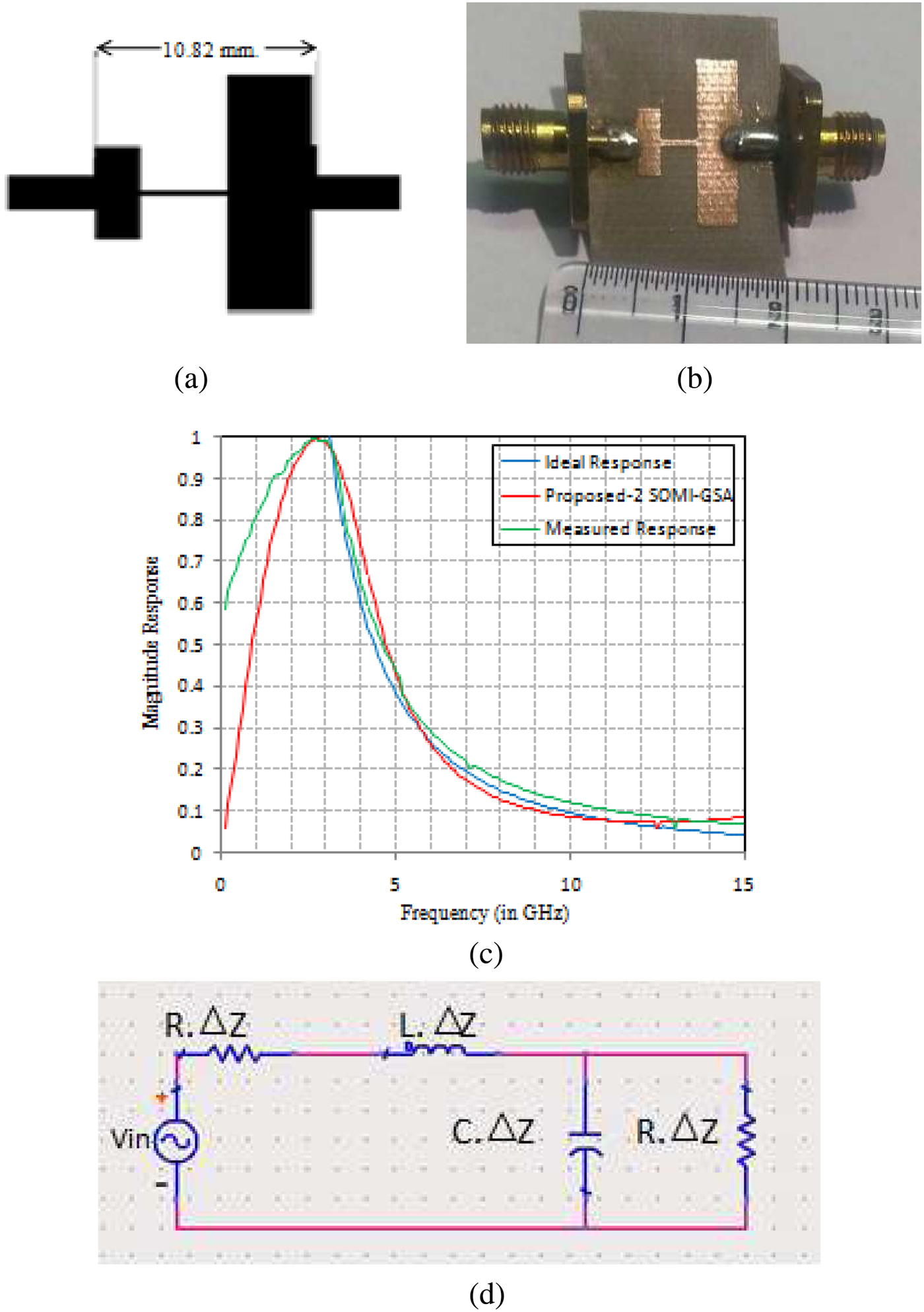
Microstrip lines are used to implement SOMI, which have l = λ₀/4, where l represents the physical length of line elements(stubs and transmission lines) and λ₀ represents the wavelength at the normalized frequency, that is 12.5 GHz. The physical length of each section (stubs and transmission lines) is set to be 90° at the normalizing frequency. To implement proposed-2 SOMI, RT/Duroid substrate is used having dielectric constant ε_r = 2.2, height of substrate (H) = 30 mil (0.762 mm), loss tangent (tanδ) = 0.001, and copper cladding is 35 um. The values of characteristic impedances for proposed-2 SOMI GSA-based from left to right are 141.23, 33.24, 138.23, 10, 116.89 Ω, and Z ₀ is reference impedance, that is 50 Ω. The layout and fabrication of proposed-2 wideband SOMI are shown in Figs 6(a) and 6(b), respectively. The total length of the proposed-2 SOMI is 10.82 mm or 426 mil excluding the reference line from both sides as shown in Fig. 6(a). The detailed dimension of proposed-2 SOMI is reported in Table 15. The transmitted parameter S ₂₁ is measured by using an Agilent VNA.

Fig. 6.

Profile (a) Layout with dimension, (b) Physical layout of the proposed-2 SOMI (c) Measured magnitude response (d) Lumped equivalent model.

The measured magnitude response of S ₂₁ of the proposed-2 SOMI GSA-based with its ideal and simulated magnitude response is demonstrated in Fig. 6(c). It is distinct from Fig. 6(c) that the measured magnitude response is consistent with its ideal response in the frequency range 3–15 GHz. The lumped element equivalent circuit of the proposed-2 SOMI is shown in Fig. 6(d). Consider infinitesimal length of transmission line for lumped element equivalent circuit where R, L, C are per unit length quantities. In broadband applications, lumped elements play a significant role in achieving the required circuit performance. Lumped elements have smaller size, lower cost, large impedance transformation ratio capability, smaller interaction effects between circuit elements, lower associated complementary reactance, and wider bandwidth capability. Lumped element equivalent circuit modeling using lumped inductors with lower parasitic capacitance will result in wider bandwidth circuit [Reference Bahl30].