I. INTRODUCTION
Owing to the unique and excellent properties of carbon nanotubes (CNTs), CNTs embedded in polymer composite have captured much attention in the field of novel conductive and multifunctional material.Reference Yoon and Jang1,Reference Georgousis, Pandis, Kalamiotis, Georgiopoulos, Kyritsis, Kontou, Pissis, Micusik, Czanikova and Kulicek2 There are many potential applications of these nanocomposites. In particular, it is being investigated as stretchable and flexible piezoresistive material through combining CNTs with highly elastic polymer for advanced application, including electronic skin, wearable devices, health monitoring, and so forth.Reference Ryu, Lee, Chou, Xu, Zhao, Hart and Kim3,Reference Pang, Koo, Nguyen, Caves, Kim, Chortos, Kim, Wang, Tok and Bao4
Comparing to other conductive materials, CNTs have significant advantages, such as large aspect ratio (AR), superior electrical conductivity, and excellent compatibility with polymer matrices.Reference Nan, Shen and Ma5 Due to their curvilinear tube shape, it is apt to build a three-dimensional (3D) network in the polymer, which is helpful for the CNTs/polymer composite to be a kind of sensitive piezoresistive material. Also, owing to the diversity of CNTs, CNTs/polymer composites present a variety of piezoresistivity characteristics. Their gauge factor (GF) ranges from 0.74 to 50 with different types of CNTs.Reference Hu, Fukunaga, Atobe, Liu and Li6 To find the factors that influence piezoresistivity of these composites based on CNTs/polymer, simulation and modeling is a crucial and practical approach.
Although recently many numerical and theoretical studies aimed at understanding the principle of electrical characteristics, there are few studies comprehensively investigating the piezoresistivity at and after percolation threshold through a realistic composite model.Reference Panozzo, Zappalorto and Quaresimin7,Reference Taherian8 Moreover, to determine percolation threshold, the empirical percolation method and power law are currently the typical ways to analyze the electrical conductivity and piezoresistivity.Reference Theodosiou and Saravanos9,Reference Xu, Rezvanian, Peters and Zikry10 To some extent, it is not sufficient to exhibit a clear view of the electrical conductivity variation along with the increasing of the conductive filler concentration. In particular, the critical percolation threshold is not a definite value, but a range of values. Furthermore, in the range of values, the electrical conductivity varies quite significantly. This problem was neglected by pioneering work. Hence, the range of percolation threshold should be further investigated.
Amini et al. merely proposed the concentration close to the percolation threshold that would give the composite a higher sensitivity but did not specify whether the value should be more than the percolation threshold or not.Reference Amini and Bahreyni11 Hu et al. have developed a 3D CNTs/polymer model to analyze its electrical behavior, while they did not further investigate piezoresistivity.Reference Hu, Masuda, Yan, Yamamoto, Fukunaga and Hashida12 They only pointed out the sensitivity which primarily depends on the tunneling resistance and the ratio of the tunneling resistance to total resistance.Reference Hu, Karube, Arai, Watanabe, Yan, Li, Liu and Fukunaga13,Reference Hu, Karube, Yan, Masuda and Fukunaga14 For the highly stretchable polymer, the properties of the polymer play an essential role in deciding on the piezoresistivity.Reference Wang and Ye15–Reference Wang, Weng, Meguid and Weng17 Wang and Ye defined a value called the average junction gap variation to describe the piezoresistivity and obtained an optimizing principle for CNTs/polymer composites.Reference Wang and Ye15 Nevertheless, the principle still needs to be verified because they obtained it through a static model, not through a dynamic model. Therefore, a comprehensive theoretical study through a dynamic model to systemically find the key parameters influencing piezoresistivity is necessary.
This paper makes an elaborate study on the mechanism and principle of CNTs/polymer composites through building a randomly dynamic 3D model. At first, after calculation of a set of numerical simulations, the critical percolation threshold range (PTR) for piezoresistivity behavior is found and defined. Subsequently, parameters influencing the piezoresistivity were considered, for example, AR, the electrical conductivity of CNTs and concentration, alignment of CNTs, and Poisson’s ratio (PR) of the polymer.
II. MODELING AND SIMULATION
A. Building the model
To investigate the electrical properties of the CNTs/polymer composite theoretically, a 3D representative composite model is required to be randomly generated and basic assumptions are defined as follows:
(i) Due to the insulation of polymers, the composite can be regarded as an equivalent conductive resistor network connected by CNTs.
(ii) In the model, a single CNT is treated as a soft-core cylinder and can be penetrated or overlapped by other CNTs.
(iii) It is assumed that the CNT is straight for accelerating computation and also its AR not very large (from 50 to 200). Despite the curvilinearity of CNTs, the factors influencing the electrical properties would not be changed.
The CNT is defined by the length L, diameter D, and electrical conductivity of CNTs σCNT, with the AR being AR = L/D, as shown in Fig. 1(a). The length and diameter can be randomly generated subject to Gaussian distribution. As the model has a limited boundary, some CNTs penetrating through the boundary surface should be cut down. Noticeably, the AR is an approximate value, but it has little influence on the precision of simulation.
(a) Parameters of a 3D CNT, (b) definition of location and orientation of a CNT and (c) the schematic of an electrical conductive CNT network and tunneling effect in the resistor network.

To randomly generate CNTs, the position of a CNT is created by generating a midpoint P(x, y, z), while the orientation of a CNT can be defined using azimuthal angle φ and polar angle θ, as depicted in Fig. 1(b). These parameters of CNTs could be calculated usingReference Wang and Ye15
 $$x = {l_x} \times {\rm{rand}}\quad ,$$
 $$y = {l_y} \times {\rm{rand}}\quad ,$$
 $$z = {l_z} \times {\rm{rand}}\quad ,$$
 $$\theta = \pi \times {{\left( {1 - 2 \times {\rm{rand}}} \right)} \over {2 \times {\rm{ori}}}}\quad ,$$
 $$\varphi = 2\pi \times {\rm{rand}}\quad ,$$
where l x, l y, and l z are the side lengths of the model, and rand is a randomly generated value ranging from 0 to 1. In fact, the model is set as a cube so that l x, l y, and l z are equal to each other. With the aim to reduce the occasion of the simulation, a dimension coefficient associated with the model is created to describe the relationship between the length of the side and the average value of CNT length L. l m = C v × l a, where the l m is the side length of the cube model, so l x = l y = l z = l m. C v is the dimension coefficient and l a is the mean of the CNT. Notably, l a is set as 1. We managed to set the coefficient ranging from 2 to 4. When the coefficient is 2, the results may be generated with considerable discrepancy. As for the coefficient of 4 or larger, the following calculation like electrical conductivity evaluation and piezoresistivity would spend more time. Hence, we set the coefficient as 3. ori is the coefficient for the maximum polar angle of a CNT. Here, the default setting of ori is 1. Subsequently, the coordinates of two endpoints can be expressed as follows:
 $${x_{\rm{e}}} = x \pm {l \over 2} \times \sin \theta \times \cos \varphi \quad ,$$
 $${y_{\rm{e}}} = y \pm {l \over 2} \times \sin \theta \times \sin \varphi \quad ,$$
 $${z_{\rm{e}}} = z \pm {l \over 2} \times \cos \theta \quad ,$$
where x e, y e, and z e are the coordinates of two endpoints and l is the length of the CNT. According to this, thousands of CNTs can be generated randomly in the cube model.
B. Resistance calculation
To obtain the total resistance of the cube model, different types of resistance should be sorted out and calculated. There are two kinds of resistance, the contact resistance between CNTs and the inherent CNT resistance, as depicted in Fig. 1(c). Actually, CNTs hardly touch each other in practice due to the existence of van der Waals force, instead, contacting CNTs would happen to be deformed.Reference Gong, Zhu and Meguid18,Reference Ambrosetti, Grimaldi, Balberg, Maeder, Danani and Ryser19 Imperfect interface condition between adjacent CNTs and polymer matrix leads to increasing electrical resistance.Reference Wang, Weng, Meguid and Weng17 Also, the interface conductivity can be enhanced by electrical tunneling effect so that the interfacial resistance should be evaluated theoretically through combining contact resistance with tunneling resistance.Reference Wang, Weng, Meguid and Weng17,Reference Wang, Weng, Meguid and Hamouda20 However, Alborz et al.Reference Amini and Bahreyni11 and Hu et al.Reference Hu, Masuda, Yan, Yamamoto, Fukunaga and Hashida12 insisted on assuming that the CNTs could be assumed to penetrate with each other with perfect interface. Hence, the interfacial resistance was only considered as the tunneling resistance without consideration of contacting resistance in their simulations. In light of the computational cost, this work assumes that CNTs could perfectly penetrate with each other without contact resistance. Therefore, in the cube model, if the distance d, between the centerlines of CNTs, is smaller than the diameter of CNT, the contact resistance can be neglected, whereas the contact resistance is regarded as tunneling resistance, when d is larger than D and shorter than the critical tunneling distance. The tunneling resistance R T as the primary contact resistance is calculated byReference Simmons21
 $${R_{\rm{T}}} = {V \over {AJ}} = {{{P^2}h} \over {A{e^2}\sqrt {2m\lambda } }}\exp \left( {{{4\pi h} \over h}\sqrt {2m\lambda } } \right)\quad ,$$
where J is the tunneling current density and V is the electrical potential difference with A being the cross-sectional area of the tunnel. P is Planck’s constant, e and m are the charge quantum and mass of an electron, respectively. h is the minimal distance between the surfaces of two adjacent CNTs. It can be obtained by d–D. It needs to be noted that the cut-off distance for the tunneling effect is set to be 1.8 nm according to previous work.Reference Li, Thostenson and Chou22 λ is the barrier height of the polymer matrix (around 0.5–2.5 eV) and 1.5 eV was selected here.Reference Hu, Karube, Yan, Masuda and Fukunaga14
The different network structures of CNTs induce different inherent resistances. As shown in Fig. 1(c), the active conductive segments are merely the connected paths, which also connect the end electrodes of the cube model. Besides the conductive section of a CNT, L ij is the length between contacting junctions i and j as depicted in Fig. 1(c). Therefore, the resistance and the electrical conductivity of the active conductive segment of a CNT can be calculated by
 $${R_{ij}} = {{4{L_{ij}}} \over {{\sigma _{{\rm{CNT}}}}\pi {D^2}}},\quad {C_{ij}} = {1 \over {{R_{ij}}}}\quad ,$$
where L ij is the distance between two contacting points i and j. R ij and C ij are the resistance and conductivity of the effective conductive segment of a CNT, respectively.
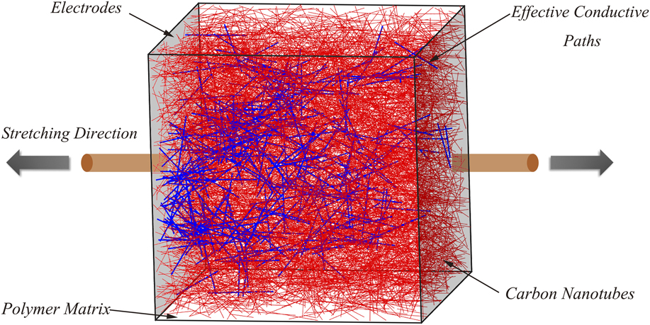
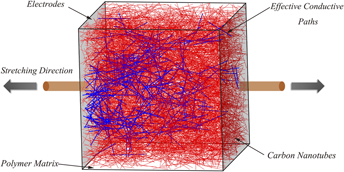
The next step is to find the active conductive network in the cube model along the voltage direction. In this work, all the contacting junctions are first marked and then clusters which do not connect to the end surfaces applied on voltages should be deleted. Notably, to accelerate the computation, the cube model is divided into small regions so that only CNTs in the same region need to verify whether it is in contact. After that, some redundant paths of CNTs should be removed.Reference Amini and Bahreyni11 As indicated in Fig. 2, the bold blue lines are percolating CNTs and thin red lines are CNTs without electrical current. Based on the concise resistor network under an applied voltage and Kirchhoff’s current law, the total electrical current at every node can be written as follows:
 $${I_i} = \sum\limits_j^{{N_i}} {{C_{ij}}\left( {{V_i} - {V_j}} \right)} \quad ,$$
where N i is the total number of nodes near the node i, and V i and V j are the electrical potentials of points i and j. The potential of nodes situated on the positive and negative electrodes are assumed to be 200 and 0, respectively. Hence, the linear sparse matrix is listed and estimated using the Biconjugate gradients (BICG) method.Reference Barrett, Berry, Chan, Demmel, Donato, Dongarra, Eijkhout, Pozo, Romine and Van der Vorst23 After the total electrical current I is acquired, the macroscopic electrical resistance R m of the model can be estimated by Ohm’s law. Then its electrical conductivity can be calculated based on the formula 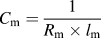 ${C_{\rm{m}}} = {1 \over {{R_{\rm{m}}} \times {l_{\rm{m}}}}}$, where C m is the electrical conductivity of the model.
A 3D representative cube model with conductive paths depicted using blue bold lines.

C. Piezoresistivity simulation
As for the piezoresistivity, it is assumed that the polymer is highly stretchable, so the positions and orientations of CNTs would have an apparent change. Here, the widely accepted re-orientation model simulation is adopted to study the response of CNTs under applied strain.Reference Hu, Fukunaga, Atobe, Liu and Li6,Reference Amini and Bahreyni11,Reference Wang and Ye15,Reference Gbaguidi, Namilae and Kim24,Reference Taya, Kim and Ono25 This model simplifies the strain variation without consideration of the local strain around CNTs. That is to say, the movement of CNTs would not be influenced by the polymer matrix. The Young’s modulus of the CNT is far bigger than the polymer matrix so that the polymer’s body is considered to absorb all of the applied stress and strain in nanotubes is neglected.Reference Amini and Bahreyni11 Even though there are other complicated models built to simulate the strain variation regarding the CNTs/polymer composite, they mainly concentrated on the mechanical properties instead of electrical properties.Reference Shokrieh and Rafiee26–Reference Mohammadpour, Awang, Kakooei and Akil28 For instance, Shokrieh et al.Reference Shokrieh and Rafiee26 used Newton–Raphson iterative method to analyze the nonlinear behavior of the van der Waals force to simulate the CNT movement when the model was stretched. Mohammadpour et al.Reference Mohammadpour, Awang, Kakooei and Akil28 also built a nonlinear representative volume element of the composite to predict its mechanical behavior. In this model, CNTs are thought as nondeformable and their deformation is neglected since the Young’s modulus of the polymer (i.e., PDMS is only 1 MPa at most) is much smaller than that of CNTs (around 1 GPa). As a consequence, the new position and orientation of a CNT can be expressed as Eq. (6) after stretched in a uniaxial direction of X-axis seen in Fig. 2.Reference Wang and Ye15
 $$\left\{ {\matrix{ {x'} \cr {y'} \cr {z'} \cr} } \right\} = \left[ {\matrix{ {1 - \upsilon \times \varepsilon } & 0 & 0 \cr 0 & {1 - \upsilon \times \varepsilon } & 0 \cr 0 & 0 & {1 + \varepsilon } \cr} } \right]\left\{ {\matrix{ x \cr y \cr z \cr} } \right\}\quad ,$$
 $$\theta ' = {\tan ^{ - 1}}\left( {{{1 - \varepsilon \times \upsilon } \over {1 + \varepsilon }} \times \tan \theta } \right)\quad ,$$
 $$\varphi ' = \left\{ {\matrix{ {{{\tan }^{ - 1}}\left( {{{1 - \varepsilon \times \upsilon } \over {1 + \varepsilon }}\tan \varphi } \right),} \hfill & {0 \lt \varphi \lt {\pi \over 2}} \hfill \cr {{{\tan }^{ - 1}}\left( {{{1 - \varepsilon \times \upsilon } \over {1 + \varepsilon }}\tan \varphi } \right) + \pi ,} \hfill & {{\pi \over 2} \lt \varphi \lt {{3\pi } \over 2}} \hfill \cr {{{\tan }^{ - 1}}\left( {{{1 - \varepsilon \times \upsilon } \over {1 + \varepsilon }}\tan \varphi } \right) + {{3\pi } \over 3},} \hfill & {{{3\pi } \over 2} \lt \varphi \lt 2\pi } \hfill \cr} } \right.\quad ,$$
where x′, y′, and z′ are the new coordinates of the midpoint of a CNT after a strain (ε) is applied, while θ′ and φ′ are the updated angle. υ stands for the PR of the composite. The coordinates of two end points can be calculated based on Eq. (2).
The stretched cube model of the composite is then updated, so the new network of the resistor is formed as well. Repeating the above-mentioned procedure, the electrical resistance and conductivity will be re-evaluated. For better observing the piezoresistivity, the GF is introduced which is defined as follows:
 $$GF = {{\Delta R/R} \over \varepsilon }\quad ,$$
where R is the initial resistance and ΔR is the difference between the value of resistance after being stretched and the initial value.
III. RESULTS AND DISCUSSION
To better determine the dominant factors that influence the static electrical properties and piezoresistivity of the composite, it is assumed that CNTs dispersed evenly in the polymer without agglomeration. Several common factors are taken into consideration here, including CNT concentration, AR of CNTs, and the electrical conductivity of CNTs, PR of the composite as well as the direction of CNTs.
A. Static electrical behavior analysis
Previously, researchers regarded the percolation threshold as the best concentration to make sensors considering that sensors were only capable of experiencing small strain.Reference Ferreira, Martínez, Ansón-Casaos, Gómez-Pineda, Vaz and Lanceros-Mendez29 However, this is not suitable for the current highly stretchable sensor. This is attributed to the fact that it has no conductivity after drastically stretching due to damage to the CNTs’ network.
1. Influence of CNT volume fraction
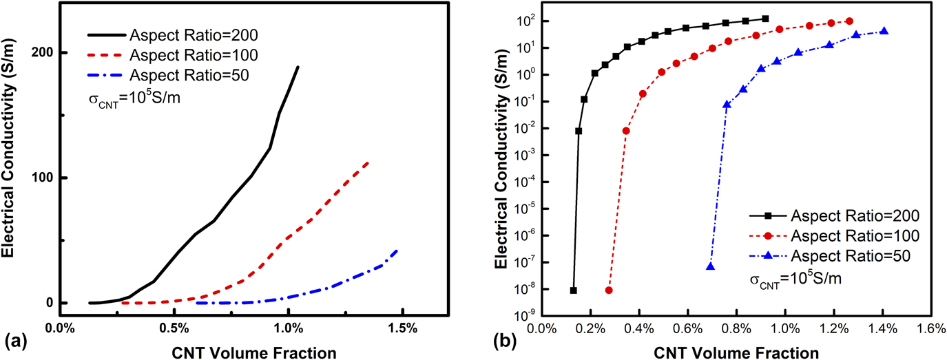
After 100 times simulation, the maximum likelihood estimator (MLE) of the electrical conductivity of the model was obtained through Poisson distribution, and the correlation between MLE of electrical conductivity and CNT volume fraction (CVF) was plotted. As shown in Fig. 3(a), all the electrical conductivities for CNTs with different ARs experience an exponential rise. If the AR of CNTs becomes larger, the slope of the curve of conductivity against CVF will be enlarged. Meanwhile, the starting percolation threshold would be rather different. Along with AR decreasing, the larger CVF is needed to construct the conductive network in the cube model. It can be clearly seen in Fig. 3(b) that the starting percolation threshold for AR 200 is just around 0.18% of CVF, whereas it is required to be 0.3% and 0.7% for AR 100 and 50, respectively, assuming that 10−6 S/m is the threshold value to be conductive. After threshold, the conductivity should vary following the power law
 $$\sigma = {\sigma _0}{\left( {p - {p_{\rm{c}}}} \right)^t}\quad ,$$
where σ, σ0, and p are the electrical conductivity of composite, the intrinsic conductivity of CNTs, and the volume fraction of CNTs, respectively. p c is the percolation threshold and t is the critical exponent. The variation process of electrical conductivity in Fig. 3(b) exhibits agreement with this formula.
The relationship between CVF and electrical conductivity of the composite with different ARs using linear scale (a) and logarithmic scale (b).

To further validate the model, the Bruggeman effective medium theory for electrical conductivity of the electronic composite is used for contrast.Reference Gao, Zhou and Ding30–Reference Gao and Li32 Based on this theory, an equation is given as follows:
 $$9\left( {1 - f} \right){{{K_{\rm{m}}} - K} \over {2{K_{\rm{m}}} + K}} + f\left[ {{{{K_{\rm{c}}} - K} \over {K + {L_x}\left( {{K_{\rm{c}}} - K} \right)}}} \right] = 0\quad ,$$
where f denotes the CVF while K is the electrical conductivity of the composite. K c and K m are the electrical conductivities of the CNTs and the polymer matrix, respectively. Here, K c is set as 105 S/m and K m is assigned with 10−13 S/m. L x is the depolarization factor depending on the AR of CNTs which can be expressed as
 $${L_x} = {1 \over {2{{\left( {{\rm{A}}{{\rm{R}}^2} - 1} \right)}^{3/2}}}}\left[ {{\rm{AR}}\ln {{{\rm{AR}} + \sqrt {{\rm{A}}{{\rm{R}}^2} - 1} } \over {{\rm{AR}} - \sqrt {{\rm{A}}{{\rm{R}}^2} - 1} }} - 2\sqrt {{{A}}{{{R}}^2} - 1} } \right]\quad .$$
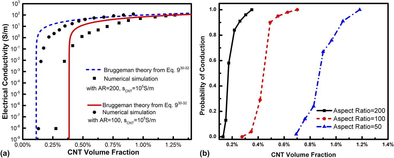
L x is equal to 0.0004299 and 0.0001248 for AR 100 and 200, respectively. The projection generated by our model is then compared with the Bruggeman theoretical estimation from Eq. (9) as depicted in Fig. 4(a). With regards to both CNTs with AR 100 and 200, the projection produced by this paper shows a moderate agreement with the Bruggeman theoretical estimation.
(a) The comparison between the Bruggeman theoretical estimationReference Gao, Zhou and Ding30–Reference Gao and Li32 and the evaluation of electrical conductivity of the composite in this paper and (b) the relationship between the probability of conduction and the CVF for composites models with different ARs.

In the 100 simulations, some results show no electrical conductivity around percolation threshold. Notably, the criterion to judge whether the composite model is electrically conductive or not is set as the electrical conductivity of 10−6 S/m. As is well-known, the electrical conductivity of 10−8 S/m is the threshold for material transition from insulator to semiconductor. Therefore, we amplified two magnitudes of this value to guarantee that these results can be definitely envisioned as semiconductor or conductor. On the one hand, this is attributed to the fact that the model is not large enough. On the other hand, due to the network is randomly formed, it cannot be guaranteed that the conductive paths appear every time. Hence, the probability of conductivity was taken into account along with the variation of CVF. The likelihood of conductivity means that the probability to produce the conductive paths of CNTs in the composite model. As depicted in Fig. 4(b), it can be seen that when the CVF for AR 200 reaches around 0.3%, the probability of conduction is 100%, whereas the CVF for AR 100 and 50 are 0.6% and 1.2%, respectively. It means that the composite model must be conductive after this value, provided that CNTs are dispersed evenly and randomly. Thus it can be called the ending percolation. The CVF between these two values is defined as PTR in this work. Notably, the PTR is wider for AR 50 than the other two. It can be explained that CNTs are difficult to touch with other CNTs at the same CVF when the AR is lower. Thus, even if CVF was considerably large, the model still probably shows no conductivity. As a result, if the AR of CNTs is larger, lower CVF is needed and the probability of conductivity is improved. Nevertheless, it is much more difficult to disperse CNTs without agglomeration using CNTs with large AR, due to the effect of van der Waals force.
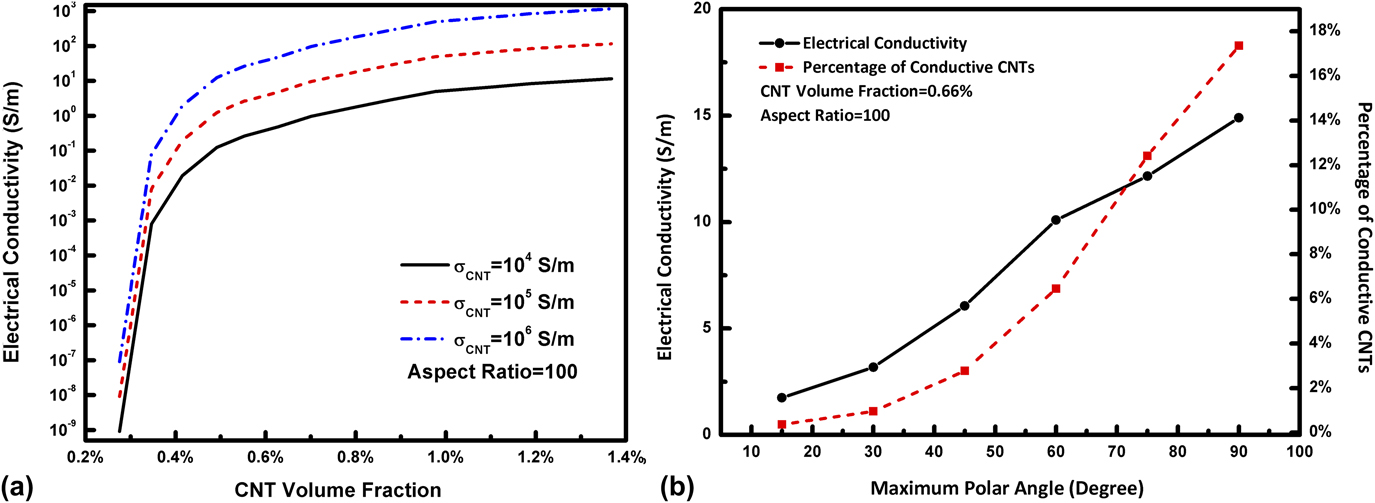
Except for the CVF, the intrinsic electrical conductivity of CNTs and the orientation of CNTs would influence the electrical conductivity of the composite as well. It can be seen in Fig. 5(a) that the electrical conductivity of the composite can be enhanced as the electrical conductivity of CNTs grows. However, the variation process does not change because the connected paths have no change in the model. As to the orientation of CNTs, only the polar angle was taken into consideration, which is controlled by the parameter Ori mentioned above. The azimuthal angle has little effect on the electrical conductivity along the z-axis direction so that it is generated ranging from 0 to 2π.
(a) Influence of the electrical conductivity of CNTs on the electrical conductivity of composites and (b) the relationships between the maximum polar angle and the electrical conductivity of the composite as well as the percentage of connected CNTs.

2. Influence of CNT polar angles
To investigate the relationship between the polar angle and electrical conductivity, the maximum polar angle is introduced. Along with the growth of maximum polar angle, the electrical conductivity turns better, as indicated in Fig. 5(b). When the maximum angle is 15°, that is to say, CNTs are nearly parallel with each other, it is difficult to have junctions so that connected paths would hardly be formed. The number of conductive CNTs will also increase as the maximum polar angle become larger [red dashed line in Fig. 5(b)]. It means that the electrical conductivity would be improved if the extent of alignment of CNTs is worse, which would give more chances of CNTs contacting with each other. It can also explain why the resistance of stretchable composites would go up after stretching to some extent, due to the orientation of CNTs turning consistent.
B. Piezoresistivity analysis
Piezoresistivity is more complicated to analyze, compared with the static electrical behavior. It does not only relate to the properties of CNTs but also involves mechanical properties of the polymer matrix.
1. Effect of CVF on piezoresistivity
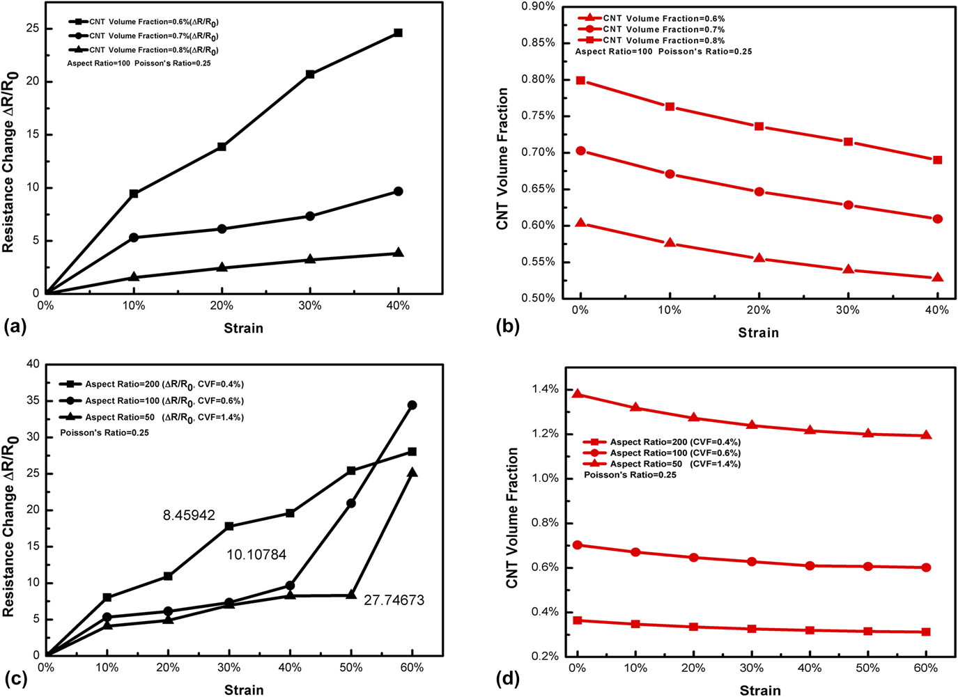
As is well known, CVF plays an important role in influencing the piezoresistivity. Hence, the CVF is first studied through simulation. Assuming that PR of the composite is 0.25 and the AR of CNTs is 100, the relationship between tensile strain and resistance change (the difference between initial resistance and current to initial resistance) can be described as shown in Fig. 6(a). Three different CVFs (i.e., 0.6, 0.7, and 0.8%) are selected for comparison, which are slightly bigger than ending percolation threshold. It is worth mentioning that in spite of the influence of CVF on PR, the PR for the models with different CVFs is similar.Reference Hu, Fukunaga, Lu, Kameyama and Yan33 The resistance of the composite increases while the model is being continuously stretched. It is observed that the GF of the model with CVF 0.6% is the largest among them [the slope of the function between strain and resistance change depicted in Fig. 6(a)] while that of CVF 0.8% is the least. This is because it has the high probability for CNTs to contact with each other with larger CVF. This means that when the material was stretched, more junctions and conductive paths are left behind. In addition, once the cube model is uniformly stretched, due to the influence of the composite PR, the CVF will change. Therefore, when the tensile strain is applied, not only the resistance change will occur but also the CVF will vary as well. The CVF variation under applied tension strain is depicted in Fig. 6(b). It can be clearly seen that all of the models with different CVFs exhibit the downward trend, which indirectly reflects the decreasing probability of mutual contacting of CNTs.
The relationship between strain and resistance change for composites models (a) with different CVFs and (c) with different ARs as well as CVFs. The correlation between CVF variation and strain for composites models (b) with different CVFs and (d) with different ARs as well as CVFs.

2. Effect of AR on piezoresistivity
As for the AR of CNTs, it shows little significance to compare the piezoresistivity for models with similar CVFs and different ARs. Hence, the models whose CVFs are slightly larger than ending percolation threshold are more suitable to be selected for comparison (0.4% for AR 200, 0.6% for AR 100, 1.4% for AR 50). Notably, if the CVF is selected in the PTR, the electrical conductivity would become zero within small strain due to the lack of sufficient conductive paths in the model. Meanwhile, the electrical conductivity is similar for AR 100 and AR 200, whereas the model of AR 50 has 27.74673 S/m. As shown in Fig. 6(c), which described the relative change in resistance as a function of strain variation, it can be seen that the GF for AR 200 is the largest before the strain is 0.4. After strain goes over 0.4, the GF for AR 100 suddenly increases, overpassing that of AR 200, while the GF for AR 50 also surges after strain 0.5. This can be explained by the fact that the conductive paths have a significant decline in the model at that time, resulting in the considerable rise of the resistance. In parallel, with the rise of strain, the CVF also experiences decline as displayed in Fig. 6(d). Interestingly, the downward trend is slower for the model composed of CNTs with smaller AR. For the highly stretchable sensor, stretchability and stability are as essential as sensitivity. Obviously, CNTs with large AR are the better choice to be the candidate material for the stretchable sensor. Although intrinsic electrical conductivity of CNTs influences the electrical conductivity of the composite, the conductive paths in the composite have no relationship with it. Naturally, the inherent electrical conductivity of CNTs has little influence on the piezoresistivity.
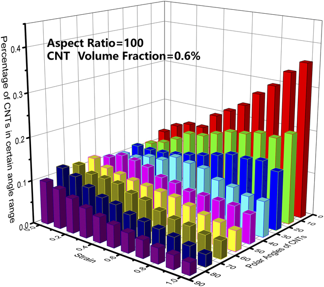
The reason why the electrical conductivity of the composite decreases when it is stretched is attributed to the CNTs aligning gradually during the stretching process. As depicted in Fig. 7, at the initial phase, CNTs have different polar angles distributing evenly from 0° to 90°. However, when it is stretched continuously, the number of CNTs with small polar angles increases gradually, on the contrary, the quantity of CNTs with large polar angles has an apparent decline. It means that the orientation of CNTs becomes parallel to the stretching direction. As mentioned in Sec. III.A, if the extent of alignment of CNTs along the stretching direction is higher, the electrical conductivity will go down. This is why the resistivity of the composite will grow when it suffers intense stretch.
Variation of the distribution state of polar angles of CNTs along with strain increasing.

3. Effect of PR of the matrix on piezoresistivity
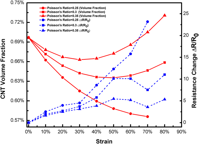
The property of CNTs plays a vital role in determining the piezoresistivity, though the mechanical properties of the polymer matrix also have a significant influence on it. CNTs have a bigger Young’s modulus than that of high stretchable polymers (like PDMS), so the Young’s modulus of polymers plays a negligible part in the piezoresistivity of the composite. Nevertheless, with regard to PR, the different deformation on the transverse surface under axial stretching would result in different resistance variations. Here, we compared CNTs with different PRs (0.25, 0.3, and 0.35) and the same CVF. The CVF variation and the resistance change were plotted along with the increase of tensile strain. It can be found that in Fig. 8 that the resistance of CNTs with PR 0.25 keeps going up, while the other two happen to fluctuate after 50% strain. It can be explained that their CVFs do not go down but rise after 50%, so it gives more opportunities for CNTs to contact each other. On the contrary, CVF for PR 0.25 maintains going down until there are no conductive paths found. Notably, the resistance for PR 0.3 and 0.5 grow again. This is attributed to the alignment of CNTs in spite of the increase of CVF. Besides, the GF will rise when the PR is smaller. Consequently, if the PR is lower, the piezoresistivity will be enhanced.
Resistance changes and the CVF variation along with strain growing for composites models with different PRs.

IV. CONCLUSION
The mechanism of the electrical behavior of highly stretchable CNTs/polymer composite was analyzed through this dynamic 3D model. It is shown that the electrical conductivity of the composite is dependent on the structure of the CNT network in the polymer. Meanwhile, the concept of PTR is proposed, instead of the fixed value of percolation threshold in the previous literature. The PTR is primarily determined by the AR of CNTs and orientation of CNTs provided that CNTs dispersed evenly without agglomeration. The electrical conductivity of CNTs cannot affect PTR but determine the electrical conductivity of the composite. For the stretchable sensors, the CVF which is slightly bigger than ending percolation threshold is a better option for fabricating sensors. As for the piezoresistivity, once the CVF is beyond PTR, the GF will reduce as the CVF increase. Also, higher AR of CNTs will not only make GF better but also will be favorable to keep GF stable. PR of the composite plays an important part on influencing piezoresistivity. With lower PR, GF will be better. Furthermore, if PR is large, the GF will fluctuate once the strain is large. To conclude, CNTs with larger AR and CVF slightly higher than PTR, lower PR of the composite are positive to improve the piezoresistivity and stability of the highly stretchable sensor. Nevertheless, to improve the accuracy of the simulation, in future, we will try to build a more complicated and realistic model to analyze piezoresistivity of the stretchable CNTs/polymer composites.