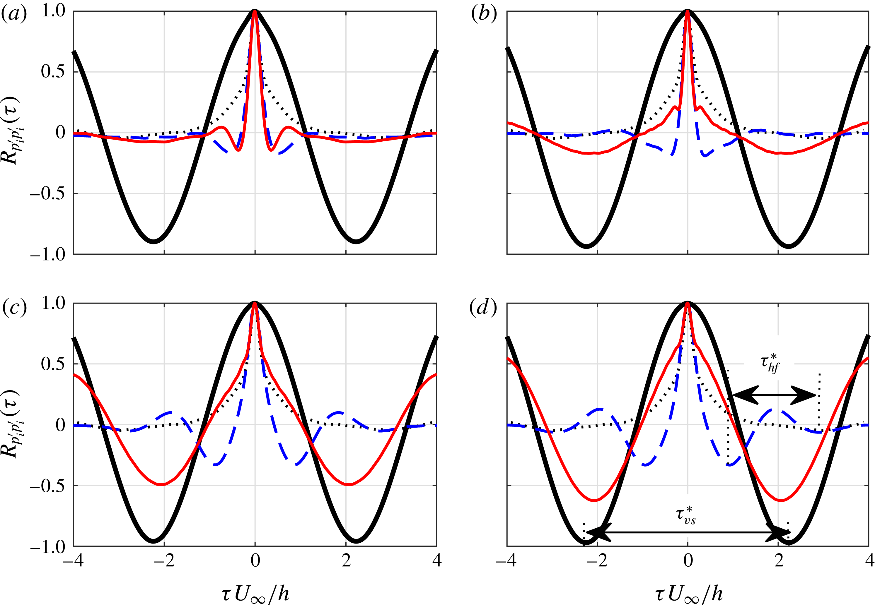
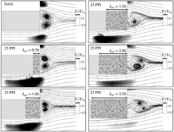
1 Introduction
Turbulent flows and aerodynamically generated noise and vibration are ubiquitous in various engineering applications, in particular for those involving bluff bodies and airfoils. Different passive flow control methods, such as serrations (Lyu, Azarpeyvand & Sinayoko Reference Lyu, Azarpeyvand and Sinayoko2016; Lyu & Azarpeyvand Reference Lyu and Azarpeyvand2017), surface treatments (Clark et al. Reference Clark, Devenport, Jaworski, Daly, Peake and Glegg2014; Afshari et al. Reference Afshari, Azarpeyvand, Dehghan and Szoke2016) and porous treatments (Bruneau et al. Reference Bruneau, Creuse, Depeyras, Gillieron and Mortazavi2012; Showkat Ali, Liu & Azarpeyvand Reference Showkat Ali, Liu and Azarpeyvand2016; Mimeau, Mortazavi & Cottet Reference Mimeau, Mortazavi and Cottet2017) have been examined over the years for improving the aerodynamic performance of such devices or attenuate vortex shedding and reduce flow-induced noise and vibration. The use of porous medium, in particular, prompted a large number of studies to better understand the underlying mechanisms of flow control, with researchers approaching the problem mainly from theoretical and numerical perspectives. Porous materials have therefore been identified as an effective means for the control of aerodynamic noise and vibration for various engineering applications, such as bluff bodies, blunt edges, airfoils and the topic has received much attention in the general areas of aerodynamics and aeroacoustics. It has been generally shown that the use of porous treatments can lead to the stabilization of turbulence, vortex shedding attenuation, control of flow instabilities and also reduction of noise from airfoils.
The fundamental problem of flow over bluff bodies and the issue of attenuation of vortex shedding, lift and drag fluctuations and noise generation have been the subject of extensive research. The use of porous treatments, as a passive flow control method, has also attracted much attention and has extensively been studied in the past two decades. Bhattacharyya, Dhinakaran & Khalili (Reference Bhattacharyya, Dhinakaran and Khalili2006) and Bhattacharyya & Singh (Reference Bhattacharyya and Singh2011) showed that the use of porous wraps for round cylinders lead to significant reduction of drag, control of vortex shedding and dampening of the structure oscillations compared to a bare cylinder. Experimental studies conducted by Sueki et al. (Reference Sueki, Takaishi, Ikeda and Arai2010) showed that the use of open-cell metal foam wraps for an isolated single circular cylinder can lead to significant noise reduction by stabilizing the vortices and the turbulence structure within the wake region. Naito & Fukagata (Reference Naito and Fukagata2012) have shown that porous treatments for flow control of a single cylinder are more effective at high Reynolds numbers where the growth of instability in the boundary and shear layers would be delayed by the porous surface and therefore the critical Reynolds number for laminar-to-turbulent transition would be shifted. It was also shown that in the fully turbulent regime, a wide low energy region would be created in the near wake and the unsteady nature of the flow field would be largely stabilized. Furthermore, an unsteady computational fluid dynamics (CFD) simulation carried out by Liu, Wei & Qu (Reference Liu, Wei and Qu2012) showed that the implementation of porous coatings can lead to the stabilization of the wake flow, reduction of the cylinder fluctuations and ultimately significant reduction of radiated noise by up to 20 dB, particularly at the vortex shedding frequencies. The results also showed the changes to the velocity slip condition in the case of porous surface and the flow penetration into the porous medium. Liu, Wei & Qu (Reference Liu, Wei and Qu2014) also investigated the influence of porous coatings on the near-wake structures of a round cylinder and showed that the porous cover can significantly change the flow characteristic of the cylinder near wake by detaching the recirculation zone, which consequently results in the reduction of aerodynamic forces acting on the cylinder. More recently, Liu et al. (Reference Liu, Azarpeyvand, Wei and Qu2015) studied the flow characteristics within the gap region of two round cylinders using unsteady CFD and demonstrated that the overall noise level can be reduced 15 dB by using porous covers, which is believed to be due to the stabilization of the gap flow and reduction of turbulence impingement on the rear cylinder.
The reduction of airframe noise and airfoil self-noise using porous treatments have also been the subject of some recent research activities. The airfoil self-noise generation is associated with the interaction of the airfoil boundary layer with the airfoil components, such as the trailing edge and wing tip (Brooks, Pope & Marcolini Reference Brooks, Pope and Marcolini1989). The airfoil bluntness, laminar boundary layer instability interaction with the trailing edge and the flow separation from the airfoil surface are amongst other sources of noise from airfoils. Substantial research has been directed towards the application of porous materials for the reduction of airfoil trailing-edge noise. As one of the very first works, Fink & Bailey (Reference Fink and Bailey1980) performed some experimental studies on the possibility of noise reduction from high-lift devices by applying porous treatments to the flap trailing edge and slat leading edge of a high-lift device. They found that the flap noise can generally be reduced by about 2–3 dB over a moderate frequency range and that using a perforated slat leading edge can also lead to 2 dB reduction over a large frequency range. Revell et al. (Reference Revell, Kuntz, Balena, Horne, Storms and Dougherty1997) studied the application of porous treatments for airframe systems and showed that an appropriate porous treatment in the vicinity of a flap side edge can significantly reduce the flap side-edge contribution to airframe noise at landing with a minimal aerodynamic penalty. Several flow–porous interaction mechanisms potentially responsible for the noise reduction have been identified and discussed in the paper, such as the flow dissipation, flow penetration into the porous flap medium, porous surface impedance reduction and a mechanism referred to as ‘flow-through leakage’, which mitigates the strength of the side-edge vortex and believed to be the main reason for the noise reduction. Choudhari & Khorrami (Reference Choudhari and Khorrami2003) have also studied the application of porous materials for modifying the flap side-edge flow field computationally. The results based on the Reynolds-averaged Navier–Stokes CFD simulations had shown that the application of the porous treatment over a miniscule fraction of the wetted flap area can lead to significantly weaker side-edge vortex structures through modification of the vortex initiation and roll-up processes. It was also shown that at high flap deflections, the region of axial flow reversal associated with the breakdown of the side-edge vortex is eliminated, suggesting an absence of vortex bursting in the presence of the porous treatment. The study had concluded that airframe noise reduction benefit via the porous treatment is achievable without compromising the aerodynamic performance of the high-lift device. A computational study on the possibility of slat noise reduction using porous trailing-edge treatment was performed by Khorrami & Choudhari (Reference Khorrami and Choudhari2003). The use of porous treatment over a small fraction of the slat surface was shown to reduce the pressure fluctuations in the vicinity of the treated edge in excess of 20 dB, through reduction of the strength of the Strouhal shedding from the finite thickness trailing edge and an upward shift in the Strouhal-shedding frequency to a frequency band of reduced auditory sensitivity. More recently, wind-tunnel experiments were performed by Angland, Zhang & Molin (Reference Angland, Zhang and Molin2009) to examine the impacts of a porous-treated flap side edge on airframe noise and vortex shedding. The side-edge vortex was found to be displaced further downstream from the porous flap and the turbulent stresses in the shear layer were reduced significantly. The near-field pressure fluctuations, hence, were found to be significantly reduced, suggesting the weakening of the aerodynamic noise source in the vicinity of the flap side edge.
Herr (Reference Herr2007) carried out several experiments on the effects of a flow-permeable section or comb-type edges applied to a flat plate and a symmetric NACA0012 airfoil. The results obtained confirmed that such edge treatments can potentially reduce the broadband trailing-edge noise by up to 10 dB. The trailing-edge noise reduction was linked to ‘hydrodynamic absorption’ and dampening of the turbulent flow pressure fluctuations. The experimental investigations by Sarradj & Geyer (Reference Sarradj and Geyer2007) on the utilization of porous materials for airfoil self-noise reduction also demonstrated that noise reduction of up to 10 dB at low frequencies can be obtained with a minimum aerodynamic penalty. Aerodynamic and noise measurements had been carried out for semi-symmetrical SD7003 airfoils and it was shown that the noise reduction is strongly dependent on the flow resistivity of the porous materials. Furthermore, the impact of porous flow resistivity on the level of noise reduction, effects of surface roughness and the possibility of noise increase at high frequencies have been the subject of some more studies by Geyer, Sarradj & Fritzsche (Reference Geyer, Sarradj and Fritzsche2010a ,Reference Geyer, Sarradj and Fritzsche b ). It was observed that the boundary layer displacement thickness of the porous airfoils for both the suction and pressure side increases with decreasing flow resistivity. The use of a poro-elastic carper on the suction side of a symmetric NACA0012 airfoil at a low Reynolds number regime at high angles of attacks has been shown to result in significant drag reduction, delay in the formation of vortex shedding and reduction of lift and drag fluctuations of the airfoil (Venkataraman & Bottaro Reference Venkataraman and Bottaro2012). More recently, Geyer & Sarradj (Reference Geyer and Sarradj2014) investigated the trailing-edge noise by applying porous treatments to the trailing edge of airfoils. It was found that using larger porous sections leads to higher noise reduction and that airfoils which are only partially porous can still deliver noise reduction with better aerodynamic performance. The noise reduction obtained using the porous treatment was explained to be due to the changes to the energy spectrum of the turbulence structures and the ‘hydrodynamic damping’ effect of the porous treatment. However, no near-field boundary layer or surface pressure measurements were provided to demonstrate such phenomena.
Airfoils with blunt trailing edges, also called flatback airfoils, feature in various applications, such as the inboard region of large wind turbine blades and provide several structural and aerodynamic advantages. The flatback airfoils are known to be aerodynamically superior due to their higher sectional maximum lift coefficient and lift curve slope (Standish & Van Dam Reference Standish and Van Dam2003; Winnemöller & Dam Reference Winnemöller and Dam2007) and also reduced the sensitivity of the lift properties of the blade to surface soiling (Jonathon & Dam Reference Jonathon and Dam2008). However, the presence of a blunt trailing edge can also result in vortex shedding and hence an increase in the drag of the airfoil (Jonathon & Dam Reference Jonathon and Dam2008), structural vibration and emergence of Strouhal peaks in the noise signature of the wind turbine. Several studies have been carried out on the application of porous treatments for improving the aerodynamic and aeroacoustic performance of flatback-type structures. Bruneau, Mortazavi & Gilliéron (Reference Bruneau, Mortazavi and Gilliéron2008) had numerically studied the use of porous interfaces on blunt bodies in order to regularise the flow and reduce drag. Results had shown the capability of the porous layer in reducing the pressure gradient in the near-wake region by up to 67 % and considerable drag reduction of up to 45 %. The effect of porous treatments on the noise generated from a flat plate with blunt trailing edge was also investigated by Bae, Jeong & Moon (Reference Bae, Jeong and Moon2009). The three-dimensional turbulent flow over the blunt trailing-edge flat plate was computed using incompressible large eddy simulation (LES), while the acoustic field was calculated using the linearized perturbed compressible equations (LPCE) coupled with the LES. It was found that the porous surface can reduce the far-field noise by up to 13 dB at the fundamental Strouhal peak and this was shown to be due to the weakening of the surface pressure fluctuations near the trailing edge and also breaking of the wall pressure fluctuations spatial correlation. In a later study, Schulze & Sesterhenn (Reference Schulze and Sesterhenn2013) investigated the use of porous materials for trailing-edge noise control and developed a methodology to maximise the noise reduction by optimizing the porous material. Koh et al. (Reference Koh, Meinke, Schröder, Zhou and Gauger2014) performed numerical simulations based on LES and acoustic perturbation equations (APE) on the possibility of bluntness noise reduction and found that the use of porous trailing edges can reduce the sound pressure level at the fundamental vortex shedding frequency by 10 dB and the overall sound pressure level in the range of 3–8 dB. In addition, Zhou et al. (Reference Zhou, Gauger, Koh, Meinke and Schröder2015) developed an LES-based discrete adjoint-based optimization framework to obtain the optimal distribution of porous materials on trailing edge of a flat plate. More recently, Koha et al. (Reference Koha, Meinkea, Schrödera, Zhou and Gauger2017) performed an LES-based computational study on the impact of porous surfaces on trailing-edge noise and showed that the implementation of porous trailing edge can lead to a reduction of the overall sound pressure by up to 11 dB in the case of a flat plate at zero angle of attack. The results also indicated that the porous trailing edge is effective in reducing the vortex shedding tone noise and that the viscous effects induced by the porous structures directly influence the acoustic attenuation by reducing the flow acceleration near the trailing edge.
The proper numerical or mathematical modelling of the problems concerning aerodynamic noise control using porous treatments has remained as a challenging task as none of the existing models can capture the whole physics involved, namely the flow–porous interaction (i.e. flow penetration and discharge, roughness effects, etc.), hydrodynamic and sound absorption effects and finally scattering effects. The modelling of the flow interaction with porous walls, with the porous medium being fully resolved, has been considered by numerous researchers (Larson & Higdon Reference Larson and Higdon1986; Durlofsky & Brady Reference Durlofsky and Brady1987; Hsu & Cheng Reference Hsu and Cheng1990; Vafai & Kim Reference Vafai and Kim1990; Kladias & Prasad Reference Kladias and Prasad1991; Chen & Chen Reference Chen and Chen1992). The flow simulation, particularly, on the effect of porosity and permeability of the porous material has also been investigated extensively using the numerical techniques, including the boundary integral method (Larson & Higdon Reference Larson and Higdon1986, Reference Larson and Higdon1987), finite element method (Snyder & Stewart Reference Snyder and Stewart1966; Meegoda, King & Arulanandan Reference Meegoda, King and Arulanandan1989), finite difference method (Schwartz et al. Reference Schwartz, Martys, Bentz, Garboczi and Torquato1993), lattice Boltzmann method (Cancelliere et al. Reference Cancelliere, Chang, Foti, Rothman and Succi1990; Succi, Benzi & Higuera Reference Succi, Benzi and Higuera1991) and lattice gas automata method (Rothman Reference Rothman1988; Kohring Reference Kohring1991). The possibility of accurately measuring and predicting the sound absorption, transmission and propagation in porous media, on the other hand, is vital for many engineering fields and have been widely investigated. Most of the models used to predict the sound propagation in the porous media are based on an equivalent fluid medium model, with frequency dependent acoustic impedance and complex wavenumber. The acoustic transmission and propagation through porous media using such models has been the subject of numerous studies (Allard & Champoux Reference Allard and Champoux1992; Umnova et al. Reference Umnova, Attenborough, Standley and Cummings2003; Allard & Atalla Reference Allard and Atalla2009; Feng, Xiaoling & Yan Reference Feng, Xiaoling and Yan2009). Jaworski & Peake (Reference Jaworski and Peake2013) have recently developed an analytical model based on the Wiener–Hopf method for the understanding and prediction of the aerodynamic noise radiation from trailing edges with porous treatments. As mentioned above, although various numerical and mathematical models have been developed to better understand the flow and porous medium interaction, in the case of aerodynamic noise generation, the problem involves several different physical processes and no modelling technique can yet fully capture all aspects of the problem. Considering the complexity of the problem, it is important to carry out more high quality experiments to help better understand the physical processes involved. The results from such experiments can be used as a benchmark for high-fidelity numerical studies or validation for new analytical models.
As reviewed above, the use of porous media for aerodynamic and aeroacoustic purposes has been the subject of several computational and a limited number of experimental studies. A number of flow and porous interaction mechanisms have been identified as the potential candidates for the surface pressure fluctuations reduction, break-up of large coherent structures, vortex shedding control, etc. in the literature. As discussed, some of the changes occurred to the flow field have been linked broadly to ‘hydrodynamic absorption’, ‘flow penetration into the porous medium’ and ‘porous–flow viscous interaction’. The experimental investigation carried out to date, however, lack an in-depth study of the effects of such porous treatments on the boundary layer and wake turbulence structures, the growth and evolution of turbulence structure as they travel over porous surfaces and the coherence of the boundary layer structures and the surface pressure fluctuations. In this paper, we aim to present a comprehensive and systematic experimental investigation and study various aspects of flow–porous interaction, such as scrubbing effects, break-up of boundary layer coherent structures, flow penetration, internal hydrodynamic field, flow discharge and vortex shedding attenuation. To do so, the case of a flat plate with blunt trailing edge was chosen as it involves some very interesting complex physics and that a trailing-edge porous treatment can alter its aerodynamic and aeroacoustic performance in different ways. The paper is organized as follows. The experimental set-up including the measurement systems and the model configuration is described in § 2. The effect of the porous section on the aerodynamic forces, boundary layer and wake development will be discussed in § 3. A detailed analysis of the turbulent boundary layer correlation and coherence studies are discussed in § 4 and hypotheses will be presented with regard to the formation of an internal recirculation zone inside the porous medium. Section 5 further discusses the formation of the internal hydrodynamic field and shows its dependency on the porous–flow interaction length. Finally, § 6 concludes the paper and summarizes our findings concerning the application of porous materials for aerodynamic and aeroacoustic applications.
2 Measurement set-up
The flow interaction with a blunt trailing edge poses some very interesting and challenging questions, such as flow acceleration, vortex shedding and flow-induced noise and vibration, etc., and has therefore been chosen for this study. The aerodynamic and flow measurements have been performed for a blunt flat plate with solid and porous trailing edges in the open-jet wind tunnel of the University of Bristol, see figure 1. The wind tunnel has a test-section diameter of 1.1 m and length of 2 m. Results have been obtained for flow velocities of up to
 $26~\text{m}~\text{s}^{-1}$
, corresponding to the chord-based Reynolds number of
 $6.0\times 10^{5}$
, with incoming flow turbulence intensity of below 0.5 %. To properly understand the effect of the trailing-edge properties (i.e. solid and porous), various measurements have been performed, such as the aerodynamic loads, boundary layer growth, wake development and surface pressure fluctuations. In the following parts, we shall explain the experimental set-up and the measurement techniques used for this study.
2.1 Flat plate configuration
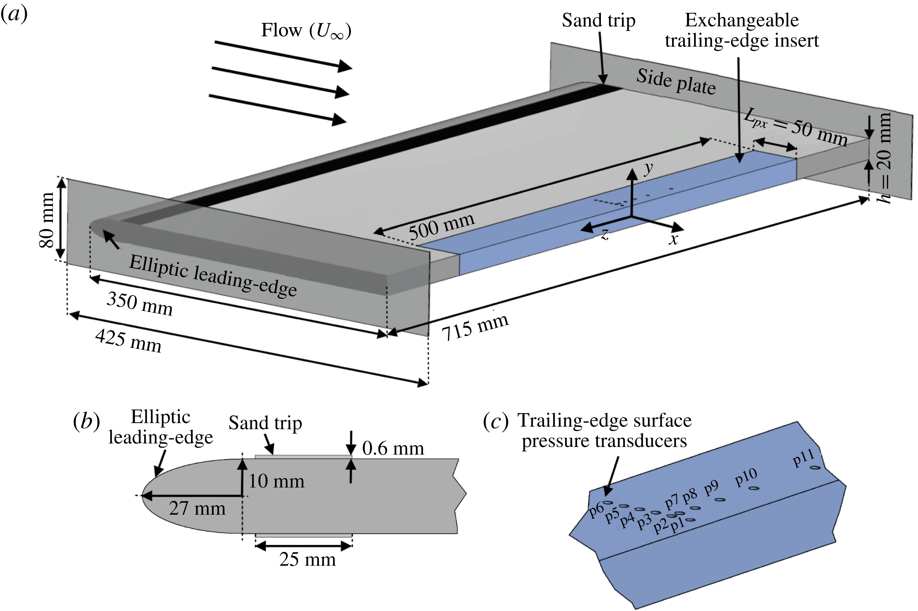
The schematic of the flat plate test rig is shown in figure 1(a). The plate has a forebody length of
 $L_{x}=350~\text{mm}$
, spanwise length of
 $L_{z}=715~\text{mm}$
and thickness of
 $h=20~\text{mm}$
. The corresponding aspect ratio of the flat plate is
 $AR_{x}=L_{x}/h=17.5$
. The model in the open-jet wind tunnel gives a blockage ratio of 1.8 %, which is expected to have a negligible effect on the results obtained (Rae & Pope Reference Rae and Pope1984). The flat plate has an elliptical leading edge with a semi-minor axis of 10 mm and a semi-major axis of 27 mm in order to prevent strong adverse pressure gradient and large leading-edge flow separation. To ensure the presence of vortex shedding, the ratio of the trailing-edge height and the boundary layer displacement thickness should obey the
 $h/\unicode[STIX]{x1D6FF}^{\ast }>0.3$
criterion, where
 $\unicode[STIX]{x1D6FF}^{\ast }$
is the boundary layer displacement thickness at the trailing edge (Blake Reference Blake2012). The bluntness ratio was found to be significantly larger than 0.3 in our experiments, ensuring the existence of vortex shedding. In order to reach a well-developed turbulent flow before the trailing-edge section, a 25 mm wide sand trip was applied just aft of the leading edge at
 $x=30~\text{mm}$
with a thickness of approximately 0.6 mm and grit roughness of 80, corresponding to the average roughness of
 $Ra=1.8~\unicode[STIX]{x03BC}\text{m}$
(Charts 2017). The trip was placed on both sides of the plate. The trailing-edge part of the plate is made as an insert, with a width (
 $L_{px}$
) and span-length of 50 mm and 500 mm, respectively, to enable tests with various trailing edges, namely solid, porous 80 PPI and porous 25 PPI, see figure 1. To ensure two-dimensional flow over the span, rectangular side plates of dimensions 425 mm by 80 mm, with sharpened leading edges with an angle of
 $20^{\circ }$
were mounted on the test apparatus. The side plates extend approximately
 $1.25h$
upstream of the leading edge and
 $2.5h$
downstream of the trailing edge. The
 $x$
-,
 $y$
- and
 $z$
-coordinates of the blunt trailing edge are taken as zero at the centre of the trailing edge. The
 $y^{\prime }$
axis is introduced on the top surface of the plate, defined as
 $y^{\prime }=y-h/2=0$
, and is used to define the boundary layer axis in § 3. The separation distance used in discussions concerning the pressure and velocity coherence and correlation studies in § 4 is denoted by
 $\unicode[STIX]{x1D709}_{x}$
,
 $\unicode[STIX]{x1D709}_{y}$
and
 $\unicode[STIX]{x1D709}_{z}$
.
(a) The schematic of a flat plate with an elliptical leading edge and exchangeable blunt trailing edge. (b) The geometry of the elliptic leading edge. (c) The position of the trailing-edge pressure transducer array.

2.2 Porous material analysis
Two metal foams with the pores per inch (PPI) of 25 and 80 have been chosen for this study. It is known from prior experimental (Ozkan, Akilli & Sahin Reference Ozkan, Akilli and Sahin2013; Ozkan & Akilli Reference Ozkan and Akilli2014) and computational (Bruneau & Mortazavi Reference Bruneau and Mortazavi2008; Liu et al.
Reference Liu, Wei and Qu2014) works that the effectiveness of porous materials as a flow control technique depends heavily on their porosity and permeability and the porous cases are, accordingly, selected to provide a wide enough porosity and permeability range. The porosity of the porous samples was measured using a Nikon XT H 320 LC computed tomography scanner and the data obtained were then visualized and analysed using the VGStudio MAX 2.2 software. The porosity (
 $\unicode[STIX]{x1D711}$
) can then be calculated from
 $\unicode[STIX]{x1D711}=V_{V}/V_{T}$
, where
 $V_{V}$
is the volume of void space and
 $V_{T}$
is the total volume of the sample. The
 $3D$
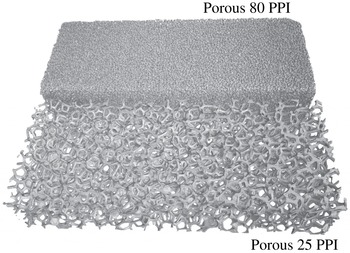
image of the two porous samples is shown in figure 2. The porosity values for the porous 25 PPI and 80 PPI samples have been found to be 90.92 % and 74.76 %, respectively.
The permeability (
 $\unicode[STIX]{x1D705}$
) of each porous material used in this study was measured using a permeability test apparatus over a wide range of Darcy velocities. The permeability rig is composed of a 2.5 m long tube, with a square cross-section, equipped with several static and dynamic pressure measurement points, with the porous sample being placed 1.2 m from the inlet. Experiments were performed on porous sample inserts of
 $80\times 80~\text{mm}$
and thickness of 10 mm. Static pressure taps were flush mounted on the inner surface of the apparatus, perpendicular to the air flow, either side of the porous sample and the pressure measurements were obtained using the MicroDaq Smart Pressure Scanner-32C. The permeability coefficient (
 $\unicode[STIX]{x1D705}$
) can then be found from the Dupuit–Forchheimer equation (Dupuit Reference Dupuit1863),
 $\unicode[STIX]{x0394}p/t=\unicode[STIX]{x1D707}/\unicode[STIX]{x1D705}\unicode[STIX]{x1D708}_{D}+\unicode[STIX]{x1D70C}C\unicode[STIX]{x1D708}_{D}^{2}$
, using the least mean squared method, where
 $\unicode[STIX]{x0394}p$
is the pressure drop across the sample,
 $t$
is the thickness of the sample,
 $\unicode[STIX]{x1D70C}$
is the density of fluid,
 $C$
is the inertial loss term,
 $\unicode[STIX]{x1D708}_{D}$
is the Darcian velocity, defined as the volume flow rate divided by cross-sectional area of the sample. The permeability values of the porous 25 PPI and 80 PPI samples were found to be
 $8.2\times 10^{-8}~\text{m}^{2}$
and
 $7.7\times 10^{-9}~\text{m}^{2}$
, respectively, implying that the 25 PPI porous medium has larger porosity and permeability coefficient than the 80 PPI sample.
Metal porous geometry obtained using X-ray computed tomographic scanning.

2.3 Force balance measurement set-up
The drag force measurements were carried out using an AMTI OR6-7-2000 force-plate unit. The flat-plate set-up was mounted on a set of steel extension arms with a symmetrical teardrop shape to minimise any additional drag forces acting on the rig. The force plate was load tested prior to the experiment. The generated voltage signal from the force plate passed through an AMTI MSA-6 strain gauge amplifier and the final data from this unit were captured using a LabView system. A detailed uncertainty and data independency test have been conducted and the sampling frequency of 45 Hz with the least uncertainty value (Theunissen et al.
Reference Theunissen, Di Sante, Riethmuller and Van den Braembussche2008) was chosen for the measurements. This sampling frequency produced the best data independency with uncertainty levels in the range of approximately 1.7–4.9 % at a 95 % confidence level. Measurements were carried out for velocities between 6 and
 $26~\text{m}~\text{s}^{-1}$
wind speed and data have been collected for 30 s at each velocity. The speeds were set such that all data were recorded once the deviation of the velocity was
 $0.2~\text{m}~\text{s}^{-1}$
or less. To ascertain the repeatability of the measurements, repeated tests were conducted and the uncertainty was found to be less than 1 %.
2.4 Hot-wire anemometry set-up
The boundary layer and wake flow measurements were carried out using single-wire Dantec 55P16 probes, with a platinum-plated tungsten wire of
 $5~\unicode[STIX]{x03BC}\text{m}$
diameter and 1.25 mm length, and cross hot-wire Dantec 55P51 probes with
 $5~\unicode[STIX]{x03BC}\text{m}$
diameter and 3 mm length platinum-plated tungsten wires. The probes were operated by a Dantec StramlinePro frame with CTA91C10 modules. The signals were low-pass filtered by the StreamlinePro frame with a corner frequency of 30 kHz before they were A/D converted, with an applied overheat ratio of 0.8 (Dantec 2013). The data have been acquired by a National Instrument 9215 type 4-channel module, with a sampling frequency of 40 kHz. The hot-wire measurements were taken for 15 s at each location. The calibration of the probes was performed using the Dantec 54H10 type calibrator. The calibration process was performed before and after each measurement and the polynomial constants were averaged prior to the post-processing of the data. The uncertainty of the measured velocity signals, obtained using the manufacturer’s method (Dantec 2013), were found to be within
 $\pm 1\,\%$
. The hot-wire probes were installed on a two-axis (
 $x$
–
 $y$
) ThorLabs LTS300M traverse system, covering a 300 mm by 300 mm domain with a typical minimum positioning accuracy of
 $\pm 5~\unicode[STIX]{x03BC}\text{m}$
.
2.5 Particle image velocimetry set-up
The particle image velocimetry (PIV) technique was used to obtain time-averaged flow quantities over the
 $x$
–
 $y$
plane. A dual-cavity laser of 200 mJ Nd:YAG with a wavelength of 532 nm was used to produce 1 mm laser sheet thickness with the time interval between each snapshot of
 $25~\unicode[STIX]{x03BC}\text{s}$
and repetition rate of 15 Hz to obtain a maximum amount of particles in the interrogation window. A mixed polyethylene glycol 80 based seeding with a particle size of
 $1{-}5~\unicode[STIX]{x03BC}\text{m}$
was used to seed the flow. A total number of 1600 image pairs were captured using a FlowSense 4 MP CCD camera with a resolution of 2072
 $\times$
2072 pixels for each case and used to compute the statistical turbulent flow quantities. The measurements were made for a field view of
 $158~\text{mm}\times 158~\text{mm}$
, which corresponds to a domain of
 $7.9~\text{h}\times 7.9~\text{h}$
in the streamwise and vertical directions. The measurements iterative process yields grid correlation window of
 $16\times 16$
pixels with an overlap of 50 %, resulting in a facial vector spacing of 0.61 mm, corresponds to the plate thickness of
 $0.031h$
.
2.6 Surface pressure measurement set-up
To achieve a better understanding of the characteristics of the boundary layer structures, surface pressure fluctuation measurements have been performed using an array of miniature Knowles FG-23329-P07 transducers, as shown in figure 1. These miniature transducers are 2.5 mm in diameter and have a circular sensing area of 0.8 mm and have regularly been used in aeroacoustic applications, particularly for boundary layer surface pressure measurements (Garcia-Sagrado & Hynes Reference Garcia-Sagrado and Hynes2012; Gruber Reference Gruber2012), due to their small size and good frequency response. It is known that at high frequencies, where the acoustic wavelength is smaller than the transducer sensing area, the measurement errors may arise due to the spatial integration of the pressure fluctuations (Corcos Reference Corcos1963). In order to eliminate the errors present in the wall pressure spectrum measurement, a small-sized pinhole transducer sensing area is employed. The trailing-edge section of the rig is instrumented with 11 flush mounted miniature Knowles transducers under a pinhole mask of 0.4 mm diameter. According to the studies carried out by Gravante et al. (Reference Gravante, Naguib, Wark and Nagib1998), to avoid attenuation due to the pinhole size, the pinhole non-dimensional diameter (
 $d^{+}=du_{\unicode[STIX]{x1D70F}}/\unicode[STIX]{x1D708}$
) should be in the range of
 $12<d^{+}<18$
for frequencies up to
 $f^{+}=f\unicode[STIX]{x1D708}/u_{\unicode[STIX]{x1D70F}}^{2}=1$
. The pinhole diameter (
 $d$
) to the wall unit
 $\unicode[STIX]{x1D708}/u_{\unicode[STIX]{x1D70F}}$
ratio, i.e.
 $d^{+}=du_{\unicode[STIX]{x1D70F}}/\unicode[STIX]{x1D708}$
, determines the significance of the pressure fluctuations attenuation. The pinhole mask used for the current study for the free-stream velocity of
 $20~\text{m}~\text{s}^{-1}$
, gives a non-dimensionalized diameter range of
 $12<d^{+}<19$
, which is close to the pinhole diameter suggested by Gravante et al. (Reference Gravante, Naguib, Wark and Nagib1998). The uncertainty obtained from the surface pressure measurements were found to be within
 $\pm$
0.5 dB with 99 % of confidence level. The data have been acquired using a National Instrument PXle-4499, with a sampling frequency of
 $2^{16}~\text{Hz}$
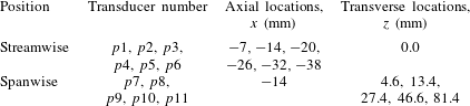
and measurement time of 32 s. The transducers are arranged in the form of an L-shaped array in the streamwise and spanwise directions (see figure 1). The transducers located in the spanwise direction are used for the calculation of the spanwise coherence and length scale of boundary layer structures, while the transducers employed in the streamwise direction provide information on the evolution of the turbulence structures as they move downstream towards the trailing edge and their convection velocity. The detailed locations of the pressure transducers on the detachable trailing-edge part are shown in figure 1(c) and summarized in table 1. The pressure transducers,
 $p2$
to
 $p6$
, are equally spaced in the streamwise direction, while the transducers,
 $p7$
to
 $p11$
, are placed 14 mm upstream of the trailing edge and are spaced unequally in the spanwise direction to maximize the number of correlation distance combinations (
 $\unicode[STIX]{x1D709}_{z}$
) between the transducers in order to obtain more accurate results over the whole frequency range.
Positions of the pinhole transducers upstream of the trailing edge.

3 Aerodynamic and flow-field analysis
3.1 Steady drag coefficient
A basic but fundamental understanding of the problem can be gained by studying the aerodynamic forces acting on the plate. The steady aerodynamic force measurement of the blunt flat plate with solid and porous trailing edges are presented and explained in this subsection. The experiments covered a wide range of flow velocities,
 $U_{\infty }=6$
–
 $26~\text{m}~\text{s}^{-1}$
, corresponding to the Reynolds numbers of
 $Re_{L_{x}}=1.4\times 10^{5}$
–
 $6.0\times 10^{5}$
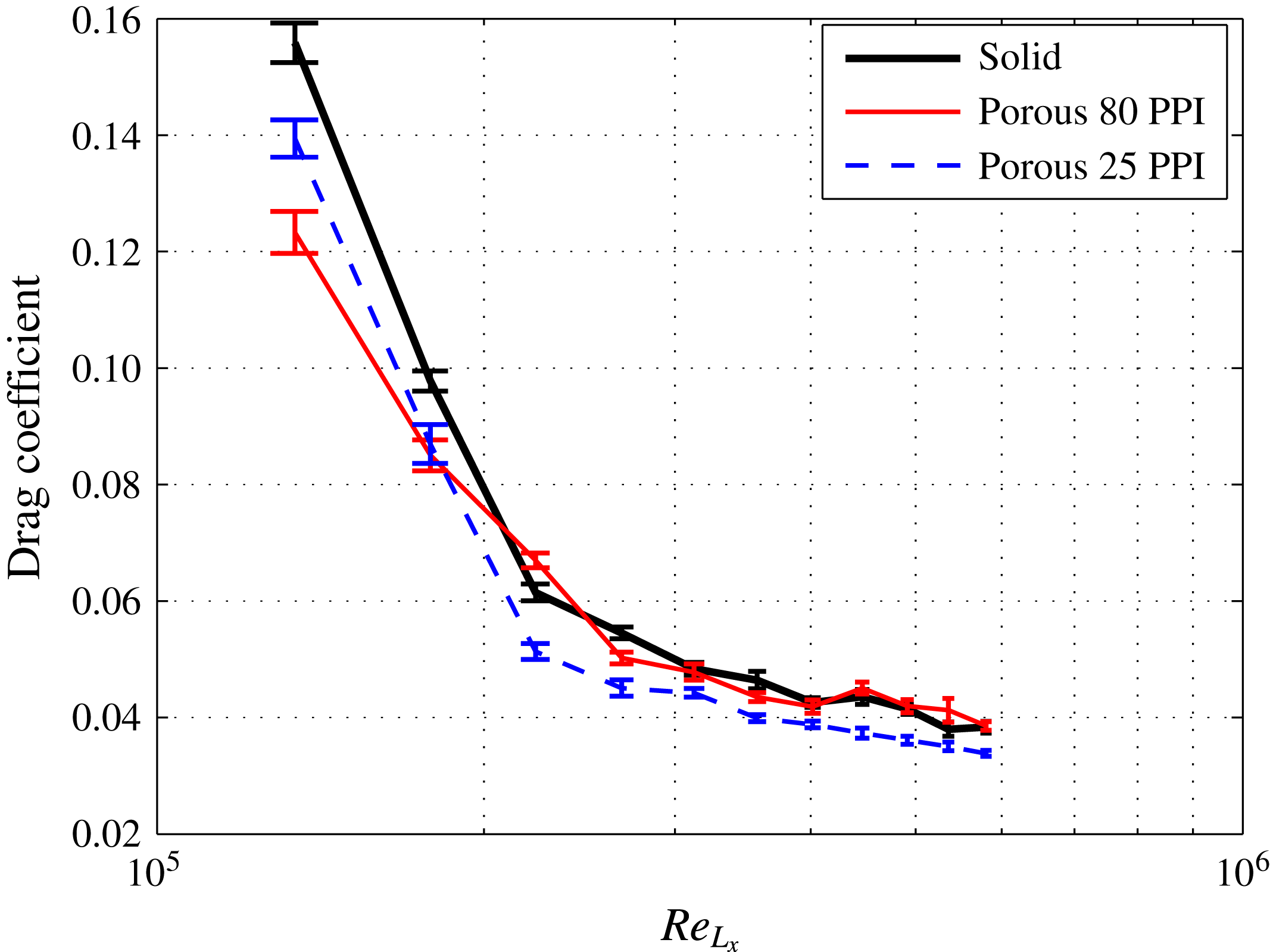
. The results presented in figure 3 show the drag coefficient (
 $C_{D}$
) of the plate against the Reynolds number for the solid and porous trailing edges. The drag coefficient (
 $C_{D}$
) is calculated as
 $C_{D}=F_{x}/(0.5\unicode[STIX]{x1D70C}U_{\infty }^{2}A)$
, where
 $F_{x}$
is the force acting on the plate in the streamwise direction and
 $A$
is the plate plan view area. The vertical error bars centred on the
 $C_{D}$
mean values denote the estimated
 $C_{D}$
uncertainty with 95 % confidence level.
Results have shown that the use of porous treatment can significantly reduce the drag force. The results for the solid case have shown that the drag coefficient experiences a sudden sharp drop at low
 $Re_{L_{x}}$
and gradually reaches an area of almost
 $Re_{L_{x}}$
independency at higher Reynolds numbers. The sudden decrease in the drag coefficient behaviour at low Reynolds number and the variation in drag, covering an almost one decade of
 $Re_{L_{x}}$
, can potentially be due to the laminar to turbulence transition phenomena (Eiffel Reference Eiffel1912). This, however, needs further experimental and numerical investigations. It can also be seen that the use of 25 PPI porous material leads to the reduction of
 $C_{D}$
by up to 16 % compared to the solid case. The trends observed from the solid and 80 PPI porous cases are almost identical at high Reynolds numbers, indicating that the boundary layer and wake flows at high Reynolds numbers behave similarly in the case of 80 PPI and solid trailing edges. This behaviour can be explained by the fact that for the porous medium with low permeability, a longer flow and porous surface interaction is needed to enable flow penetration into the porous medium. Therefore, the porous materials with high PPI and low permeability behave more or less like the solid case. The significant reduction obtained for the case of 25 PPI can be attributed to the flow penetration into the pores, flow discharge into the wake and attenuation of the vortex shedding from the trailing edge, which will be further discussed in §§ 3.2 and 3.3.
The measured drag coefficient for the flat plate with different trailing edges.

3.2 Trailing-edge flow field
In order to better understand the effects of the porous trailing edge on the boundary layer structures, wake development and vortex shedding, measurements have been performed using PIV and hot-wire anemometry at the flow velocity of
 $U_{\infty }=20~\text{m}~\text{s}^{-1}$
, corresponding to the Reynolds number of
 $Re_{L_{x}}=4.6\times 10^{5}$
. Figure 4 illustrates the time-averaged normalized streamwise (
 $U$
) and vertical (
 $V$
) velocity components for the blunt trailing edge with and without porous treatment. The categorization of vortex shedding regimes in the wake velocity profile specifically in the near-wake flow can be assessed by looking into the vortex formation length and the vortex cores (mean recirculation) region. The non-dimensionalized vortex formation length (
 $L_{f}/h$
) is defined as the distance between the trailing edge and the end of the vortex region, where the maximum streamwise velocity fluctuations are obtained, while the non-dimensionalized vortex cores region (
 $x_{vc}/h$
) corresponds to the position of the recirculation core (Williamson Reference Williamson1996).
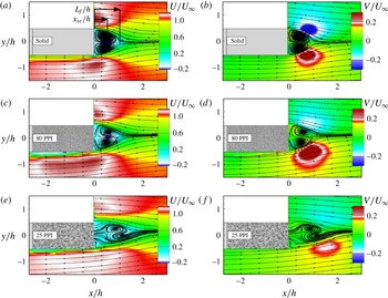
Time-averaged flow pattern for normalized streamwise (
 $U$
) and vertical (
 $V$
) velocity components for solid (a,b), porous 80 PPI (c,d) and 25 PPI (e,f).

The respective
 $L_{f}/h$
and
 $x_{vc}/h$
locations are illustrated in figure 4(a). Results in figure 4(a,b) show that the flow recirculation behind the solid trailing edge occurs within
 $0.05\lesssim x/h\lesssim 1.04$
, with a pair of counter-rotating vortices formed in the very near wake with identical symmetric vortex core structure with respect to the centreline of the trailing edge. The results for the porous medium with low permeability (80 PPI) shows a small shift in the location of the recirculation region, see figure 4(c,d), with the recirculation occurring within
 $0.15\lesssim x/h\lesssim 1.06$
. It can also be seen that the counter-rotating vortices formed are nearly symmetric, with a slight shift between the two vortex cores. The use of the porous 25 PPI with higher permeability value, however, leads to significant changes to the vortex core structure and the location of the recirculation zone. This can be seen in figure 4(e,f) that the recirculation area has moved further downstream to
 $0.5\lesssim x/h\lesssim 1.8$
. The
 $L_{f}/h$
and
 $x_{vc}/h$
for the solid, porous 80 PPI and porous 25 PPI trailing edges have been found to be 1.04, 1.06 and 1.8, and 0.4, 0.64 and 1.2, respectively, indicating a significant delay in the formation of the vortex shedding due to interaction of flow with the porous treatment. The delay in the formation of the vortex shedding is consistent with the observations in figure 3, i.e. drag reduction using porous treatment. A similar observation was made by Bearman & Tombazis (Reference Bearman and Tombazis1993), where they had shown the use of wavy blunt trailing edge can lead to changes to the length of the recirculation region (
 $L_{f}$
), recovery of the base pressure and reduction of drag.
Another interesting feature observed in figure 4 is the emergence of an area of flow acceleration over the trailing-edge region due to the pressure difference at the trailing edge. This effect can also be primarily related to the development of the core of a vortex, which in general imposed by a minimum pressure (low-pressure vortex). The low pressure in the vortex core against the high-pressure outside the vortex core creates a partial vacuum (suction), enabling flow to be accelerated near the trailing edge. The flow acceleration region of the
 $U$
-components can be seen within
 $-1\lesssim x/h\lesssim 0.5$
and
 $-1.3\lesssim y/h\lesssim -0.5$
for the case of solid trailing edge (figure 4
a), followed by a rapid vertical flow movement, i.e. velocity overshoot near the trailing edge, leading to the flow recirculation in the near-wake region. Similar observations can be made in the case of porous 80 PPI (figure 4
c) with a broader flow acceleration region and less strong compared to that of the solid case. However, unlike the solid trailing edge, porous 25 PPI exhibits a much more streamlined behaviour, with a much lower flow acceleration upstream of the trailing edge and reduced velocity overshoot over the blunt trailing edge. Results have also shown that the acceleration region of the
 $V$
-component for the porous 25 PPI in the wake has moved even further downstream compared to the solid and 80 PPI cases. The significant changes observed for the porous 25 PPI trailing edge is believed to be due to the penetration of the boundary flow into the porous medium, creation of an internal hydrodynamic field and discharge of the flow into the wake region. These phenomena will be further discussed in §§ 3.4 and 3.5.
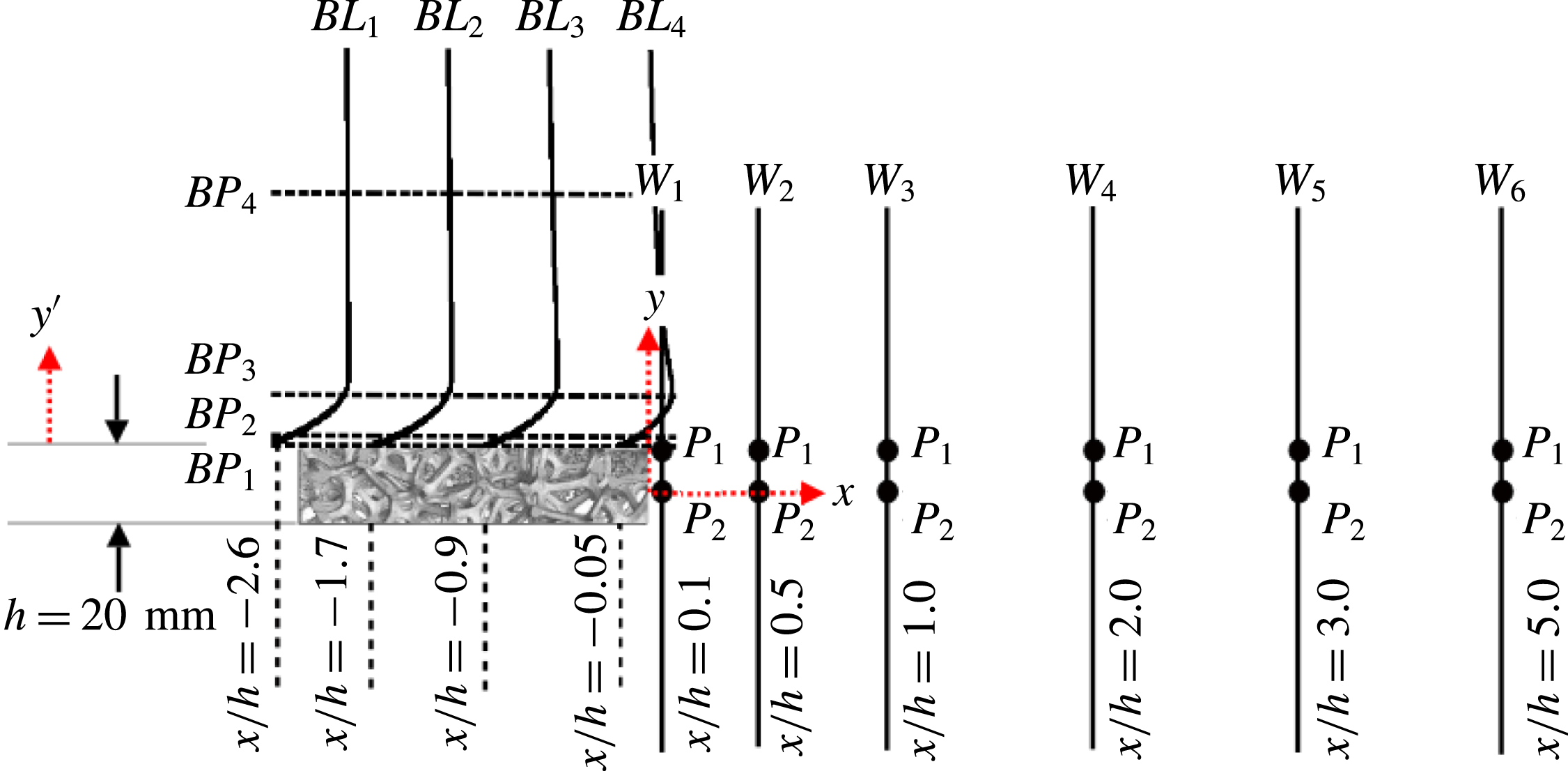
The schematic of the blunt trailing-edge rig and the position of the hot-wire for boundary layer (
 $BL_{i}$
) and wake (
 $W_{i}$
) measurements.

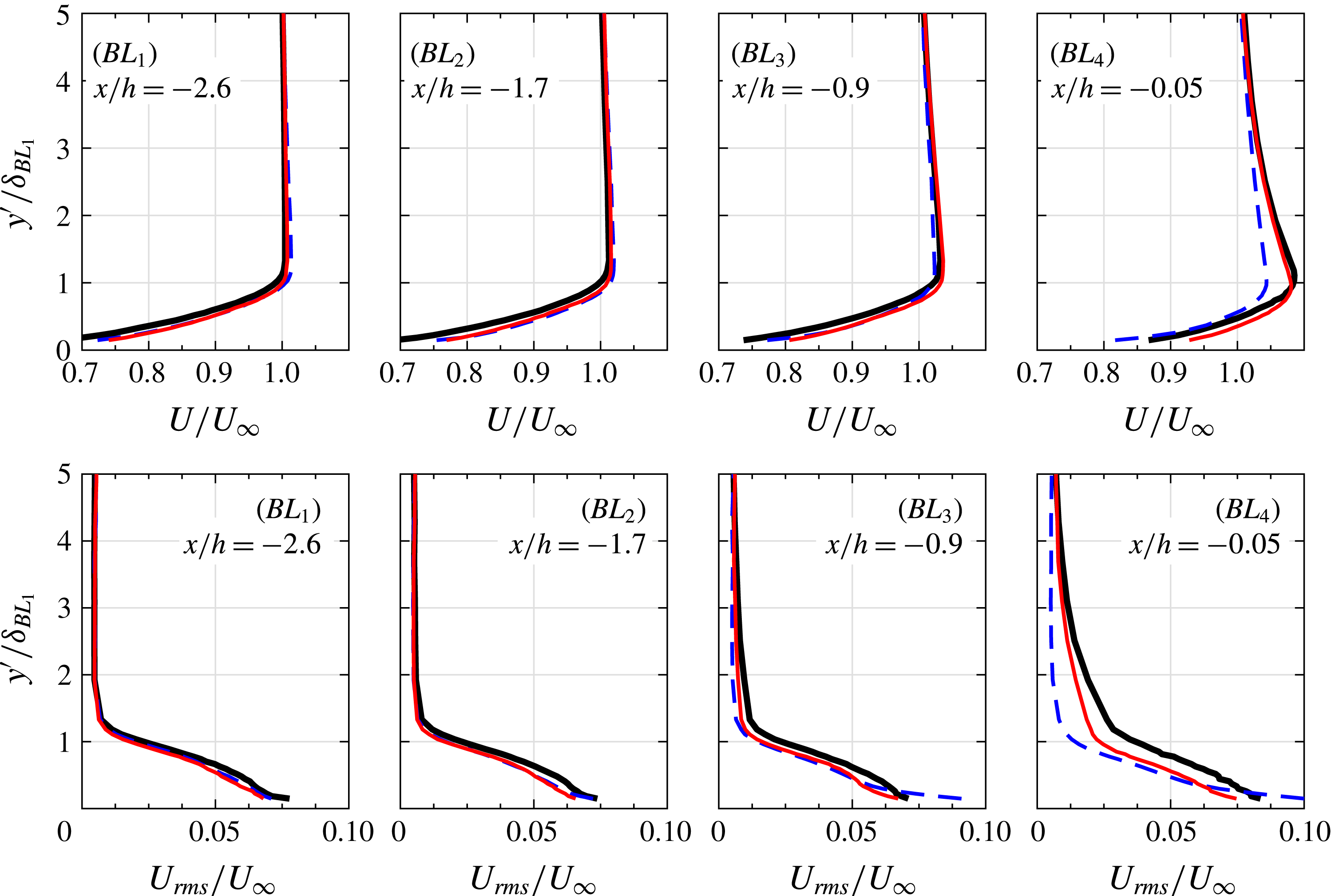
Boundary layer mean and r.m.s. velocity profiles at different streamwise locations upstream of the trailing edge. Solid trailing edge (——), porous 80 PPI trailing edge (——), porous 25 PPI trailing edge (- - -).

Figure 6 presents the mean and root-mean-square (r.m.s.) boundary layer velocity profiles along the boundary layer (
 $BL$
) lines shown in figure 5. The measurements were conducted at the flow velocity of
 $U_{\infty }=20~\text{m}~\text{s}^{-1}$
using a single hot-wire probe and the data have been collected between
 $y^{\prime }/h\approx 0$
and
 $y^{\prime }/h=2.5$
at 35 stations above the plate for each line, where
 $y^{\prime }=0$
is the plate top surface, as defined in § 2.1. The distance from the surface (
 $y^{\prime }$
-axis) has been normalized by the boundary layer thickness at
 $BL_{1}$
,
 $x/h=-2.6$
, upstream of the exchangeable trailing-edge part. Note that at
 $BL_{1}$
, the flow velocity approaches to zero at the solid surface, i.e. the no-slip condition, which will not be the case over the porous surface due to the flow penetration into the porous medium (Berg et al.
Reference Berg, Cense, Hofman and Smits2007). The boundary layer velocity results show that there is an increase in the velocity gradient at the wall from
 $BL_{1}$
to
 $BL_{4}$
, which implies the presence of a favourable pressure gradient flow upstream of the trailing edge, which will eventually cause strong flow acceleration over the trailing edge (Abernathy Reference Abernathy1970). The velocity profiles for the solid trailing edge downstream of
 $BL_{1}$
gradually deviate from that of a standard turbulent boundary layer profile as a result of the bluntness effects, with a clear velocity overshoot, signifying the presence of flow acceleration in the trailing-edge region. The peak of the velocity overshoot occurs at
 $y^{\prime }/\unicode[STIX]{x1D6FF}_{BL_{1}}=1$
and does not change greatly with
 $x/h$
. The r.m.s. velocity results clearly show that the solid trailing edge exhibits a larger level of velocity fluctuations than the porous cases, almost in the whole boundary layer region. In the case of the 80 PPI trailing edge, the boundary layer profiles observed at all the measurement locations are very similar to that of the solid trailing-edge case, but with slightly milder velocity overshoot in the vicinity of the trailing edge. It is also noticed that the use of porous 80 PPI treatment reduces the r.m.s. velocity value over a large part of the boundary layer compared to the solid trailing edge. The results obtained for the flat plate with the porous 25 PPI treatment show that the flow is more streamlined over the trailing edge and it experiences much less acceleration and therefore less velocity overshoot in the trailing-edge region. The r.m.s. velocity results in the case of 25 PPI trailing edge changes rather abruptly over a large part of the boundary layer, particularly in the boundary layer outer regions. This becomes clearly visible at
 $x/h=-0.9$
(
 $BL_{3}$
) and
 $x/h=-0.05$
(
 $BL_{4}$
), upstream of the trailing edge, where the flow acceleration was observed for the solid trailing edge. However, there is an increase in the r.m.s. velocity magnitude near the wall region for the case of porous 25 PPI at both
 $BL_{3}$
and
 $BL_{4}$
. Despite the significant reduction of
 $U_{rms}$
over a large part of the boundary layer, the use of the 25 PPI material is shown to increase the energy content of the velocity fluctuations over a small region in the vicinity of the porous surface, which can be attributed to the frictional forces at the surface of the porous material. This is particularly an interesting result as it shows that the energy content of the large coherent structures in the log law and outer layer regions, mainly responsible for the low frequency surface pressure fluctuations and the trailing-edge noise generation (Garcia-Sagrado & Hynes Reference Garcia-Sagrado and Hynes2012) can be significantly reduced using porous treatments.
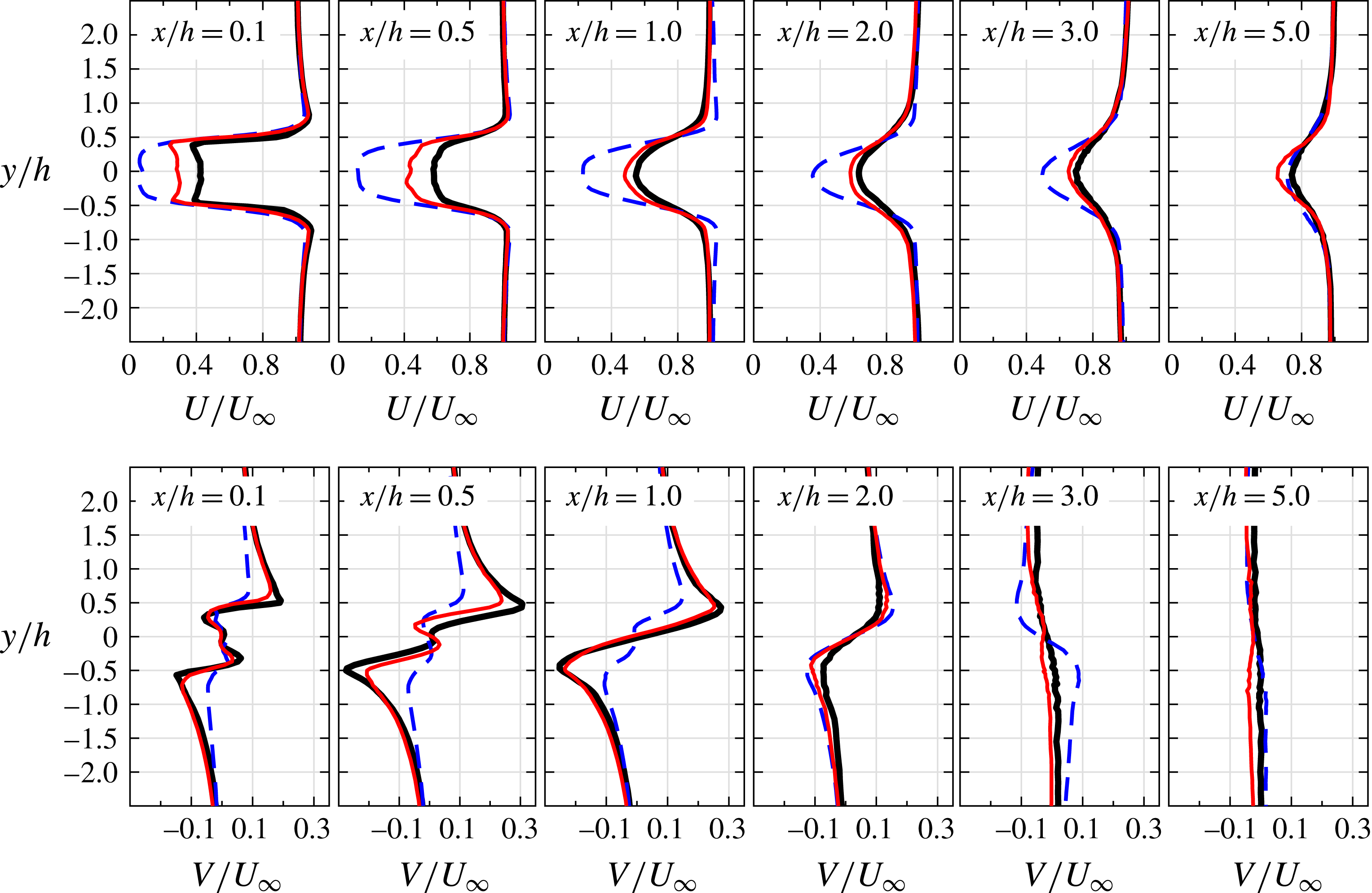
Mean streamwise (
 $U$
) and vertical (
 $V$
) velocity components in the wake of the blunt trailing edge. Solid trailing edge (——), porous 80 PPI trailing edge (——), porous 25 PPI trailing edge (- - -).

Figure 7 shows the streamwise (
 $U$
) and vertical (
 $V$
) velocity profiles at different axial locations, namely
 $x/h=0.1$
, 0.5, 1.0, 2.0, 3.0 and 5.0 downstream of the trailing edge (see figure 5), covering a wide range of near- to far-wake locations. Note that the measurements have been carried out using hot-wire anemometry and therefore, the streamwise velocity component is always positive, i.e. showing the absolute value of the velocity. The actual value of the
 $U$
-component can be found in figure 4. It is clear from the results that the porous treatments can significantly change the flow structure in the near-wake region. Results show that both the porous cases significantly reduce the magnitude of the streamwise velocity in the near wake. The
 $U$
-component velocity profiles show that the porous treatments delay the formation of vortex shedding in the wake, i.e. near-wake stabilization, which is consistent with the streamline flow pattern observed in figure 4.
On the other hand, the large deficit observed in the case of 25 PPI is due to the suppression of the recirculation region and reduction of the velocity overshoot over the trailing edge, resulting in a more streamlined flow over the trailing edge and larger deficit in the plate near-wake region. The porous material restraint the entrainment of the high momentum fluid from the free stream into the wake field, which causes lower momentum transfer in the wake and results in larger velocity deficit in the plate near-wake region. The reduced impact of vortex shedding due to the delayed recirculation also enhances the effect of the base pressure recovery in the wake, which in turn, leads to the reduction in
 $C_{D}$
. The drag associated with the vortex shedding can be obtained using the wake velocity deficit information. In order to calculate the drag force using the wake velocity results (
 $C_{D_{W}}$
), the methodology described by Naghib-Lahouti, Hangan & Lavoie (Reference Naghib-Lahouti, Hangan and Lavoie2015) has been adopted as follows,
 $$\begin{eqnarray}C_{D_{W}}=\frac{2}{A}\int \frac{U}{U_{\infty }}\left(1-\frac{U}{U_{\infty }}\right)\text{d}y+\frac{2}{A}\int \left(\frac{U_{rms}}{U_{\infty }}\right)^{2}\text{d}y,\end{eqnarray}$$
where
 $A$
is the plate plan view area and the integral must be carried out outside the vortex recirculation region in the near-wake area. The two integrals in (3.1) are estimated based on the streamwise mean and fluctuating velocity components. In the present study, these terms are calculated based on the velocity quantities located at
 $x/h=2$
, downstream of the trailing edge. The trend of the total drag estimated from the wake
 $C_{D_{W}}$
, at a flow velocity of
 $U_{\infty }=20~\text{m}~\text{s}^{-1}$
, corresponding to the Reynolds number of
 $Re_{L_{x}}=4.6\times 10^{5}$
, is consistent with the drag coefficient
 $C_{D}$
results found using the force balance measurements. The results show that a significant reduction of the total drag
 $C_{D_{W}}$
can be achieved in the case of porous 25 PPI trailing edge, with a reduction of
 ${\approx}$
15 %, relative to that of the solid case, which is in agreement with the drag reduction obtained in figure 3. The
 $V$
-velocity component results show a different behaviour than the
 $U$
-velocity component. The vertical velocity component in the near wake can be linked to the vortex formation and roll-up mechanism. The
 $V$
-velocity results for the solid trailing edge at
 $x/h=0.1$
show the existence of a secondary small recirculation area near the centreline (
 $y=0$
) and two larger recirculation areas nearer to the trailing edge. The small recirculation near the centreline disappears quickly further downstream, leading to only one large recirculation area, ending between
 $x/h=2.0$
and
 $3.0$
. The
 $V$
-component velocity profiles observed for the 80 PPI trailing edge is very similar to that of the solid trailing edge, but the 25 PPI trailing edge exhibits a very different behaviour. The main recirculation area of the 25 PPI case is much weaker than the solid case, indicating the stabilization of the shear layer and delay of the vortex shedding formation. The energy content of the boundary layer and wake structures will be further discussed in figures 8 and 11.
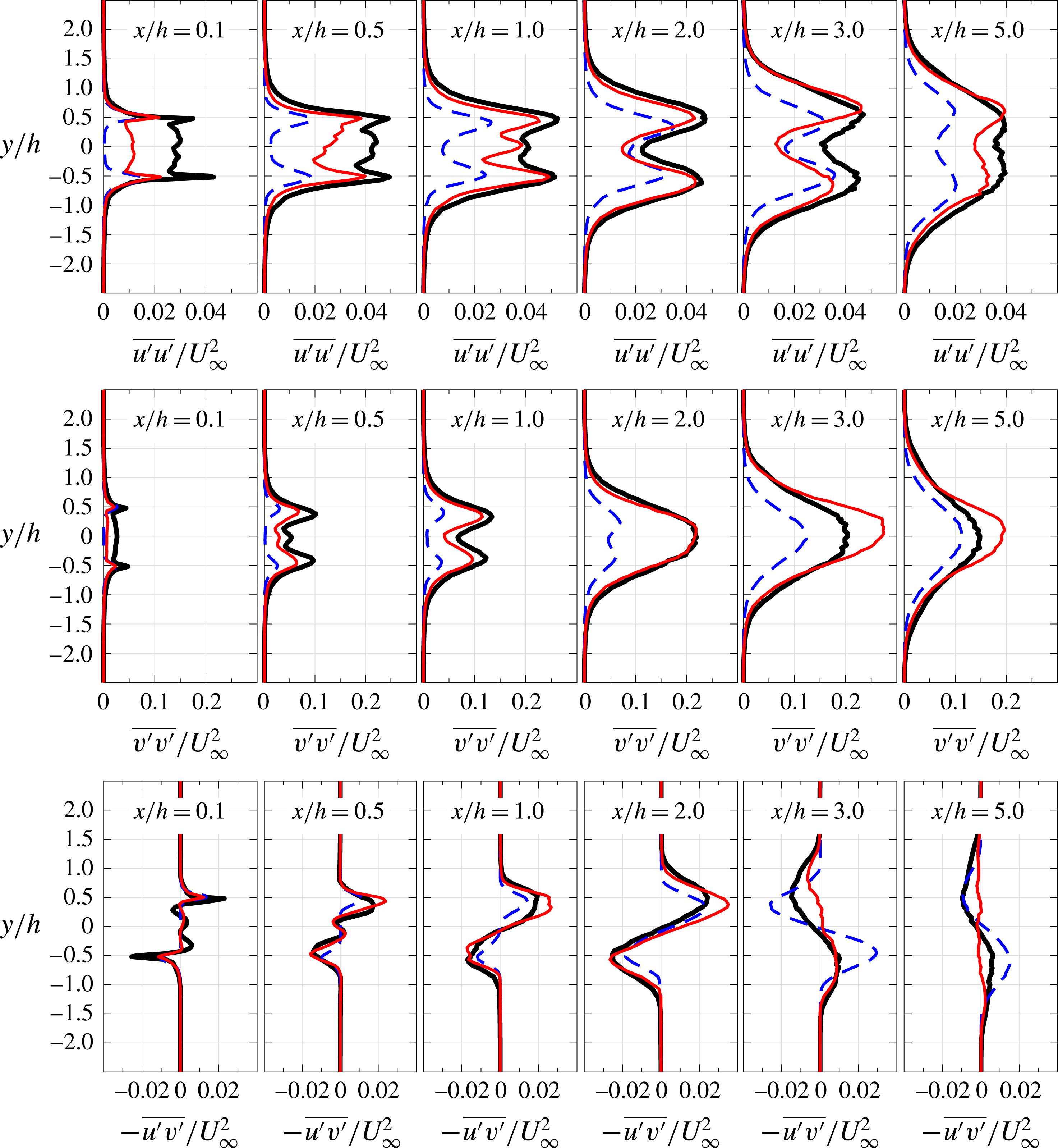
Figure 8 presents the normalized Reynolds normal stress (
 $\overline{u^{\prime }u^{\prime }}/U_{\infty }^{2}$
,
 $\overline{v^{\prime }v^{\prime }}/U_{\infty }^{2}$
) and shear stress (
 $-\overline{u^{\prime }v^{\prime }}/U_{\infty }^{2}$
) components within the wake at
 $x/h=0.1$
, 0.5, 1.0, 2.0, 3.0 and 5.0. It is clear from the figure that the Reynolds stresses are symmetrical about the wake centreline for all cases and peak at about the trailing-edge lip-line location
 $y/h=\pm 0.5$
. The near-wake results show that the use of porous trailing edge can lead to significant reduction of the normal and shear stress terms along the centreline to almost zero and also considerable reduction at the peak location (
 $y/h=\pm 0.5$
). Results have also shown that the use of porous trailing edge leads to a considerable reduction of the wake width in the
 $y$
-direction at
 $x/h=3.0$
and
 $5.0$
. A noticeable difference between the magnitude of the
 $\overline{u^{\prime }u^{\prime }}$
and
 $\overline{v^{\prime }v^{\prime }}$
normal stress components can be observed in the
 $x/h\gtrsim 0.5$
region, where is dominated by the flow recirculation in the case of the solid or delayed vortex shedding for the porous trailing-edge cases. The results obtained for the solid and porous trailing edges show that the
 $\overline{v^{\prime }v^{\prime }}$
component can become twice, or more, as large as the
 $\overline{u^{\prime }u^{\prime }}$
at the downstream locations (
 $x/h\gtrsim 0.5$
). The increase in the
 $v$
-fluctuations indicates the presence of large swirling turbulent structures, i.e. the formation of vortex shedding (Bevilaqua Reference Bevilaqua1975). Also, this suggests the existence of a highly anisotropic flow at these locations due to the vortex formation.
Reynolds stress components within the wake. Solid trailing edge (——), porous 80 PPI trailing edge (——), porous 25 PPI trailing edge (- - -).

The anisotropy level
 $\unicode[STIX]{x1D623}_{ij}$
can be estimated from the Reynolds stress anisotropy tensor,
 $\unicode[STIX]{x1D623}_{ij}=\unicode[STIX]{x1D619}_{ij}/2K-\unicode[STIX]{x1D6FF}_{ij}/3$
, where
 $\unicode[STIX]{x1D619}_{ij}$
is the Reynolds stress term,
 $K=1/2\unicode[STIX]{x1D619}_{ii}$
is the turbulent kinetic energy and
 $\unicode[STIX]{x1D6FF}_{ij}$
is the Kronecker delta function. The overall turbulence anisotropy state can be evaluated by using the second II (
 $-\unicode[STIX]{x1D623}_{ij}\unicode[STIX]{x1D623}_{ji}/2$
) and third III (
 $\unicode[STIX]{x1D623}_{ij}\unicode[STIX]{x1D623}_{jk}\unicode[STIX]{x1D623}_{ki}/3$
) nonlinear principal invariants of
 $\unicode[STIX]{x1D623}_{ij}$
(Lumley Reference Lumley1979), where II indicates the degree of anisotropy and III represents the anisotropy nature (Oyewola, Djenidi & Antonia Reference Oyewola, Djenidi and Antonia2004). The anisotropy invariant maps (AIMs) of the Reynolds stress components at all wake locations (
 $0.1\leqslant x/h\leqslant 5.0$
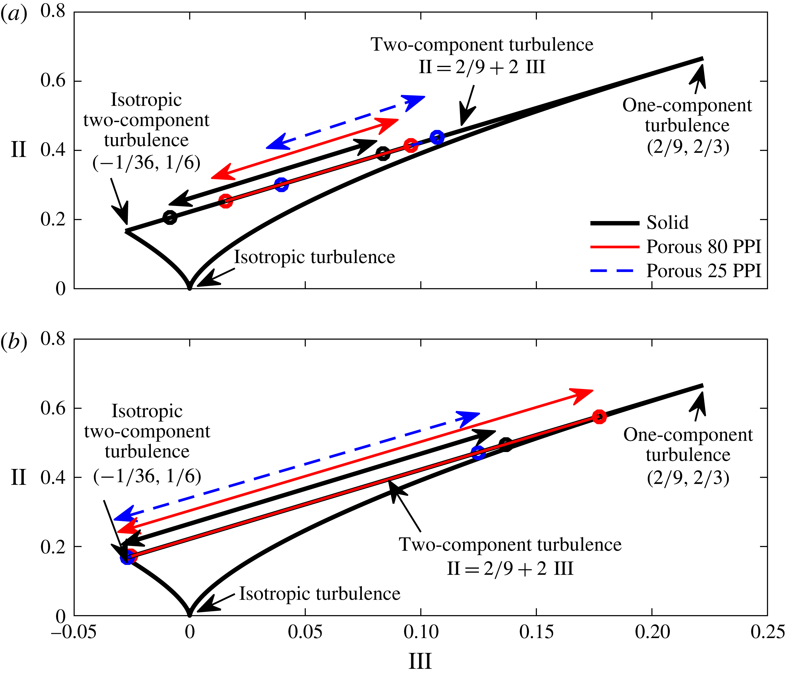
) downstream of the trailing-edge lip line and along the centreline, with a cross-plot of II versus III are summarized in figure 9. The turbulence state of the Reynolds stress components is depicted by the boundaries of the AIM. As only the streamwise
 $U$
and vertical
 $V$
velocity components are available from the present hot-wire measurements, all the data are gathered over the two-component turbulence state at the upper boundary line of the AIM (i.e.
 $\text{II}=2/9+2\text{III}$
or
 $b_{13}=b_{23}=0$
). This is an acceptable assumption as the wake flow is predominantly two-dimensional, i.e.
 $W\approx 0$
. Figure 9(a) shows that the Reynolds stress components of the wake structures in the case of the porous 25 PPI and 80 PPI at the trailing-edge lip line gradually separate from the isotropic two-component turbulence state and move towards a one-component turbulence state. At the trailing-edge centreline, figure 9(b) shows that the Reynolds stress components of all cases are nearly in an isotropic two-dimensional (2-D) turbulence state, which implies that the turbulent kinetic energy tends to be equally distributed among the two velocity components and distinctly tend towards the one-dimensional (1-D) turbulence state, especially for the case of porous 80 PPI.
Anisotropy invariant map (AIM) of Reynolds stress tensor at several wake locations downstream of the (a) trailing-edge lip line and (b) trailing-edge centreline. The arrows show the range of anisotropy variation for flow measurements over
 $0.1\leqslant x/h\leqslant 5.0$
.

In addition to the normal Reynolds stress terms, studying the shear stress terms helps better understand the energy production within the turbulent media and the mechanisms governing the stabilization of the Tollmien–Schlichting instabilities (Bushnell & Hefner Reference Bushnell and Hefner1990). It is, therefore, important to study the Reynolds shear stress component (
 $-\overline{u^{\prime }v^{\prime }}/U_{\infty }^{2}$
) for both solid and porous trailing-edge cases within the wake region, see figure 8. The results at each location display a symmetrical distribution of shear stress along the wake centreline. It is clear that the shear stress is reduced significantly within
 $x/h=0.1$
–2.0 due to the larger momentum deficit in the case of 25 PPI. Also, the lower peaks in the case of 25 PPI trailing edge compared to the solid trailing edge is due to the elongation of the wake region and the attenuation of vortex shedding in the trailing-edge area, as discussed earlier for figure 7. In contrast, the distribution of
 $-\overline{u^{\prime }v^{\prime }}$
obtained at
 $x/h=3.0$
and
 $x/h=5.0$
shows a slight increase in the peak magnitude in the porous 25 PPI case, which indicates the presence of a delayed vortical structure in this region, as observed in figure 4.
3.3 Velocity power spectra in the boundary layer and wake
The dominant turbulent structures within the boundary layer and their frequency–energy content can be studied using the velocity power spectrum (
 $\unicode[STIX]{x1D719}_{uu}$
). Figure 10 presents the velocity power spectral density (PSD) as a function of the Strouhal number (
 $St=fh/U_{\infty }$
) at different axial locations upstream of the trailing edge and provides a comparison between the three investigated trailing-edge cases. In order to estimate the energy content at different frequencies, the Welch’s power spectral density of velocity fluctuations (
 $\unicode[STIX]{x1D719}_{uu}$
) has been performed based on the time-domain hot-wire data using Hamming windowing for segments of equal length with 50 % overlap. The frequency resolution (
 $\unicode[STIX]{x0394}f$
) was set to 64 Hz and the frequency wavelength was equal to
 $1/5$
of the window length used in the windowing process. The velocity fluctuation energy power spectrum at
 $BP_{1}$
corresponds to the point near the surface (
 $y^{\prime }/h=0.025$
), while
 $BP_{2{-}3}$
, i.e. the top two rows, show the results further away from the wall regions of the boundary layer at
 $y^{\prime }/h=0.075$
and 0.33 (velocity overshoot location). Results have shown that in the vicinity of the wall of the porous treatment, especially in the case of 25 PPI, causes an increase in the energy content over the whole Strouhal range. This is believed to be, to some extent, due to the increased level of frictional forces acting on the flow near the surface (
 $BP_{1}$
), which is also in agreement with the r.m.s. velocity results presented in figure 6. It can also be seen that the level of such frictional forces increases with the flow travelling downstream over the porous section. The investigated spectra at the velocity overshoot location (
 $BP_{3},BL_{2{-}4}$
) clearly show that the overall energy content of the boundary layer structures reduces significantly as a result of the boundary layer interaction with the porous surface. The results for the solid trailing edge also show a strong tonal behaviour at
 $St\approx 0.21$
, which can be attributed to the presence of a strong hydrodynamic field travelling upstream from the wake region, where flow recirculation occurs. This tonal peak energy has been detected at almost all locations, which is also visible in the case of porous 80 PPI shown in figure 10, except for regions far upstream of the trailing edge and very close to the surface. Interestingly, in the vicinity of the trailing edge at
 $BL_{3{-}4}$
results show that the use of 25 PPI porous material results in the complete suppression of the tonal peak and the emergence of a small broadband hump between
 $St=0.3$
and
 $0.9$
at
 $BP_{3},BL_{4}$
. The broadband hump region is shown in plots (g,h) with a thick line. While the near-wall frictional forces result in an overall increase in the energy content of the flow over the entire frequency range, the increase over a small frequency band (
 $St=0.3$
–0.9) seems to be due to a different mechanism. This is believed to be due to the presence of a strong hydrodynamic field inside the porous medium, which will be discussed further in § 3.5 and proven using various pressure and velocity correlation and coherence studies. This phenomenon can also be seen in the near-wake velocity frequency–energy content and the surface pressure fluctuations (
 $\unicode[STIX]{x1D719}_{pp}$
) results in figures 11 and 13. From the velocity PSD results presented in figure 10, it can, therefore, be concluded that the use of porous treatments can lead to significant reduction of the energy content of the large turbulent structures within the boundary layer and the suppression of the vortex shedding tonal peaks. Understanding of the mechanisms through which the porous treatment causes such changes requires more in-depth analysis of the boundary layer surface pressure fluctuations, which will be dealt with in §§ 3.4, 3.5 and 5.
The velocity power spectral density at different locations in the boundary layer. Solid trailing edge (——), porous 80 PPI trailing edge (——), porous 25 PPI trailing edge (- - -).

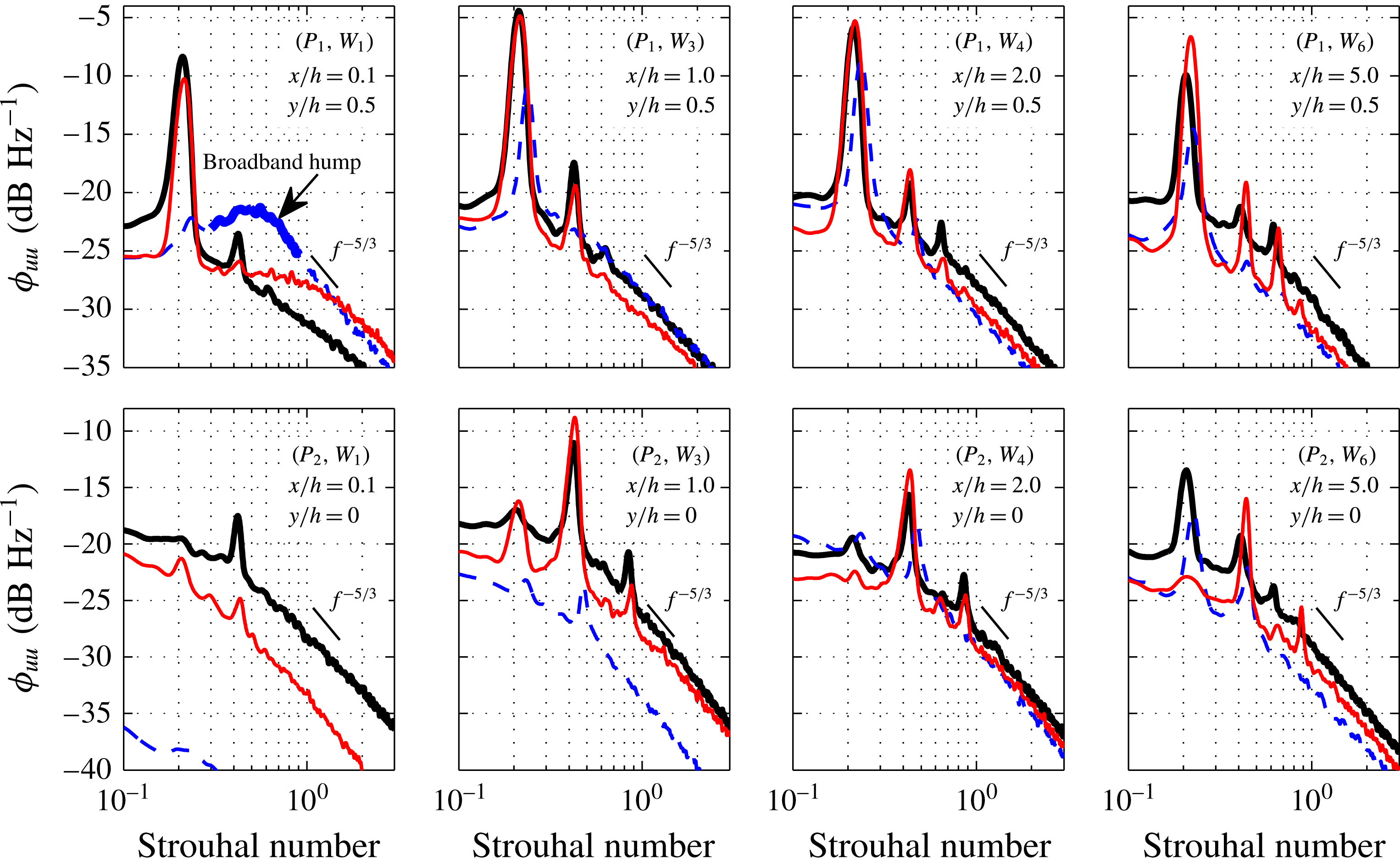
To properly understand the properties of the wake turbulence structures, one needs to study their energy–frequency content, as well as the basic velocity and turbulent kinetic energy profiles. The results of the power spectral density (PSD) analysis of the wake flow velocity (
 $\unicode[STIX]{x1D719}_{uu}$
) are presented at several wake locations downstream of the trailing-edge, along the lip line (
 $y/h=0.5$
) and along the centreline (
 $y/h=0$
), see figure 11. The measurement locations are shown in figure 5. The fundamental, first and second harmonics of the vortex shedding frequency can be clearly seen from the results of the solid trailing edge. The slope of the velocity spectra after the second harmonic (
 $St=0.6$
) for all downstream locations appears close to
 $f^{-5/3}$
. The results show a significant and consistent reduction of the broadband content of
 $\unicode[STIX]{x1D719}_{uu}$
for both porous cases. In the case of the porous 80 PPI, as mentioned before, the treatment is unable to change the tonal characteristics of the flow structures. However, the reduction in the broadband content of the energy spectra in the case of 80 PPI treatment, has made the tones to protrude well above the broadband spectra, even more than that of the solid trailing edge. In the case of the 25 PPI trailing edge, the reduced impact of the vortex shedding in the near wake due to the increase in
 $L_{f}$
and
 $x_{vc}$
, is associated with the reduction in the velocity fluctuations in this region. The results have shown that the use of a highly permeable section can lead to the effective suppression of the vortex shedding peaks and also reduction of the broadband content of the fluctuating velocity. Also, a broadband hump region is observed at about
 $0.3<St<1.0$
for the porous 25 PPI case in the near-wake region (
 $P_{1},W_{1}$
), which was also seen in the boundary layer velocity PSD results (figure 10(
 $BL_{4}$
)). This broadband hump is, however, local to the trailing-edge region, dissipates very quickly further downstream and is believed to be due to the internal hydrodynamic field of the porous section. This will be further discussed in §§ 3.5 and 5. Furthermore, the results along the centreline have shown that the use of porous 25 PPI can lead to significant reduction of the energy content of the wake flow structures in the near-wake region. However, the recirculating vortical structures in the 25 PPI case gain more energy after
 $x/h=2.0$
, i.e. the location of the delayed weak vortex shedding, followed by a significant reduction of the peak magnitude and the broadband energy content in the far-wake region (
 $x/h=5.0$
).
The velocity power spectral density at different locations in the wake. Solid trailing edge (——), porous 80 PPI trailing edge (——), porous 25 PPI trailing edge (- - -).

3.4 Boundary layer surface pressure fluctuations
In the previous section, we focused our attention on the flow properties of the boundary layer and the wake in the case of a solid blunt trailing edge and the aerodynamic effects of using porous trailing edges. To gain a better understanding of the effects of porous treatments on the boundary layer structures through flow penetration in the porous medium and surface scrubbing effects, we shall study the surface pressure fluctuations exerted on the trailing-edge surface due to the boundary layer structures convected downstream, or the hydrodynamic energy travelling upstream from the vortex shedding region. The typical surface pressure time history measured at the trailing edge,
 $p1$
(
 $x/h=-0.35$
), where the flow acceleration was observed for the solid trailing edge is shown in figure 12. It can be seen that the solid trailing edge exhibits a square like waveform in the time domain, where the amplitudes are larger than that of the porous cases. The peak-to-peak distance observed in the pressure time history results for the solid trailing edge corresponds to the vortex shedding frequency (
 $f_{vs}$
), as seen in figures 10 and 11. In the case of porous 80 PPI, the peaks in the time domain have reduced from that of the solid case, while for the porous 25 PPI case, substantial changes in the magnitude and the periodicity of the pressure fluctuations have been observed.
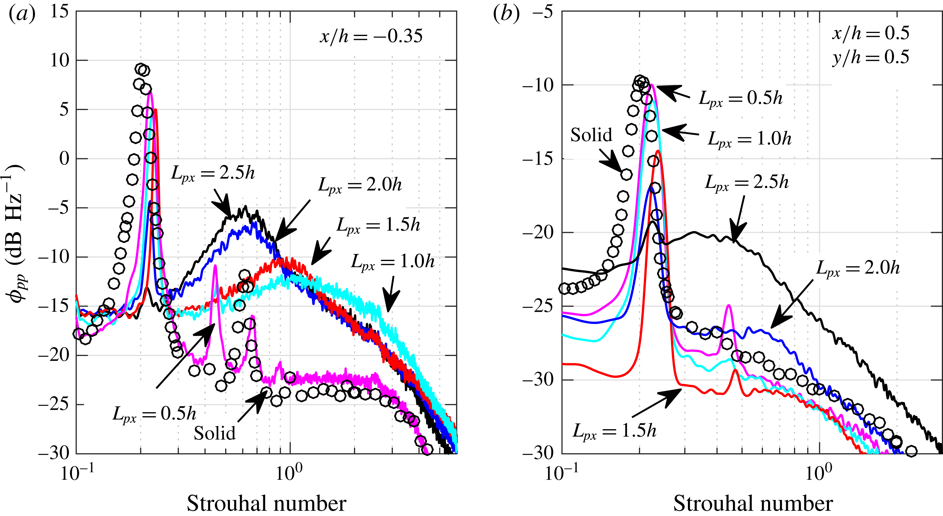
Time history of the surface pressure collected by transducers
 $p1$
at
 $x/h=-0.35$
for solid, 80 PPI and 25 PPI porous treatments.

Power spectral density of pressure measured by transducers
 $p6$
at
 $x/h=-1.9$
(a),
 $p4$
at
 $x/h=-1.3$
(b),
 $p2$
at
 $x/h=-0.7$
(c),
 $p1$
at
 $x/h=-0.35$
(d). Solid trailing edge (——), porous 80 PPI trailing edge (——), porous 25 PPI trailing edge (- - -), background noise (
 $\cdots \cdots$
), Goody model (●).

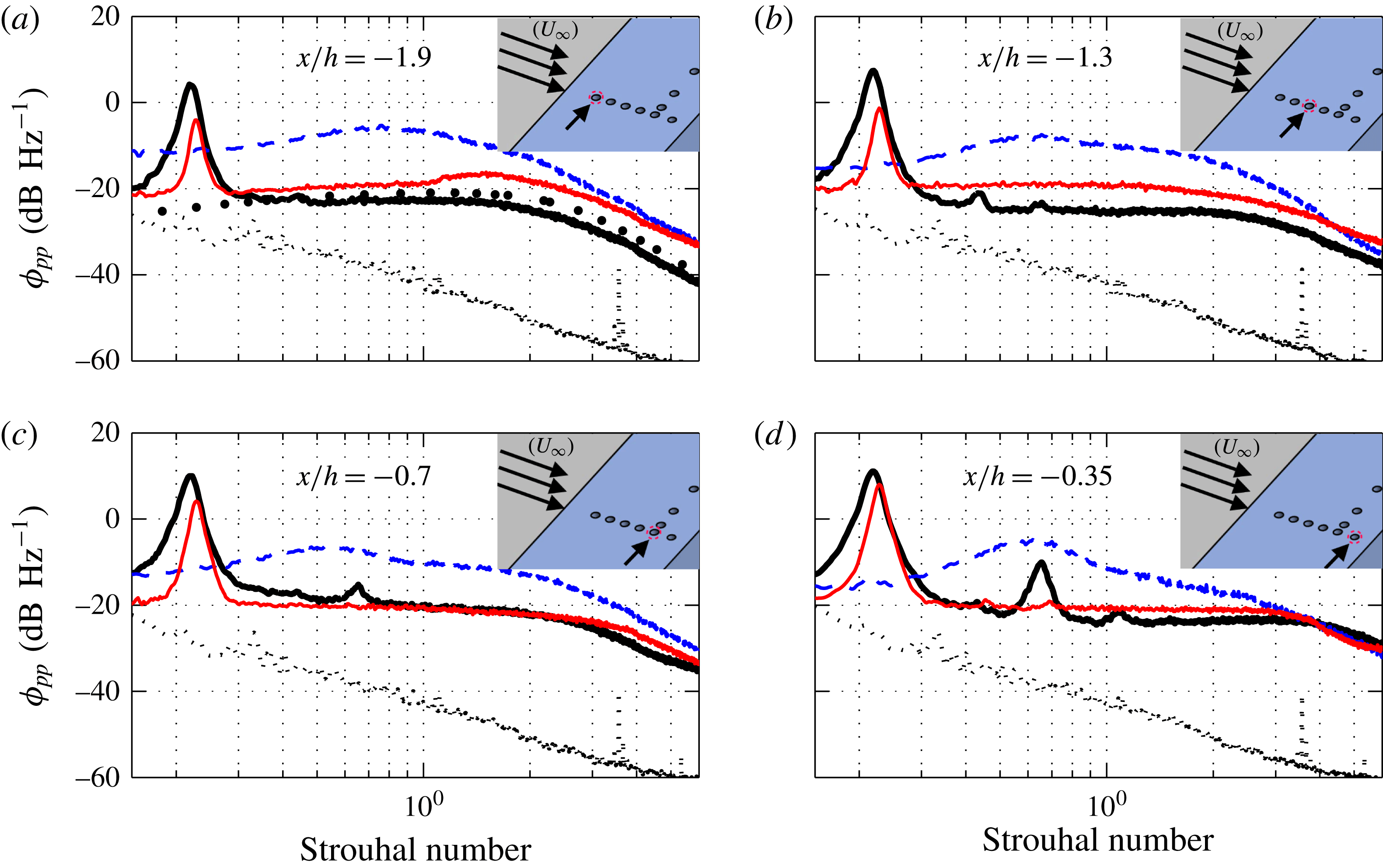
The power spectral density of the surface pressure fluctuations (
 $\unicode[STIX]{x1D719}_{pp}$
) obtained from the pressure transducers
 $p1$
,
 $p2$
,
 $p4$
and
 $p6$
are presented in figure 13. To demonstrate the validity of the data, the single-point wall pressure spectrum for the solid trailing-edge case at
 $x/h=-1.9$
, where the effects of the pressure gradient are minimum, is compared against the Goody model (Goody Reference Goody2004). The results from Goody’s model have been corrected for presentation in figure 13 by taking into account the inner layer information of the boundary layer. The comparison shows an overall good agreement, particularly for the broadband aspect of the spectra with a slope of
 $\unicode[STIX]{x1D714}^{-0.7}$
at low frequencies and
 $\unicode[STIX]{x1D714}^{-0.5}$
at higher frequencies, as shown in Goody (Reference Goody2004). The results, however, show minor deviations at low frequencies, where the vortex shedding tonal peak is observed and about
 $\pm$
1.7 dB at the middle and high frequency regions. The vortex shedding peak can be seen at
 $St\approx 0.21$
at all transducer locations for the solid case with the peak for the porous 80 PPI slightly shifted to higher
 $St$
numbers. Similar to the results obtained in figure 10, no tonal peak is seen for the case of porous 25 PPI, which again confirms that the vortex shedding has been effectively attenuated using the porous treatment in the near-wake region. The tonal peak for the case of solid trailing edge protrudes by about 10 dB above the broadband energy content while that for porous 80 PPI is of the order of 8 dB, and almost negligible for porous 25 PPI for the transducer located at the trailing edge (
 $x/h=-0.35$
). Results have also shown that the porous treatment can increase the broadband energy content in the whole frequency range due to (i) the frictional forces between the flow and the rough porous surface and (ii) the hypothesized hydrodynamic field inside the porous medium. The comparison of the surface pressure fluctuations results for the 25 PPI surface and the velocity PSD results near the wall (figure 10(
 $BP_{1{-}3},BL_{4}$
)) and in the near wake (figure 11) show the development of a similar broadband hump at approximately
 $St\approx 0.5$
.
3.5 On the source of the broadband hump
As discussed above, the rise in the surface pressure fluctuations and the velocity energy level near the surface in the case of porous trailing edges is believed to be partly due to the frictional forces acting on the rough surface of the porous materials (figure 6). However, the roughness alone does not seem to be the sole reason for the existence of a distinct broadband hump at approximately
 $St\approx 0.5$
, which also only appears for the 25 PPI material and dissipates rapidly with distance. As hypothesized earlier, the broadband hump can also be due to a hydrodynamic field inside the porous medium. In order to only focus on the frictional forces and eliminate the possibility of the emergence of any hydrodynamic field inside the porous medium, the porous medium was filled with very fine grain sand. By filling the porous section with sand, at different heights (
 $h_{s}$
), as shown in figure 14, the effect of surface roughness and the internal hydrodynamic field can be examined independently.
Power spectral density of pressure measured by transducers
 $p4$
at
 $x/h=-1.3$
(a) and
 $p2$
at
 $x/h=-0.7$
(b), with different thickness of porous 25 PPI trailing edge filled with sand. Solid trailing edge (circle line); 100 % sand (——); 90 % Sand (-
 $\cdot$
-
 $\cdot$
); 75 % sand (
 $\cdots \cdots$
); 50 % sand (- - -); 0 % sand (——).

The effects of porous surface roughness has been examined by filling the porous 25 PPI trailing edge with different sand heights (
 $h_{s}$
), namely 0 %, 50 % (10 mm), 75 % (15 mm), 90 % (18 mm) and 100 % (20 mm) filled, relative to the porous section thickness (
 $h=20~\text{mm}$
), as shown in figure 14. Therefore, the
 $h_{s}/h=0$
and
 $h_{s}/h=1.0$
cases correspond to, respectively, a fully permeable and fully blocked (i.e. no internal hydrodynamic field but with rough surface) porous sections. In order to ensure there is no leakage of flow through the sand–porous medium and also to avoid sand leaving the porous section during the wind tests, the sand was slightly dampened. The surface pressure PSD results are presented for two locations
 $x/h=-1.3$
(
 $p4$
) and
 $-0.7$
(
 $p2$
) upstream of the trailing edge. The comparison of the fully filled porous section
 $h_{s}/h=1.0$
with the solid trailing-edge case shows that the surface roughness can generally increase the broadband content of the surface pressure fluctuations over the entire frequency range. This confirms that two different mechanisms are responsible for the increase in the surface pressure PSD and that the broadband hump at around
 $St\approx 0.5$
is not due to the surface scrubbing effects. The emergence of the broadband hump at
 $St\approx 0.5$
can only be seen for the configurations with fully permeable (0 % sand) or slightly filled (50 % sand) cases. It can also be observed that the broadband hump gradually disappears as the sand level in the porous section increases, i.e. no space left for the emergence of a strong hydrodynamic field. Also, results in figure 14 clearly show that the fundamental vortex shedding tone at
 $St=0.21$
disappears only for the partially filled porous cases with
 $h_{s}/h<0.5$
. Hence, it is anticipated that the emergence of the broadband hump in the case of highly permeable porous media (25 PPI) is related to the emergence of a flow recirculation zone inside the porous section. To further deepen our understanding of the nature of this flow recirculation zone and its importance for flow control purposes, further pressure–velocity correlation and coherence analysis have been carried out, which will be presented in § 4.
4 Flow velocity and pressure correlation analysis
The results in § 3 showed that the implementation of a porous trailing edge can lead to effective manipulation of the boundary layer, the wake flow field and the possibility of elimination of flow recirculation and vortex shedding. The results of the surface pressure and velocity fluctuations also demonstrated that the energy content of the boundary layer and wake turbulence structures can be effectively reduced. In this section, we will further investigate the changes to the boundary layer flow structures by studying the correlation and coherence of the surface pressure and velocity signals over the solid and porous surfaces. These results will enable us to better understand the underlying physics of the flow–porous surface interaction and the mechanisms leading to the stabilization of the flow over the blunt trailing edge and elimination of vortex shedding.
4.1 Surface pressure lateral coherence and length scale
The interaction of the flow with porous medium will not only change the boundary layer and wake flow velocity profiles, but also the coherence of the turbulent structures in the flow. To understand these effects, we shall study the spanwise coherence of the turbulent structures and their corresponding length scale using the pressure transducers (
 $p2$
,
 $p7$
–
 $p11$
), distributed along the span at
 $x/h=-0.7$
. The coherence between the spanwise transducers and the lateral length scale can be found from (4.1) and (4.2), respectively,
 $$\begin{eqnarray}\unicode[STIX]{x1D6FE}_{p_{i}^{\prime }p_{j}^{\prime }}^{2}(f,\unicode[STIX]{x1D709}_{z})=\frac{|\unicode[STIX]{x1D6F7}(f,p_{i}^{\prime },p_{j}^{\prime })|^{2}}{|\unicode[STIX]{x1D6F7}(f,p_{i}^{\prime },p_{i}^{\prime })||\unicode[STIX]{x1D6F7}(f,p_{j}^{\prime },p_{j}^{\prime })|},\end{eqnarray}$$
and
 $$\begin{eqnarray}\unicode[STIX]{x1D6EC}_{p,3}(f)=\int _{0}^{\infty }\unicode[STIX]{x1D6FE}_{p_{i}^{\prime }p_{j}^{\prime }}(f,\unicode[STIX]{x1D709}_{z})\,\text{d}\unicode[STIX]{x1D709}_{z},\end{eqnarray}$$
where
 $\unicode[STIX]{x1D6F7}(f,p_{i}^{\prime },p_{j}^{\prime })$
denotes the cross-power spectral density between two pressure signals, and
 $\unicode[STIX]{x1D709}_{z}$
is the separation distance between the pressure transducers in the
 $z$
-direction.
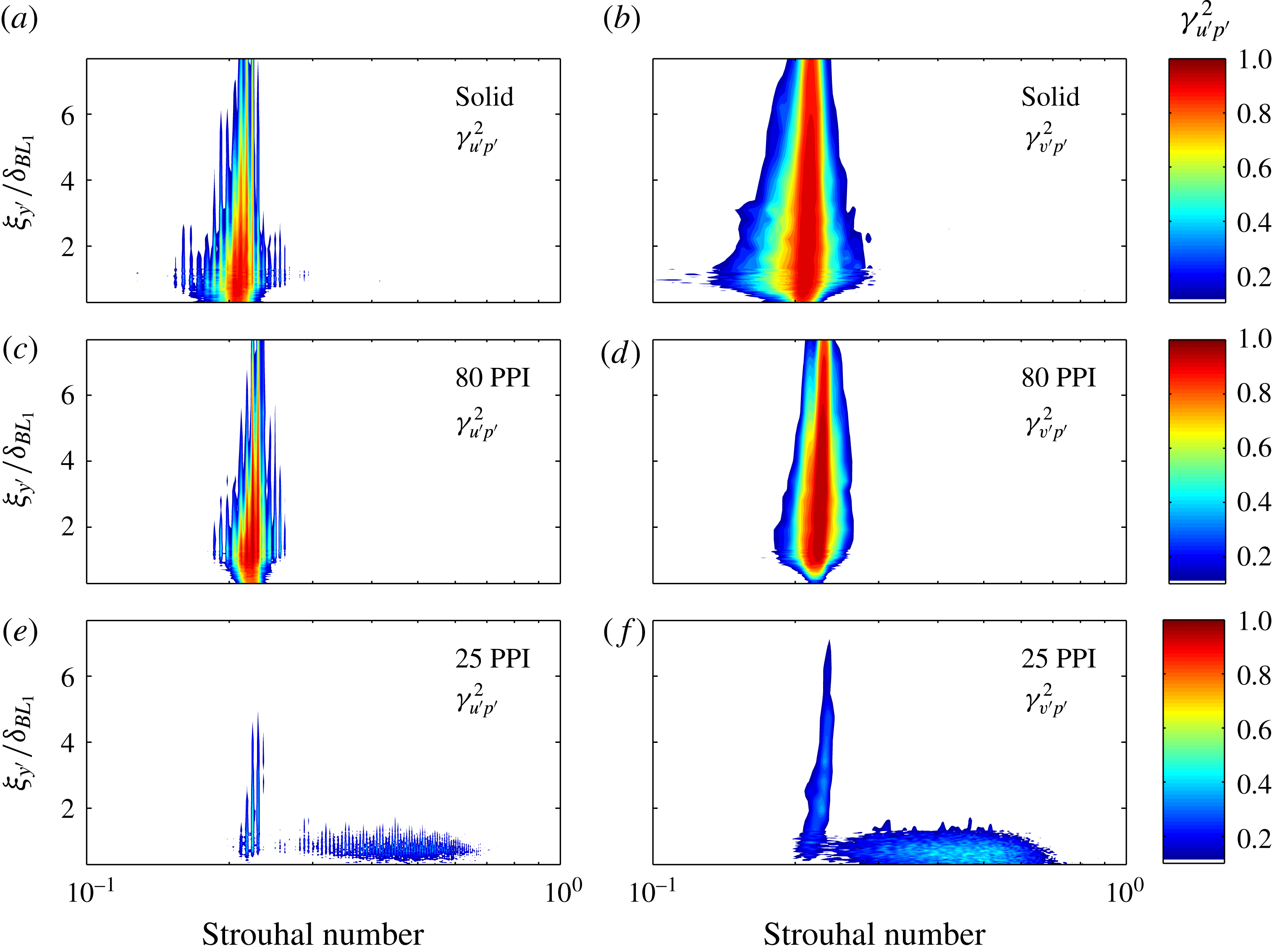
Figure 15 presents the lateral coherence measured between the spanwise transducers at
 $x/h=-0.7$
for a wide range of lateral spacings
 $0<\unicode[STIX]{x1D709}_{z}/h<4$
. The left column plots (a,c,e) show the coherence for five spanwise distances between the selected transducers while the right column plots (b,d,f) show the coherence contour plots for all 15 combinations of the spanwise distances between the six transducers. The coherence (
 $\unicode[STIX]{x1D6FE}_{p_{i}^{\prime }p_{j}^{\prime }}^{2}$
) results are plotted as a function of the Strouhal number (
 $fh/U_{\infty }$
). In the case of the solid trailing edge, as expected, a strong coherence can be observed at the vortex shedding frequency,
 $St\approx 0.21$
between the pressure signals. The results clearly show that different porous treatments have a significant and distinct effect on the lateral coherence of the flow structures, depending on the mechanical properties of the porous material. In the case of the porous 80 PPI trailing edge, while a strong coherence can be observed at the fundamental vortex shedding frequency
 $St\approx 0.21$
, the lateral coherence of the turbulent structure decays quickly with
 $\unicode[STIX]{x1D709}_{z}$
at other frequencies. On the contrary, the 25 PPI material exhibits much lower coherence values and eliminates the vortex shedding peak entirely. However, similar to the results in figures 10 (
 $BP_{1{-}3},BL_{4}$
), 11 and 13, an area of broadband hump emerges at around
 $St\approx 0.5$
. As discussed in §§ 3.4 and 3.5, this area is believed to be due to the emergence of a strong hydrodynamic field inside the porous medium.
Lateral coherence between spanwise transducers at
 $x/h=-0.7$
,
 $\unicode[STIX]{x1D709}_{z}/h=0.23$
(——),
 $\unicode[STIX]{x1D709}_{z}/h=0.67$
(——),
 $\unicode[STIX]{x1D709}_{z}/h=1.37$
(- - -),
 $\unicode[STIX]{x1D709}_{z}/h=2.33$
(
 $\cdots \cdots$
),
 $\unicode[STIX]{x1D709}_{z}/h=4.07$
(-
 $\cdot$
-
 $\cdot$
).

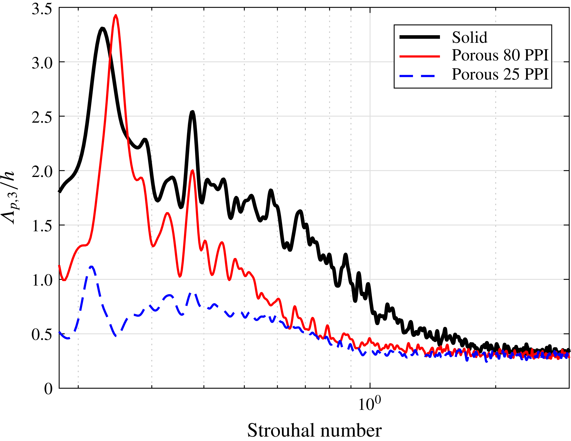
Figure 16 shows the effect of porous trailing-edge on the spanwise correlation length (
 $\unicode[STIX]{x1D6EC}_{p,3}$
) calculated using (4.2), based on the coherence of the pressure fluctuations between the spanwise transducer. In the case of the solid trailing edge, the spanwise correlation length peaks at the fundamental vortex shedding frequency (
 $St\approx 0.2$
), reaching
 $\unicode[STIX]{x1D6EC}_{p,3}\approx 3.3h$
. The results show another peak at
 $St\approx 0.4$
(
 $\unicode[STIX]{x1D6EC}_{p,3}\approx 2.5h$
), followed by a gradual decay at higher frequencies. For the porous 80 PPI case, while the results peak at
 $St\approx 0.2$
and 0.4, reaching similar values of the solid trailing edge, the correlation length at other frequencies are much lower, consistent with the results in figure 15. Finally, the results for the trailing edge fitted with porous 25 PPI show a very different behaviour. The spanwise length-scale over the entire frequency range of interest is significantly smaller (
 $\unicode[STIX]{x1D6EC}_{p,3}<h$
) than the two other cases, with no evidence of strong vortex shedding. The length scale curve in the case of the porous 25 PPI trailing edge shows a mild peak at approximately
 $St\approx 0.5$
, which is again consistent with the observations in figures 10 (
 $BP_{1{-}3},BL_{4}$
), 11 and 13.
Spanwise length scales based on the wall surface pressure measurement along the span at
 $x/h=-0.7$
.

4.2 Surface pressure temporal correlation analysis
The temporal characteristics of the boundary layer structures can be acquired from the autocorrelation of the wall pressure fluctuations, defined as,
 $$\begin{eqnarray}R_{p_{i}^{\prime }p_{i}^{\prime }}(\unicode[STIX]{x1D70F})=\frac{\overline{p_{i}^{\prime }(x_{i},t+\unicode[STIX]{x1D70F})p_{i}^{\prime }(x_{i},t)}}{p_{i_{rms}}^{\prime 2}(x_{i})},\end{eqnarray}$$
where
 $p_{i}^{\prime }$
is the wall pressure signal collected from the pressure transducer at the location
 $(x_{i},y_{i})$
,
 $p_{i_{rms}}^{\prime }$
is the root-mean-square of
 $p_{i}^{\prime }$
,
 $\unicode[STIX]{x1D70F}$
denotes the time delay between the pressure signals and the overbar represents the time averaging.
Figure 17 shows the autocorrelations of the surface pressure fluctuations,
 $R_{p_{i}^{\prime }p_{i}^{\prime }}(\unicode[STIX]{x1D70F})$
, for transducers at different locations from the trailing edge, i.e.
 $x/h=-0.35$
(
 $p1$
),
 $x/h=-0.7$
(
 $p2$
),
 $x/h=-1.3$
(
 $p4$
) and
 $x/h=-1.9$
(
 $p6$
). The results are presented in terms of the normalized time delay
 $\unicode[STIX]{x1D70F}^{\ast }=\unicode[STIX]{x1D70F}U_{\infty }/h$
. The autocorrelation result of a standard zero-pressure-gradient boundary layer at
 $Re_{\unicode[STIX]{x1D703}}=4.0\times 10^{3}$
is also presented for comparison. For the solid trailing edge, the autocorrelation results show a slowly decaying periodic behaviour, indicating the existence of a strong upstream-moving hydrodynamic field due to the vortex shedding, covering the entire trailing-edge area. The peak-to-peak distance observed in the
 $R_{p_{i}^{\prime }p_{i}^{\prime }}(\unicode[STIX]{x1D70F})$
results for the solid trailing edge (
 $\unicode[STIX]{x1D70F}_{vs}^{\ast }$
) corresponds to the vortex shedding, occurring in the near-wake region.
Autocorrelation of wall pressure fluctuations as a function of
 $\unicode[STIX]{x1D70F}^{\ast }=\unicode[STIX]{x1D70F}U_{\infty }/h$
for transducers
 $(p6)$
at
 $x/h=-1.9$
(a),
 $(p4)$
at
 $x/h=-1.3$
(b),
 $(p2)$
at
 $x/h=-0.7$
(c),
 $(p1)$
at
 $x/h=-0.35$
(d). Solid trailing edge (——), porous 80 PPI trailing edge (——), porous 25 PPI trailing edge (- - -), standard boundary layer (
 $\cdots \cdots$
).

The autocorrelation curves for the porous 80 PPI trailing edge are suggestive of two simultaneous phenomena, namely an envelope of a strong periodic hydrodynamic field and a sharp decay in the correlation that occurs at about
 $\unicode[STIX]{x1D70F}^{\ast }=0$
. The periodic behaviour observed in the 80 PPI case indicates that a strong upstream-travelling hydrodynamic field due to the vortex shedding can still be observed, although its amplitude is lower than the solid trailing edge and decays faster in the upstream direction. The sharp decay observed at about
 $\unicode[STIX]{x1D70F}^{\ast }=0$
, on the other hand, is associated with the pressure exerted by the boundary layer turbulent structure at the transducer location. It can be seen that for the porous 80 PPI trailing-edge case, at the furthest upstream transducer location (figure 17
a), the strong upstream-travelling periodic hydrodynamic field has, to a large extent, been eliminated and the autocorrelation is reduced to that of a short-lived downstream-travelling boundary layer related fluctuations.
Finally, the autocorrelation results for the porous 25 PPI trailing edge seem to indicate the existence of two concurring mechanisms, a quasi-periodic hydrodynamic field with the periodicity of
 $\unicode[STIX]{x1D70F}_{hf}^{\ast }$
and a fast-decaying event at around
 $\unicode[STIX]{x1D70F}^{\ast }=0$
. As observed in figure 17(d) for the transducer near the trailing edge (
 $p1$
), the autocorrelation experiences a fast decay at
 $\unicode[STIX]{x1D70F}^{\ast }=0$
, which is due to pressure signature of the downstream-moving boundary layer structures, similar to a standard boundary layer. The autocorrelation results within
 $1<|\unicode[STIX]{x1D70F}^{\ast }|<3$
also shows a periodic behaviour, whose periodicity corresponds to the hump frequency previously observed in figure 13 for the surface pressure fluctuations. This quasi-periodic structure, as discussed in figure 14, is believed to be due to the internal hydrodynamic field within the porous medium. Moving further upstream to
 $x/h=-1.3$
(
 $p4$
) and
 $x/h=-1.9$
(
 $p6$
), one can observe that the autocorrelation results and the hydrodynamic field decays much faster over a smaller region of
 $\unicode[STIX]{x1D70F}^{\ast }$
, similar to that of a standard boundary layer, which again corresponds to the pressure exerted by the boundary layer structures travelling over the transducers. The results also show that the fast-decaying (spatially and temporally) quasi-periodic hydrodynamic field in the case of highly permeable porous media can only be observed within a certain distance from the trailing edge (approximately
 $L_{px}=h$
). The critical porous section length required to enable flow penetration and generation of the internal hydrodynamic field will be discussed in § 5.
4.3 Boundary layer velocity–pressure coherence analysis
Figure 18 shows the coherence between the velocity and surface pressure signals at
 $p1$
, (
 $x/h=-0.35$
), corresponding to the main region where strong flow acceleration occurs (see figures 4 and 6). The coherence between the velocity and surface pressure signals is defined as,
 $$\begin{eqnarray}\unicode[STIX]{x1D6FE}_{u_{i}^{\prime }p_{i}^{\prime }}^{2}(f,\unicode[STIX]{x1D709}_{y^{\prime }})=\frac{|\unicode[STIX]{x1D6F7}(f,u_{i}^{\prime },p_{i}^{\prime })|^{2}}{|\unicode[STIX]{x1D6F7}(f,u_{i}^{\prime },u_{i}^{\prime })||\unicode[STIX]{x1D6F7}(f,p_{i}^{\prime },p_{i}^{\prime })|},\end{eqnarray}$$
where
 $\unicode[STIX]{x1D6F7}(f,p_{1},u_{2})$
denotes the cross-power spectral density function between the velocity and pressure signals. The left and right columns in figure 18 show the coherence of the
 $u$
- and
 $v$
-components of the flow velocity with the pressure signal (
 $\unicode[STIX]{x1D6FE}_{u^{\prime }p^{\prime }}^{2}$
,
 $\unicode[STIX]{x1D6FE}_{v^{\prime }p^{\prime }}^{2}$
), respectively.
Velocity–pressure coherence,
 $\unicode[STIX]{x1D6FE}_{u^{\prime }p^{\prime }}^{2}$
(a) and
 $\unicode[STIX]{x1D6FE}_{v^{\prime }p^{\prime }}^{2}$
(b) at location
 $p1$
, (
 $x/h=-0.35$
) for solid, porous 80 PPI and porous 25 PPI trailing edges.

Figure 18 presents the coherence between the streamwise and vertical flow velocities and the surface pressure fluctuations measured at
 $x/h=-0.35$
for the solid and porous trailing edges. The results in figure 18 show a strong coherence at the vortex shedding frequency,
 $St\approx 0.2$
for the case of solid trailing edge. The velocity–pressure coherence becomes broader and covers a wider range of frequencies (
 $0.15\lesssim St\lesssim 0.3$
) at about the flow velocity overshoot region (
 $y^{\prime }/\unicode[STIX]{x1D6FF}_{BL_{1}}=1$
), particularly for the coherence between the vertical flow velocity component
 $\unicode[STIX]{x1D6FE}_{v^{\prime }p^{\prime }}^{2}$
. The
 $\unicode[STIX]{x1D6FE}_{v^{\prime }p^{\prime }}^{2}$
coherence results for the porous 80 PPI trailing edge show a similar strong coherence at the vortex shedding frequency,
 $St\approx 0.2$
, but with a narrower coherence width (
 $0.2\lesssim St\lesssim 0.25$
) at
 $\unicode[STIX]{x1D709}_{y^{\prime }}/\unicode[STIX]{x1D6FF}_{BL_{1}}=1$
, which indicates the reduction of the flow acceleration over the trailing edge. In contrast, a much weaker coherence can be seen at the vortex shedding frequency for the case of the porous 25 PPI trailing edge, which is consistent with the small peaks observed in figure 13(
 $x/h=-0.35$
). Note that, this spectral peak for the case of the 25 PPI material is not visible in the near-wall velocity spectra results (figure 10
i). However, at the locations farther from the surface (figure 10
g) and in the near wake (figure 11 (
 $x/h=0.1$
)), the peaks become slightly more visible but strongly attenuated. These findings prove that the energy field due to vortex shedding for the porous 25 PPI trailing edge is weak, which also corresponds to the delayed vortical structures from the trailing edge, as seen in figure 4. It can be seen that a relatively large area of high velocity–pressure coherence broadband region emerges between
 $St=0.3$
and
 $St=0.9$
and
 $0\lesssim \unicode[STIX]{x1D709}_{y^{\prime }}/\unicode[STIX]{x1D6FF}_{BL_{1}}\lesssim 2$
, similar to the results obtained in the boundary layer velocity spectra profiles presented in 10(a,d,g) and 13. Unlike the behaviour observed for the energy field from vortex shedding, this broadband region is confined within a spatial domain and dissipates quickly with
 $x$
and
 $y$
. This again confirms that this is due to a localized flow circulation hydrodynamic field inside the porous medium, which only occurs in the case of porous materials with high permeability. As shown earlier in figure 17, the emergence of this hydrodynamic field requires a long enough porous section for enabling flow–porous interaction and flow penetration into the porous medium. In the next section, we will examine the effects of the porous section length on the emergence of the internal hydrodynamic field and control of the flow.
5 Flow penetration critical length
The results in § 3 have demonstrated that the use of a highly permeable trailing-edge section for a blunt flat plate can lead to the reduction of flow acceleration at the trailing edge, delay of flow recirculation, attenuation of vortex shedding and reduction of the energy–frequency content of the turbulence structures within the boundary layer and wake. The velocity–pressure coherence analysis in § 4, on the other hand, showed that a quasi-period hydrodynamic field may emerge within the porous medium. It has also become clear from the results in the previous sections that the boundary layer flow penetration into the porous medium and then discharges into the near-wake region plays an important role in the above-mentioned effects. To enable a proper flow penetration, the flow requires to remain in contact with the porous section over a long enough surface. The results presented in the previous sections had been obtained for porous sections with a streamwise length of
 $L_{px}=2.5h$
. In order to find out the critical length required to achieve effective flow control, further experiments have been carried out for porous trailing edges (25 PPI) with different lengths, i.e.
 $L_{px}/h=0.5,1.0,1.5,2.0$
and
 $2.5$
.
Figure 19 compares the time-averaged normalized streamwise velocity (
 $U$
) around the trailing edge of the flat plate fitted with different lengths of porous material. The solid trailing-edge result is also provided for comparison. The results in figure 19 show that the flow recirculation after the porous trailing edge shrinks with
 $L_{px}$
and detaches from the trailing-edge surface for
 $L_{px}>1$
. The results also reveal that the amount of flow discharge from the whole length of the blunt trailing edge over
 $-0.5<y<0.5$
increases with
 $L_{px}$
. One can, therefore, link the axial shift in the flow recirculation to the amount of flow discharge from the porous medium, which itself depends on the porous surface length and boundary layer flow penetration into the porous medium. Another interesting observation is the effect of the porous section length on the flow acceleration zone above the trailing edge. It can be observed that in the case of long enough porous sections, the uniform flow discharge from the blunt trailing-edge reduces the velocity gradient in the vertical direction and weakens the flow acceleration.
Time-averaged streamline flow pattern with different porous section lengths (
 $L_{px}$
).

(a) Wall pressure fluctuations with different porous 25 PPI trailing-edge lengths at
 $x/h=-0.35$
 $(p1)$
. (b) The power spectral density of the streamwise velocity in the wake at
 $x/h=0.5$
and
 $y/h=0.5$
.

The effect of the porous section length can be further analysed using the wall pressure power spectral density results (
 $\unicode[STIX]{x1D719}_{pp}$
) at a point near the trailing edge,
 $x/h=-0.35$
 $(p1)$
, as presented in figure 20(a). Results are presented for five porous section lengths (
 $L_{px}/h=2.5,2,1.5,1$
and
 $0.5$
) and also the solid trailing edge. The localized broadband hump observed previously in the surface pressure results (figure 13) is shown to be highly sensitive to the porous section length. It can be seen apparently that the broadband hump appears only for the long porous treatments. Results also show that the fundamental vortex shedding frequency at
 $St=0.21$
become stronger and approaches that of a solid trailing edge for the shorter porous treatments. This shows that the shorter porous treatments do not have a particularly strong internal hydrodynamic field and are also unable to attenuate the vortex shedding. The influence of the porous trailing-edge treatment length on the flow recirculation in the near-wake region was also investigated in this study. Figure 20(b) shows the wake flow velocity PSD (
 $\unicode[STIX]{x1D719}_{uu}$
) at
 $x/h=0.5$
and
 $y/h=0.5$
obtained using a single hot-wire probe. The results evidently show that the use of shorter porous sections (
 $L_{px}=1.5h,1h$
and
 $0.5h$
) can barely change the tonal behaviour of the flow at the fundamental (
 $St=0.21$
) and the first harmonic (
 $St=0.45$
) frequencies. The results show that the suppression of the tonal peaks and the emergence of the broadband hump occurs only for the porous section lengths of
 $L_{px}=2.5h$
and
 $2h$
. This confirms that the attenuation of the near-wake vortex shedding can be attributed to the emergence of a quasi-periodic flow recirculation field inside the porous medium.
Finally, to better understand the emergence of the internal hydrodynamic field and its relationship with the porous treatment length (
 $L_{px}$
), detailed pressure autocorrelation and velocity–pressure coherence studies have been carried out. Figure 21 summarizes the autocorrelation and the velocity–pressure coherence (
 $\unicode[STIX]{x1D6FE}_{u^{\prime }p^{\prime }}^{2}$
) results for the
 $p1$
transducer (
 $x/h=-0.35$
), where flow acceleration is expected. Results are presented for different porous treatment lengths. The surface pressure autocorrelation result for a standard zero-pressure-gradient boundary layer at
 $Re_{\unicode[STIX]{x1D703}}=4.0\times 10^{3}$
(dotted-line) and the solid trailing edge (circles) are also provided for the sake of comparison. As expected, the autocorrelation for a standard boundary layer decays quickly to nearly zero within
 $1<|\unicode[STIX]{x1D70F}^{\ast }|<3$
, while in the case of the solid trailing edge
 $R_{p_{i}^{\prime }p_{i}^{\prime }}$
has a strong periodic behaviour, due to the vortex shedding, and maintains its amplitude for a long period of time (
 $\unicode[STIX]{x1D70F}^{\ast }$
). The autocorrelation results for the porous trailing edges confirm again that there exists a critical length for the elimination of the vortex shedding and the emergence of the quasi-periodic hydrodynamic field within the porous medium. The quasi-periodic internal hydrodynamic field for the long porous treatments, particularly for the cases with
 $L_{px}>1.5h$
, manifests itself as a fast-decaying oscillation within
 $1<|\unicode[STIX]{x1D70F}^{\ast }|<3$
in the pressure autocorrelation results and as a broadband high coherence region near the wall in the pressure–velocity coherence figures. The velocity–pressure coherence results also confirm the attenuation of vortex shedding and emergence of a broadband hump for the long porous treatments. Finally, one can conclude based on the pressure and velocity PSD and coherence results that (i) the suppression of flow acceleration and the delay of flow recirculation depends on the level of flow discharged from the porous medium into the wake, (ii) to ensure enough flow discharge into the near-wake region, a relatively long porous section of about
 $L_{px}=2h$
is required, (iii) the use of a relatively long porous section can lead to the emergence of a quasi-periodic flow recirculation region in the porous section, which then results in a localized fast-decaying broadband hump.
Autocorrelation of the wall pressure fluctuations with different porous 25 PPI trailing-edge lengths at
 $x/h=-0.35$
 $(p1)$
. Solid trailing edge (circle line);
 $L_{px}=2.5h$
(——);
 $L_{px}=2.0h$
(- - -);
 $L_{px}=1.5h$
(-
 $\cdot$
-
 $\cdot$
);
 $L_{px}=1.0h$
(——, green);
 $L_{px}=0.5h$
(——, black), standard boundary layer (
 $\cdots \cdots$
).

6 Concluding remarks
The use of porous materials for aerodynamic and aeroacoustic purposes has been the subject of many numerical investigations in the past. This paper is an experimental attempt to shed some light on the underlying physics of some of the phenomena observed previously in other studies and provide an evidence-based discussion on other potential candidates responsible for flow and noise control using porous media. To do so, a simple flat plate with blunt trailing edge was used to study the effects of using porous treatments at the trailing edge for controlling the flow acceleration and vortex shedding. While the experimental set-up is relatively simple, it provides a good platform for investigating various issues concerning flow–porous interaction, such as flow scrubbing, flow penetration, flow acceleration, vortex shedding and noise generation. Results have shown that the flow penetration into the porous trailing-edge section and then discharge into the near wake can lead to some complex phenomena, such as the reduction of flow acceleration over the trailing edge, delay and weakening of the vortex shedding and break-up of large coherent wake structures. The boundary layer results have also revealed that the energy content of the large low frequency boundary layer structures can be significantly reduced using a highly permeable surface. The spanwise coherence of the structures has also been shown to reduce considerably, which shows the break-up of these coherent structures. While using permeable surfaces leads to the suppression of the fundamental vortex shedding tonal frequency (
 $St=0.2$
), the emergence of a broadband hump at higher frequencies (
 $St=0.5$
) indicated the presence of a weak recirculating flow zone inside the porous medium. Results have shown that the emergence of the internal hydrodynamic field and attenuation of the vortex shedding in the near wake are related and that both depend on the length of the flow porous section interacting with the flow. Based on the experimental observation, a long enough porous section is needed to enable flow penetration into the porous medium and discharge into the wake. The results in this paper provide the impetus for further experimental and numerical studies on the use of porous treatments and development of tailored porous materials for aerodynamic and aeroacoustic applications. Also, given the complexity of the flow–porous interaction problems, as demonstrated in this study, further high-fidelity numerical studies with realistic micro-to-macro-scale modelling, can provide more insight into the underlying physics of the phenomena observed in this work.
Acknowledgement
This project is sponsored by Embraer S.A. The second author (M.A.) would like to acknowledge the financial support of the Royal Academy of Engineering.