





Non-technical Summary
Fossils from the Mascall Formation in eastern Oregon give us a window into what the Pacific Northwest looked like approximately 16 million years ago, during a time of global climate change. However, the exact age of these rocks and how the ancient forests that they preserve relate to broader regional patterns is not well known. For example, were these dense forests common across the region, or just around local lakes?
To answer this, we combined new dating of volcanic layers with plant fossils, including macrofossils, pollen, and phytoliths, using a variety of tools to reconstruct past climates and vegetation. Our findings show that this part of Oregon was covered in warm, humid, and mixed forests, and also contained warm-loving plants like palms and gingers. Occasional grassy patches likely also occurred in the region, potentially a result of disturbance. These forests were quite different from the more open grassland-like environments developing at the same time farther east, in the Rocky Mountains and Great Plains. Our results suggest that the Cascade Mountains were not yet tall enough to block moisture from the Pacific Ocean, which helped maintain these humid and forested conditions. This study shows how using multiple lines of evidence can give us a clearer picture of ancient environments and how they changed over time.
Introduction
The Pacific Northwest (PNW; USA) hosts a rich paleobotanical record providing insight into changing climate, environments, and habitats of the Cenozoic (Wolfe, Reference Wolfe1981, Reference Wolfe1994; Leopold and Denton, Reference Leopold and Denton1987). In particular, the Eocene to late Miocene sedimentary record of the John Day region of central Oregon has showcased a generalized pattern of decreasing annual temperature, increasing temperature seasonality, and decreasing precipitation through time (Meyer and Manchester, Reference Meyer and Manchester1997; Retallack, Reference Retallack1997; Dillhoff et al., Reference Dillhoff, Dillhoff, Dunn, Myers, Strömberg, O’Connor, Dorsey and Madin2009). The Mascall Formation represents the mid-Miocene component of this sequence (Fig. 1) and preserves the Mascall flora, one of several Miocene-aged floras in the PNW. Mascall fossils have long served as key biostratigraphic markers for both fauna and flora (e.g., ‘Mascall-type’ floras; Chaney and Axelrod, Reference Chaney and Axelrod1959; Wilson, Reference Wilson1960) and showcase regional terrestrial environments at the height of the Miocene Climatic Optimum (MCO), Earth’s most recent major warming event with atmospheric CO2 similar to our predicted future (Steinthorsdottir et al., Reference Steinthorsdottir, Coxall, de Boer, Huber and Barbolini2021; Hönisch et al., Reference Hönisch, Royer, Breeker, Bowen, Polissar and Ridgwell2023).
Site maps. (1) The United States overlain with modern mean annual precipitation (MAP, cm/yr) and showing major geographic and vegetation provinces and fossil plant localities the data of which are reported in this study, including the Mascall site of central Oregon. (2) State of Oregon showing discussed geographic provinces; red rectangle, see (4). (3) Generalized stratigraphic column of Oligocene–Miocene John Day region formations, including lower (L), middle (M), and upper (U) members of the Mascall Formation. (4) The John Day River valley of central Oregon (red rectangle in [2]), showing localities where macrofossil, phytolith, palynomorph, and tuff samples reported in this study were sampled. Paleobotanical localities include the Mascall type area, i.e., exposures south of the John Day River on private land. CB = Columbia Basin; EF = Eastern Forest; FCR = Fields Creek Roadcut; GP = Great Plains; M = NMR = Meadow; North Mascall Ranch; OP = Oregon Plateau; PNW = Pacific Northwest; RM = Rocky Mountains; VH = Van Horn’s Ranch; WH = White Hills.

Figure 1 Long description
Panel 1: A map of the United States colored by M A P from 0 (red) to 200 (blue) centimeters per year. Dotted lines divide the country into provinces: P N W in the Northwest, R M in the West-Central, G P in the Central, and E F in the East. White circles mark fossil localities concentrated in the P N W and R M regions.
Panel 2: A satellite map of Oregon. The Cascades run North-South in the West. C B is in the North-Central, Blue Mtns. in the Northeast, and O P in the Southeast. A red rectangle in the center-east highlights the John Day region.
Panel 3: A vertical stratigraphic column. From top to bottom: Rattlesnake Fm., Mascall Fm. (divided into U, M, and L members), Picture Gorge Basalts (Miocene), and Upper John Day Fm. (Oligocene).
Panel 4: A detailed satellite map of the John Day River valley. The John Day Fault runs East-West through the center. To the West is the Type area with N M R and other localities. To the East is the Field’s Creek area with localities M, V H, F C R, and W H. Icons indicate sample types: green leaf for Macrofossil, light green shape for Phytolith, yellow kidney shape for Palynomorph, and gray block for Dated tuff. The Aldrich Mountains are to the South and the Belshaw Fault is to the East. A scale bar indicates 5 kilometers.
Climatic changes occurring in the John Day sequence could, however, be more complex than a simple unidirectional and long-term trend. For example, late Oligocene to early Miocene paleosols from the upper John Day Formation were interpreted to indicate the presence of semiarid open habitats of grassland, shrubland, and/or woodland (Retallack, Reference Retallack1997, Reference Retallack2004; Retallack et al., Reference Retallack, Wynn and Fremd2004; Retallack and Samuels, Reference Retallack and Samuels2020), following humid forests characterizing the early Oligocene (Meyer and Manchester, Reference Meyer and Manchester1997). Kukla et al. (Reference Kukla, Rugenstein, Ibarra, Winnick, Strömberg and Chamberlain2022) tentatively likened this vegetation pattern to the roughly contemporaneous well-documented spread of open grass habitats farther inland, in the Rocky Mountains and Great Plains (Strömberg, Reference Strömberg2005; Harris et al., Reference Harris, Strömberg, Sheldon, Smith and Vilhena2017), and collectively described the changes as a broader ‘open habitat transition’ (OHT). The interpretation of an OHT in leeward environments of the southern Cascade Range, if correct, provides support for reconstructions of near-modern elevation of the range, and presence of its strong leeward rain shadow (Fig. 1), by the late Oligocene (Bershaw et al., Reference Bershaw, Cassel, Carlson, Streig and Streck2019; McLean and Bershaw, Reference McLean and Bershaw2021; Kukla et al., Reference Kukla, Rugenstein, Ibarra, Winnick, Strömberg and Chamberlain2022). However, independent paleobotanical evidence corroborating an inference of semiarid and open habitats is lacking due to a dearth of paleobotanical sites in the upper John Day Formation (Dillhoff et al., Reference Dillhoff, Dillhoff, Dunn, Myers, Strömberg, O’Connor, Dorsey and Madin2009).
In contrast to interpretations of semiarid and open habitats in the Upper John Day Formation (Retallack, Reference Retallack1997, Reference Retallack2004; Retallack et al., Reference Retallack, Wynn and Fremd2004; Retallack and Samuels, Reference Retallack and Samuels2020) and well documented in the Great Plains (Janis et al., Reference Janis, Theodor and Boisvert2002; Strömberg, Reference Strömberg2005, Reference Strömberg2011; Mihlbachler and Solounias, Reference Mihlbachler and Solounias2006), the mid-Miocene Mascall Formation generally shows evidence indicating humid climates and closed canopy habitats. For example, paleosols of the Mascall Formation lack evidence for grasslands (mollisols) or strongly seasonal precipitation (e.g., pedogenic carbonates) (Bestland et al., Reference Bestland, Forbes, Krull, Retallack and Fremd2008), and abundant paleobotanical evidence suggests the presence of mixed-deciduous, closed-canopy forests in a humid everwet climate (Gray, Reference Gray1958; Chaney and Axelrod, Reference Chaney and Axelrod1959). Early reconstructions of the Mascall flora (and the early Oligocene Bridge Creek flora) relied strongly on comparison to coastal redwood and bordering forests of northern California (Chaney, Reference Chaney1925). However, after the discovery of living Metasequoia in China in the early 1940s, the abundance of foliage and cones from the John Day region previously assigned to Sequoia were reassigned to Metasequoia and Taxodium (Chaney, Reference Chaney1951). The subsequent reinterpretation invoked mixed-deciduous humid and closed-canopy forests of the eastern USA (e.g., Louisiana swamps, and bottom lands in Indiana and Illinois) and eastern Asia (e.g., Hupeh, Szechuan) as a closest modern analog; however, no perfect modern analog for the Mascall flora exists given its association of genera that are not currently found together (Chaney and Axelrod, Reference Chaney and Axelrod1959). Thus, if semiarid climates and open to semi-open vegetation did in fact characterize the late Oligocene and early Miocene of the John Day region, climates likely reverted to more humid conditions during the mid-Miocene and a unidirectional characterization of an OHT and aridification in the PNW might not be appropriate. Alternatively, because paleobotanical evidence typically overrepresents lowland environments near water sources (Spicer, Reference Spicer1989; Greenwood, Reference Greenwood and Donovan1991), the Mascall flora could represent gallery or flood-plain forests in an otherwise more open regional vegetation type (Kukla et al., Reference Kukla, Rugenstein, Ibarra, Winnick, Strömberg and Chamberlain2022).
Although earlier paleobotanical work (e.g., 1920s–1950s) provided an indispensable foundation for the understanding of Mascall vegetation and climate, there has been limited reinvestigation. One potential reason for this is that published taxonomic justifications are often limited in scope, fossils are housed across several museums, and most are not digitized, making reinvestigation time intensive and costly. This has hindered the application of updated practices and methods to the flora. For example, earlier work largely inferred paleovegetation and paleoclimate by qualitative and species-level nearest living relative (NLR) inference (Chaney, Reference Chaney1925; Chaney and Axelrod, Reference Chaney and Axelrod1959). This approach involves morphologically matching fossil species to a living species, from which an analogous ecological and climatic preference is inferred. The reliability of using leaves to define taxonomic relatedness, and thus ecological relatedness assuming niche conservatism, at a species level across 107 yr is questionable (e.g., Wilf, Reference Wilf2008) and ignores the diversity of ecologies present within a genus. In contrast, quantitative NLR inferences drawn at the genus level are more inclusive and better represent uncertainty in subsequent ecological and climatic interpretations (e.g., Greenwood et al., Reference Greenwood, Archibald, Mathewes and Moss2005; Reichgelt et al., Reference Reichgelt, Baumgartner, Feng and Willard2023). In addition, fossil palynomorphs (pollen and spores) and phytoliths (microscopic biosilica bodies) offer critical evidence for regional-scale reconstructions of vegetation structure (Leopold et al., Reference Leopold, Liu, Clay-Poole, Prothero and Berggren1992; Strömberg et al., Reference Strömberg, Dunn, Crifò, Harris, Croft, Su and Simpson2018), with phytoliths being a key point of evidence for the OHT in the Rocky Mountains and Great Plains (Strömberg, Reference Strömberg2005; Harris et al., Reference Harris, Strömberg, Sheldon, Smith and Vilhena2017). However, published records of pollen from the Mascall Formation are limited and those of phytoliths are entirely lacking.
Advances in radioisotopic dating over the last 60 yr have yielded increasingly precise and accurate age constraints for the Mascall Formation, progressing from K-Ar (Fiebelkorn et al., Reference Fiebelkorn, Walker, MacLeod, McKee and Smith1982), Ar-Ar (Swisher, Reference Swisher1992), to, most recently, U-Pb via chemical abrasion isotope dilution thermal ionization mass spectrometry (CA-ID-TIMS) (McLaughlin et al., Reference McLaughlin, Hopkins and Schmitz2016; Maguire et al., Reference Maguire, Samuels and Schmitz2018). Similarly, recent refinements in the application of Bayesian age-depth modeling to deep-time scenarios have allowed constrained ages to be reconstructed for horizons of interest between dated tuffs (e.g., Trayler et al., Reference Trayler, Schmitz, Cuitiño, Kohn, Bargo, Kay, Strömberg and Vizcaíno2020). Such age-depth models have not yet been applied to the Mascall Formation despite the presence of several reliably dated tuffs sampled in, or near, the type area. Additionally, the primary fossil plant localities occur in the Fields Creek area, ~25 km east of the type area (Fig. 1) where no prior radioisotopic constraints exist and direct lithostratigraphic correlation to the type area is lacking. Thus, age constraints for the Mascall flora are currently imprecise.
This study reinvestigates the age, vegetation, and climate of the Mascall flora using a suite of fossil plant types (i.e., macrofossils, phytoliths, palynomorphs), providing a local to regional perspective. In addition, we increase the accessibility and reproducibility of the Mascall macrofloral record by providing plant macrofossil morphotypes details and images (Supplemental 1). Specifically we address the following research questions: (1) what is the age of the Mascall Formation and the flora therein?; (2) what type of vegetation and climate characterized the region?; and (3) is the Mascall paleobotanical record insensitive to regional hydroclimate due to a wet lowlands bias? A refined understanding of Mascall Formation paleoenvironments provides a critical perspective for assessing the timing of uplift of the Cascades, the evolution of their leeward landscape, and the habitat of the Mascall fauna. These insights might also inform more generally how ecosystems function in a warm and high CO2 world like our near future.
Geologic background
The John Day region features a fairly continuous Eocene to late Miocene record of terrestrial sedimentation (Fremd et al., Reference Fremd, Bestland and Retallack1994; Dillhoff et al., Reference Dillhoff, Dillhoff, Dunn, Myers, Strömberg, O’Connor, Dorsey and Madin2009). The mid-Miocene is represented by the Picture Gorge Basalts (PGB) and the overlying Mascall Formation. Both formations occur in the Blue Mountain province, separating the Columbia Basin to the north and the Oregon Plateau to the south (Fig. 1). The Blue Mountains themselves are a highly deformed anticlinorium involving a diverse suite of volcanic and sedimentary rocks (Walker, Reference Walker and Walker1990; Reidel et al., Reference Reidel, Camp, Tolan, Kauffman, Garwood, Reidel, Camp, Ross, Wolff, Martin, Tolan and Wells2013b) and their uplift history likely varied across the range. For example, a paleotopographic high at their south-southeastern front impeded the flow of the Imnaha basalts at 16.6 Ma (Reidel et al., Reference Reidel, Camp, Tolan, Martin, Reidel, Camp, Ross, Wolff, Martin, Tolan and Wells2013a; Kasbohm et al., Reference Kasbohm, Schoene, Mark, Murray, Reidel, Szymanowski, Barfod and Barry2023) and a high northwestern front localized deposition between the eastern and western facies of the Eocene to Oligocene John Day Formation (Robinson et al., Reference Robinson, Brem and Mckee1984) and might have influenced local gradients of precipitation (Kukla et al., Reference Kukla, Ibarra, Rugenstein, Gooley, Mullins, Kramer, Moragne and Chamberlain2021). Yet, uplift in its eastern portions, including the Wallowa Mountains, mostly postdated the CRB eruptions (Reidel and Tolan, Reference Reidel, Tolan, Reidel, Camp, Ross, Wolff, Martin, Tolan and Wells2013; Schoettle‐Greene et al., Reference Schoettle‐Greene, Duvall and Crowley2022).
In the John Day Valley, the PGBs and Mascall Formation sediments accumulated in an east-west striking structural syncline, a companion to the Aldrich Mountain anticline immediately south. The John Day fault, a steep reverse fault, runs along this east-west troughline (Fig. 1; Thayer and Brown, Reference Thayer and Brown1966). The fault and its associated subsidiary faults explain the lateral juxtaposition of near-horizontal and steeply dipping diatomaceous beds exposed in the Fields Creek roadcut, and displacement of the Picture Gorge Basalts above the Mascall Formation at the White Hills locality (i.e., the Belshaw fault; Fig. 1) (Thayer and Brown, Reference Thayer and Brown1966; Thayer, Reference Thayer1977; Kuiper, Reference Kuiper1988).
The PGBs, a formation of the Columbia River Basalt (CRB) Group, erupted at ~17–16 Ma from the Monument dike swarm and both the PGBs and its feeder dikes have a relatively restricted occurrence mainly in the Blue Mountains (Reidel et al., Reference Reidel, Camp, Tolan, Martin, Reidel, Camp, Ross, Wolff, Martin, Tolan and Wells2013a; Cahoon et al., Reference Cahoon, Streck and Koppers2023). The Mascall Formation immediately overlies the PGBs (Fig. 1) with widespread occurrence along U.S. Highway 26, west of John Day in Grant County, although it is covered over much of its extent. The formation is best exposed in its type area, southwest of the Picture Gorge (Fig. 1), and is divided into lower, middle, and upper members (Bestland et al., Reference Bestland, Forbes, Krull, Retallack and Fremd2008). The lower member consists of marginal lacustrine diatomaceous and lignitic shales overlain by tuffaceous paleosols, thin gray tuffs, and minor sandstones (Bestland et al., Reference Bestland, Forbes, Krull, Retallack and Fremd2008). A tuff in the lower part of the Mascall Formation (presumably the lower member) was dated at 16.2 ± 1.4 Ma by K-Ar (Fiebelkorn et al., Reference Fiebelkorn, Walker, MacLeod, McKee and Smith1982), and a thin tuff ~7.5 m below the base of the Mascall tuff in the lower Mascall Formation (Unit 2 of Downs, Reference Downs1956), was dated at 15.77 ± 0.35 Ma (recalculated to 15.974 ± 0.71 Ma using modern values of neutron fluence monitor standards) by Ar-Ar (Swisher, Reference Swisher1992). A minimum of 40 m of the top of the lower member is of reversed polarity and correlates to the C5Br magnetic Chron (Prothero et al., Reference Prothero, Draus and Foss2006).
The base of the Mascall tuff unit (Unit 5 of Downs, Reference Downs1956) marks the lower/middle member contact. This tuffaceous unit is 10–15 m thick and is a generally massive, fine-grained, crystal-poor tuffaceous siltstone (Bestland et al., Reference Bestland, Forbes, Krull, Retallack and Fremd2008). The Mascall Tuff can be subdivided into a lower section of friable but more massive tuffaceous siltstone, and an upper section of yellow indurated thin stratified tuffs and stacked paleosols filled with trace fossils. The Mascall tuff unit is overlain by claystone paleosols, pedolithic conglomerates, and sandstones that make up the rest of the member (Bestland et al., Reference Bestland, Forbes, Krull, Retallack and Fremd2008). A gray tuffaceous interbed in the upper Mascall tuff was dated at 15.122 ± 0.017 Ma by CA-ID-TIMS U-Pb (Maguire et al., Reference Maguire, Samuels and Schmitz2018). The Mascall tuff represents a paleomagnetic reversal to normal polarity, correlating to C5Bn2n magnetic Chron (Prothero et al., Reference Prothero, Draus and Foss2006), with the C5Br-C5Bn2n transition dated at 15.186 Ma (Raffi et al., Reference Raffi, Wade, Pälike, Beu, Cooper, Gradstein, Ogg, Schmitz and Ogg2020). Above the Mascall tuff, the middle member spans two additional reversals, correlating to C5Bn1r and C5Bn1n magnetic Chrons (Prothero et al., Reference Prothero, Draus and Foss2006) and those reversals are dated at 15.040 and 14.870 Ma, respectively (Raffi et al., Reference Raffi, Wade, Pälike, Beu, Cooper, Gradstein, Ogg, Schmitz and Ogg2020). The upper member begins at the base of a ~2 m thick conglomerate and is overlain by clay paleosols, tuff, conglomerates, and minor sandstones (Bestland et al., Reference Bestland, Forbes, Krull, Retallack and Fremd2008). It is capped at an angular unconformity by the late Miocene Rattlesnake Formation. The Kangaroo Tuff Bed in the upper member was dated to 13.564 ± 0.018 Ma by CA-ID-TIMS U-Pb (Maguire et al., Reference Maguire, Samuels and Schmitz2018).
Silicic (mainly rhyodacitic) tuffaceous deposits throughout the Mascall Formation are thought be distally sourced, potentially erupted from either the ancestral Cascades, the McDermitt, Lake Owyhee, High Rock Caldera, and Strawberry Volcanic fields, and/or the Dinner Creek Tuff eruptive center (Smith et al., Reference Smith, Bjornstad and Fecht1989; Bestland et al., Reference Bestland, Forbes, Krull, Retallack and Fremd2008; Streck et al., Reference Streck, Ferns and McIntosh2015). There is a rarity of basalt fragments in the Mascall Formation, which could suggest that rivers traversed a low-relief landscape and reworked floodplain soils and ash with little erosion of the pre-Mascall basaltic surface (Bestland et al., Reference Bestland, Forbes, Krull, Retallack and Fremd2008). Chaney and Axelrod (Reference Chaney and Axelrod1959) suggested considerable local relief, inferred from fossil plant taxa indicating slope and upland habitats, growing on nearby volcanic slopes or adjacent uplands (e.g., ancestral Aldrich Mountains)—an uncertain interpretation strongly reliant on species-level NLR inference.
The majority of historic Mascall macrofloral collections were made at several localities in the Fields Creek area (Fig. 1), ~25 km east of the Mascall Formation type area (Chaney and Axelrod, Reference Chaney and Axelrod1959), although minor collections have also been made in the type area (Krull, Reference Krull1998). The White Hills (also called Belshaw Ranch) and Van Horn’s Ranch (also called Riverbank) localities were historically most heavily sampled, with early collection and research efforts by T.C. Condon, L. Lesquereux, J.C. Merriam, F. Knowlton, and R.W. Chaney from the 1870s to 1920s (Lesquereux, Reference Lesquereux1888; Chaney, Reference Chaney1925; Chaney and Axelrod, Reference Chaney and Axelrod1959). Discontinuous exposures and a lack of marker beds have prevented direct correlation of the type and Fields Creek areas (Chaney and Axelrod, Reference Chaney and Axelrod1959; Kuiper, Reference Kuiper1988; Bestland et al., Reference Bestland, Forbes, Krull, Retallack and Fremd2008). However, the Fields Creek area fossil localities appear to closely overlie the PGBs and are comprised largely of diatomaceous and lignitic shales, and thus are placed in the lower Mascall Formation (Bestland et al., Reference Bestland, Forbes, Krull, Retallack and Fremd2008).
Materials and methods
Field work and sampling
Field work by the authors was conducted in the 2009, 2021, and 2022 field seasons. Macrofossils and rocks sampled for pollen and phytoliths were collected from lower and middle Mascall Formation exposures in the type area (south of the John Day River), at the North Mascall Ranch locality (exposure north of the John Day River), and at several localities in the Fields Creek area including Van Horn’s Ranch, White Hills, and Fields Creek roadcut (Fig. 1; Table 1). Volcanic tuffs were sampled from Van Horn’s Ranch (but not analyzed) and White Hills in the Fields Creek area. The basal tuff at White Hills (21MF-07-T-1 lower; White Hills tuff hereafter) was analyzed for U-Pb geochronology. The sample was taken from a level 0–1 m above the exposed base of the tuff (Fig. 2). In addition, two samples were collected from the Mascall Tuff by K. Maguire (Table 1). Sample KCM081182 was collected on the northern side of U.S. Highway 26 at the Ferris Creek Mascall locality (N44.49882°, W119.55013°), from ~2 m below the yellow indurated upper section of the Mascall Tuff Bed and was analyzed for U-Pb geochronology. Sample KCM1211-120 was collected south of U.S. Highway 26 (N44.50402°, W119.61948°), from a gray, pumiceous zone that interbeds with the yellow indurated portion, ~1.5 m above the lower/upper Mascall Tuff contact. The U-Pb zircon geochronology of this sample was reported by Maguire et al. (Reference Maguire, Samuels and Schmitz2018), who obtained a weighted mean 206Pb/238U date of 15.122 ± 0.017 (0.019) [0.025] Ma (95% confidence interval; MSWD = 1.65, N = 5) from five single crystals.
Mascall Formation rock samples utilized in this study for phytolith, palynology, and U-Pb zircon analyses and their lithological and stratigraphic context, including pertinent locality numbers (Loc. #). Further detail on phytolith samples are provided in Supplementals 6 and 7. Superscripts: 1 = other UWBM locality numbers are present for separate collecting events at White Hills but are not all listed here for the sake of simplicity; 2 = there are discrepancies between locality information reported by Gray (Reference Gray1958) and that included in the UCMP locality database (accessed November 2025); we followed the information reported by Gray (Reference Gray1958).

Table 1. Long description
The table consists of seven columns: Sample, Type, Lithology, Localities, Loc. #, Member, and Reference.
* Samples O R 09-51 and O R 09-62: Phytolith type, Paleosol lithology, Type Area locality, U W B M P 4784 and P 4800, Lower Member.
* Samples O R 09-161 and O R 09-85: Phytolith type, Paleosol lithology, Type Area locality, U W B M P 4909 and P 4828, Middle Member.
* Sample 21 M F-07-S-1400: Phytolith and palynology type, Diatomaceous shale, White Hills locality, U W B M P 8853, Lower Member.
* Samples P 4123 and P 4130: Palynology type, Unknown lithology, Meadow locality, U C M P P 4123 and P 4130, Lower Member, referenced from Gray 1958.
* Samples 122, 603, and P 4215: Palynology type, Unknown lithology, Van Horn’s Ranch locality, U C M P 122, 603, and P 4215, Lower Member, referenced from Gray 1958.
* Sample 878: Palynology type, Unknown lithology, White Hills or Van Horn’s Ranch, U C M P 878, Lower Member, referenced from Gray 1958.
* Sample 21 M F-07-T-1 Lower: U-P b zircon type, Tuff lithology, White Hills locality, U W B M P 8853, Lower Member.
* Sample K C M 081182: U-P b zircon type, Tuff lithology, Ferris Creek locality, Middle Member.
* Sample K C M 1211-120: U-P b zircon type, Tuff lithology, Type Area locality, Middle Member, referenced from Maguire et al. 2018.
* Sample K C M 61023a: U-P b zircon type, Tuff lithology, Type Area locality, Upper Member, referenced from Maguire et al. 2018.
Age-depth modeling results from Bacon model for the White Hills (west hill, Unit07) locality, lower Mascall Formation, alongside our measured stratigraphic section and North American Land Mammal (Tedford et al., Reference Tedford, Albright, Barnosky, Ferrusquia-Villafranca and Hunt2004) and geomagnetic (Raffi et al., Reference Raffi, Wade, Pälike, Beu, Cooper, Gradstein, Ogg, Schmitz and Ogg2020) ages. Rank plot diagrams represent the upper and lower 95% confidence intervals for single crystal ages included in the calculation of the weighted mean 206Pb/238U age (red). Ensemble ages for horizons of interest include the section and census collection top and bottoms, and the pollen and phytolith sample reported in this study. C = coarse; Cgl = conglomerate; F = fine; M = medium; S = silt.

Figure 2 Long description
The diagram is organized into three main horizontal sections.
1. Stratigraphic Column (Left): A vertical column from 0 to 23 meters. The base consists of a thick conglomerate layer labeled White Hills tuff: Modeled as instantaneous. Above this, the section contains alternating layers of diatomite, moderately-laminated siltstone, and tuff. Key horizons are marked with dashed lines extending rightward: Section bottom at 7 meters, Lowe et al census at 11 meters (marked with a green leaf icon), Pollen and phytolith sample 2 1 M F - 0 7 - S - 1 4 0 0 at 13.5 meters, and Fossiliferous top at 22.5 meters.
2. Age-Depth Model and Rank Plots (Center): The central area plots Age in M a against the stratigraphic height.
* Rank plots: A series of 13 vertical black bars represent single crystal ages. A red horizontal line marks the weighted mean 206 P b / 238 U age of 16.131 plus or minus 0.011 M a.
* Horizons of interest: Five black data points with vertical error bars correspond to the stratigraphic markers. From top to bottom, the ages are: 16.040 plus or minus 0.106, 16.088 plus or minus 0.052, 16.103 plus or minus 0.036, 16.107 plus or minus 0.032, and 16.130 plus or minus 0.012 M a.
3. Chronological Scales (Right): Three vertical bars define the temporal context from 15.9 to 16.2 M a.
* The first bar shows North American Land Mammal Ages: Barstovian at the top and Hemingfordian at the bottom.
* The second bar shows geomagnetic polarity: C 5 B r (white) and C 5 C n dot 1 n (black).
* The third bar identifies the Miocene epoch in yellow.
In addition, a macrofossil census collection was made at White Hills for reliable inference of diversity and relative abundance by accounting for all specimens assignable to a fossil morphotype (e.g., Chaney, Reference Chaney1924; Lowe et al., Reference Lowe, Greenwood, West, Galloway, Sudermann and Reichgelt2018). The census collection was made from a 70 cm horizon, ~5 m above the White Hills tuff, in roughly the middle of the westernmost of the two white hills (Fig. 2; Appendix 1). The main collection quarry spanned 5 m laterally and a small correlative quarry was sampled 23 m lateral to it. Chaney and Axelrod (Reference Chaney and Axelrod1959) stated that collections that they analyzed came from near the top of the same hill, potentially a few meters above our collection. All newly collected samples were reposited in the Burke Museum of Natural History and Culture (UWBM) in Seattle, Washington (localities P8853 and P8860).
Geochronology
All geochronology was accomplished at the Isotope Geology Laboratory at Boise State University. Heavy minerals were separated from samples of volcanic tuff using standard density and magnetic separation techniques, and a selection of elongate, prismatic crystals with axial melt inclusions typical of rapidly grown volcanic zircon were annealed at 900°C for 60 h in preparation for chemical abrasion (Mattinson, Reference Mattinson2005). Single zircons were chemically abraded in 120 μL of 29 M hydrofluoric acid (HF) in a single aggressive step at 190°C for 12 h to eliminate the effects of radiation damage and Pb loss, prior to spiking with the ET535 mixed U-Pb isotope tracer (Condon et al., Reference Condon, Schoene, McLean, Bowring and Parrish2015; McLean et al., Reference McLean, Condon, Schoene and Bowring2015). Dissolution, chemical separations, thermal ionization mass spectrometry, data reduction, and error propagation followed the methods described by Farrell et al. (Reference Farrell, Cothren, Sundberg, Schmitz, Dehler, Landing, Karlstrom, Crossey and Hagadorn2025).
Bayesian age-depth modeling
To extend age constraints beyond dated tuffs, we used two types of Bayesian age-depth models: Bacon (Blaauw and Christen, Reference Blaauw and Christen2011) and modified BChron (Trayler et al., Reference Trayler, Schmitz, Cuitiño, Kohn, Bargo, Kay, Strömberg and Vizcaíno2020). Bayesian age-depth models simulate a variety of sediment accumulation scenarios utilizing Markov Chain Monte Carlo (MCMC) resampling to reliably constrain age uncertainty (Blaauw et al., Reference Blaauw, Christen, Bennett and Reimer2018). Bacon incorporates prior knowledge on accumulation rates, imparts some consistency in those rates through section, and is thus widely applied to lacustrine sections. We applied Bacon using the rBacon R package (Blaauw and Christen, Reference Blaauw and Christen2011) at the White Hills locality where similar lithology through the section indicates a consistent lacustrine setting. Bacon splits the stratigraphic section into a (user-defined) number of segments to which accumulation rates are applied. Rates are determined by two factors: (1) the sampling of a gamma distribution of accumulation rates, the mean and shape parameters of which are user-defined, and (2) from the accumulation rate of the segment just before it (i.e., memory). Default values for gamma distribution parameters are provided by rBacon, based on Holocene lacustrine and paludal sections across the eastern USA (Goring et al., Reference Goring, Williams, Blois, Jackson, Paciorek, Booth, Marlon, Blaauw and Christen2012). Although this region is fairly analogous to Mascall Formation paleoenvironments, we implemented a custom workflow providing a greater range of mean accumulation rates as priors to account for uncertainty in rates of sedimentation and the degree of postdepositional sediment compaction. This workflow produces an ensemble age reconstruction for horizons of interest, and ensemble duration reconstructions between horizons of interest (see Appendix 2 for further detail). The new U-Pb date of the White Hills tuff was explicitly included in the model as a likelihood constraint.
To produce an age-depth model for the entire Mascall Formation, we used the modified BChron model, which does not impart consistency in depositional rates nor use a priori accumulation rates as a model input (Haslett and Parnell, Reference Haslett and Parnell2008; Trayler et al., Reference Trayler, Schmitz, Cuitiño, Kohn, Bargo, Kay, Strömberg and Vizcaíno2020). Sediment accumulation is instead modeled as events that vary in duration and amount, such that accumulation can vary more widely through section and across MCMC iterations resulting in greater bounds of uncertainty relative to Bacon. The hyperparameters of this compound Poisson-gamma prior distribution of sediment accumulation are modulated within the MCMC chains by the age likelihoods. For this reason, Bchron is more reliably applied when lithology and depositional environments vary (Trayler et al., Reference Trayler, Schmitz, Cuitiño, Kohn, Bargo, Kay, Strömberg and Vizcaíno2020), as is the case through the Mascall Formation. For age determination likelihoods, we included previously published U-Pb ages for the Kangaroo and Mascall tuffs (Maguire et al., Reference Maguire, Samuels and Schmitz2018), the new Mascall tuff U-Pb age presented in this study, ages for geomagnetic reversals (C5Bn1r/C5Bn2n and C5Bn2n/C5Bn1r; Raffi et al., Reference Raffi, Wade, Pälike, Beu, Cooper, Gradstein, Ogg, Schmitz and Ogg2020), while representing the uncertainty in their stratigraphic location (Prothero et al., Reference Prothero, Draus and Foss2006), and the new White Hills tuff U-Pb age presented in this study, which is critical for constraining the lowest Mascall Formation. The direct correlation of the White Hills section to the type area stratigraphic column via marker beds is difficult. We integrated the White Hills tuff into the BChron model using two different scenarios for the thickness of the lower Mascall Formation: an equal thickness to the type area (100 m) and the cumulative thickness that we measured across various Fields Creek area exposures that show no obvious overlap (141.5 m). This integration provided the White Hills tuff substantial uncertainty in its stratigraphic placement within the Mascall Formation column (± 22 m), which was explicitly included in the modified BChron model (see Appendix 2 for further detail). We purposefully excluded the Ar-Ar age of Swisher (Reference Swisher1992) in the lower Mascall Formation because we found that it does meet community standards of best practices in Ar-Ar radioisotopic dating (Schaen et al., Reference Schaen, Jicha, Hodges, Vermeesch and Stelten2020).
Macrofossils
Macrofossils were photographed from pre-existing and newly made collections deposited in the Smithsonian Institution’s National Museum of Natural History (USNM), the University of California Museum of Paleontology (UCMP), the University of Oregon Museum of Natural and Cultural History (UO), and the Burke Museum of Natural History and Culture (UWBM). For many specimens, fine details of leaf architecture were imaged under a stereoscope. Both type and nontype (and often uncataloged) specimens were digitized to better represent variation and incorporate potential hidden diversity. Uncataloged specimens were assigned unique image IDs (Supplemental 1).
A morphotype framework was constructed from this digital library, using the floral list of Chaney and Axelrod (Reference Chaney and Axelrod1959) as our base. This base list was updated with more recent taxonomic publications (e.g., Manchester and Donoghue, Reference Manchester and Donoghue1995) and we reinvestigated all existing morphotype delineations and assignments of taxonomic affinity. To do so, we utilized several resources, including taxonomic studies of other Cenozoic sites in North America and beyond (e.g., Buzek, Reference Buzek1971; Edwards, Reference Edwards1983; Wolfe and Tanai, Reference Wolfe and Tanai1987; Fields, Reference Fields1996; Manchester, Reference Manchester1999), modern cleared leaf collections, herbaria, and taxonomic works of modern taxa (e.g., Meyerhoff, Reference Meyerhoff1952; Farjon, Reference Farjon1990, Reference Farjon2005). When we could not reproduce determinations made in prior work, we revised morphotype concepts. However, these revisions do not currently represent formal changes of taxonomic nomenclature. Fossil images and morphotype details, including justification of morphotype delineations and taxonomic affinity, are available online via Figshare (Supplemental 1). We hope that this digital record allows for a more accessible ‘jumping off’ point to encourage future work, e.g., continual taxonomic refinement and novel reconstructions of ecology and climate.
Lastly, we established a confidence scoring system to better represent the uncertainty inherent in many assignments of taxonomic affinity, particularly for fossil foliage. A score of high (1), medium (2), or low (3) confidence was first assigned to each macrofossil morphotype in isolation (i.e., considering the single organ at the single site). Then, the confidence was increased (score decreased by 1) if additional organs with higher confidence (i.e., pollen or reproductive organs) were present for the same taxon, or if higher confidence was given to synonymous morphotypes at other sites under recent study (Lowe, Reference Lowe2024). Confidence score adjustments were applied using R (version 4.4.2; R Core Team, 2024). Further detail on this approach was provided by Lowe (Reference Lowe2024). Macrofossil diversity, including only foliar woody nonmonocot angiosperm morphotypes, was analyzed by generating sample size-based rarefaction/extrapolation curves using the iNEXT R package (Chao et al., Reference Chao, Gotelli, Hsieh, Sander, Ma, Colwell and Ellison2014; Hsieh et al., Reference Hsieh, Ma and Chao2024).
Phytoliths
Biosilica extraction was carried out on samples from the Mascall Formation between 2009 and 2024 using the method outlined by Strömberg (Reference Strömberg2005) and later publications (see Appendix 2 for further detail). Preparation includes chemical steps to remove carbonates, clays, and organic material, and isolation of phytoliths using heavy liquid. Phytoliths were viewed under 1,000× magnification and classified using a plant functional type (PFT) scheme developed in previous work (Strömberg, Reference Strömberg2005; Strömberg et al., Reference Strömberg, Dunn, Crifò, Harris, Croft, Su and Simpson2018; Schiller et al., Reference Schiller, Lowe, Dillhoff, Fields, Riley, Taggart, Schmitz and Strömberg2024) and using the UWBM’s phytolith reference collection. The assigned PFTs included (1) PALM, (2) ZINGI (Zingiberales) (3) Other FI (other forest indicator phytoliths), (4) Grass silica short cell phytoliths (GSSCP; Poaceae), (5) AQ (wet habitat plants), (6) NDG (nondiagnostic grass), and (7) NDO (nondiagnostic other). GSSCPs group can be further divided into seven additional PFT categories, including (a) APPBO (closed-habitat grasses) (b) POOID-D (Pooideae, diagnostic), (c) POOID-ND (Pooideae, nondiagnostic), (d) PAN (Panicoideae), (e) CHLOR (Chloridoideae), (f) PACMAD General, morphotypes from either C4 or C3 members of the PACMAD clade (Panicoideae, Arundinoideae, Chloridoideae, Micrairoideae, Aristidoideae, Danthonioideae); and (g) OTHG GSSCP (Poaceae; unclear origin). Enough phytoliths were counted to reach 200 diagnostic morphotypes (categories 1–4 above) to ensure statistical robustness (Strömberg, Reference Strömberg2009). Further detail is provided in Appendix 2.
We reconstructed vegetation type (structure and overall composition) by evaluating the relative abundances of diagnostic PFTs in phytolith assemblages (e.g., Strömberg, Reference Strömberg2005; Harris et al., Reference Harris, Strömberg, Sheldon, Smith and Vilhena2017). The composition of forest indicator forms (FITOT = PALM+ZINGI+Other FI) indicates the broad representation of phytolith-producing trees and shrubs (e.g., palms vs. dicots vs. conifers), the percentage of GSSCP within diagnostic phytoliths (complement to the so-called FI-t ratio) measures the importance of grasses on the landscape and roughly assesses habitat openness (Strömberg et al., Reference Strömberg, Dunn, Crifò, Harris, Croft, Su and Simpson2018), and the composition of GSSCP assemblages documents the relative abundance of closed-habitat grasses (APPBO) and different open-habitat grasses (C3 vs. C4, cool-adapted Pooideae vs. warm-adapted PACMAD).
We compared the phytolith assemblages from the Mascall Formation to published assemblages of similar age from the northern Rocky Mountains (Strömberg, Reference Strömberg2003, Reference Strömberg2005; Harris et al., Reference Harris, Strömberg, Sheldon, Smith and Vilhena2017) and central Great Plains (Strömberg, Reference Strömberg2003, Reference Strömberg2005) by (1) testing for differences in 100–FI-t (%) (100*GSSCP/(PALM+ZINGI+OtherFI+GSSCP)) using ANOVA and (2) conducting a Principal Components Analysis (PCA) of the relative abundance of diagnostic PFTs (PALM, ZINGI, Other FI, APPBO, POOID-D, POOID-ND, PAN, PACMAD [including CHLOR]) using the princomp() function in R.
Palynology
Pollen samples were analyzed to supplement the seminal work of Gray (Reference Gray1958). Samples were thoroughly washed under deionized water, crushed to mm-size, and massed to 3 ± 0.1 g. Pollen extraction followed standard maceration procedures including treatment with HCl, HF, KOH, and acetolysis (Doher, Reference Doher1980). Residues were preserved in t-BuOH and mounted in silicone oil. A minimum of 300 identifiable, terrestrial pollen grains were identified at 400× magnification and assigned to extant taxa based on comparisons with Gray (Reference Gray1958), other relevant atlases (Moore et al., Reference Moore, Webb and Collinson1991; Kapp, Reference Kapp2000), and the Jane Gray modern reference collection at UWBM. Previous pollen count data were digitized from carbon copies of the originals of Gray (Reference Gray1958) with additions to the pollen list from Gray (in Chaney and Axelrod, Reference Chaney and Axelrod1959). Terrestrial pollen data are expressed as percentages of the terrestrial pollen sum and other palynomorphs are expressed as percentages of the sum of all palynomorphs.
Paleoclimate
Paleoclimate was reconstructed from fossil plants using two approaches: leaf physiognomy proxies and the nearest living relative proxy Bioclimatic Analysis. Leaf physiognomy builds on the assumption of unchanging leaf physiognomy-climate relationships through time, whereas nearest living relative methods assume conserved climatic tolerance within lineages through time. In both cases, only taxa known from the macrofossil record are included to minimize mixing across elevational gradients. Leaf physiognomy proxies incorporate only woody, nonmonocot angiosperms and Bioclimatic Analysis incorporates all woody terrestrial plant groups (e.g., gymnosperms). Leaf physiognomy methods used include the univariate proxies leaf margin analysis (% untoothed species vs. mean annual temperature [MAT)]) and leaf area analysis (average leaf area vs. mean annual precipitation [MAP]). In addition, multivariate proxies were used, including a modified version of Climate Leaf Analysis Multivariate Program (CLAMP) that predicts WorldCLIM based climate variables from categorical leaf traits (Yang et al., Reference Yang, Spicer, Spicer and Li2011; West et al., Reference West, Reichgelt, Reyes, Buryak, Staniszewska and Basinger2024; Reichgelt and West, Reference Reichgelt and West2025), and Digital Leaf Physiognomy (DiLP), which relates multiple continuous physiognomic measurements of leaf shape, size, and tooth characteristics to MAT and MAP (Peppe et al., Reference Peppe, Royer, Cariglino, Oliver and Newman2011). For DiLP, fossil leaves were prepared and measured following the methods described by Lowe et al. (Reference Lowe, Flynn, Butrim, Baumgartner, Royer, Peppe and Peppe2024) and data were processed and paleoclimate estimates generated using the R package dilp (Butrim et al., Reference Butrim, Lowe, Flynn, Baumgartner, Peppe and Royer2024). We used the leaf margin analysis equations reported by Wing and Greenwood (Reference Wing and Greenwood1993), with associated binomial sampling error calculated following Wilf (Reference Wilf1997). In addition, we employed leaf area analysis equations reported by Wilf et al. (Reference Wilf, Wing, Greenwood and Greenwood1998) using a direct measurement approach (e.g., Lowe et al., Reference Lowe, Flynn, Butrim, Baumgartner, Royer, Peppe and Peppe2024) and categorical leaf-size classes to incorporate fragmented specimens, the area of which could be reliably reconstructed qualitatively rather than quantitatively.
Bioclimatic Analysis determines the most likely climatic envelope in which fossil taxa would co-occur, given the modern climatic envelopes defined across their range today (West et al., Reference West, Greenwood, Reichgelt, Lowe, Vachon and Basinger2020; Reichgelt et al., Reference Reichgelt, Baumgartner, Feng and Willard2023). The analysis was restricted to taxa with high (1) and medium (2) confidence scores (see above). Occurrences of extant species of Mascall taxa (typically genera, but in some cases families or subfamilies) were obtained from the Global Biodiversity Information Facility (GBIF.org. 2023, https://www.gbif.org, accessed 2023; Supplemental 2) and subsequently filtered and resampled to exclude non-native taxa, erroneous entries, and regional overrepresentation. Climatic envelopes were generated from each point using WorldCLIM maps with the dismo R package (Hijmans et al., Reference Hijmans, Phillips, Leathwick and Elith2023). A random set of >800,000 unique combinations of MAT, warm and cold quarter temperature (WQT and CQT), MAP, and precipitation of the driest month (DMP) were then generated. The likelihood of a taxon (t) occurring at any of the climatic combinations was determined by calculating the product of probabilities (f) using the means (μ) and standard deviations (σ) of their modern range, for each climatic variable (c), with Equation 1,

in which xc represents a value of MAT, WQT, CQT, MAP, or DMP that generates a unique combination from which the likelihood of the taxon occurring in the climate can be calculated. Reconstructing the probability of a taxon occurring at a combination of climatic variables, rather than considering each climate variable in isolation, reduces the likelihood of supporting a multivariate climate space not actually occupied by the modern taxon (Grimm and Potts, Reference Grimm and Potts2016). To scale to the site-level, the likelihood for all taxa at a site (n) combined was calculated with Equation 2,

in which the highest probability density f(z) represents the most likely climate in which the fossil assemblage was growing. A 95% confidence interval was established by calculating the maximum range of climatic variables, with f(z) ≥ 5% of maximum f(z).
Paleoclimate estimates from different paleobotanical proxy methods differ in their results, due to varying calibration datasets and statistical modeling approaches. To incorporate uncertainty demonstrated by different proxy results, and to avoid choosing one proxy over another, paleoclimate estimates and associated uncertainty from all methods were integrated into an ensemble estimate for each variable. This was done by using the mean and error to produce N = 1000 Monte Carlo simulations for each proxy result. Resampled values were combined to create probability density functions for each climate variable, from which mean and standard deviation (1σ) were calculated, representing the ensemble result. Resamples from both the continuous and categorical LAA approach were first combined to produce a number of resamples equal to other proxies, to ensure LAA was not disproportionately weighted.
Lastly, to contextualize paleoclimate estimates in a multivariate manner, ensemble estimates were compared to global modern climates to determine a closest analog. We obtained MAT, WQT, CQT, MAP, and DMP using WorldClim (Fick and Hijmans, Reference Fick and Hijmans2017) for modern sites from ~250,000 random geodetic coordinates worldwide. A Z-score [Z = (x - μ)/σ] was calculated for each climate variable, then the squared distance between the Mascall ensemble estimate and all modern sites was calculated. Then, the similarity of the four climatic variables (MAT, MAP, WQT − CQT, DMP) were summed for each site, producing a single cumulative Z-score distance, with lower values corresponding to greater similarity.
Results
Geochronology
The White Hills tuff (21MF-07-T-1 lower; Table 1) produced abundant elongate prismatic zircon, with 12 crystals selected for CA-IDTIMS producing a weighted mean 206Pb/238U date of 16.131 ± 0.011 (0.012) [0.021] Ma (95% confidence interval; MSWD = 1.73; N = 12; Supplemental 3). From the Mascall tuff sample (KCM081182), seven zircon crystals were selected for CA-IDTIMS analysis, including two slightly older inherited crystals, and a cluster of five concordant and equivalent analyses with a weighted mean 206Pb/238U date of 15.302 ± 0.015 (0.020) [0.020] Ma (95% confidence interval; MSWD = 0.53, N = 5; Supplemental 3).
The White Hills Bacon age-depth model was applied only to the west hill section of the White Hills (Unit07 of this study; Appendix 1). The tuff marks the bottom of the section and constrains the basal age to 16.131 ± 0.011 Ma. The modeled ensemble age of the top of the section is 16.040 ± 0.106 Ma (Fig. 2). The ensemble age of the base of our 70 cm thick census collection is 16.107 ± 0.032 Ma and its reconstructed duration is 3,300 (300–9,500) yr. The stratigraphy lying between our census collection and the top of the section likely captures all historic fossil plant collections from White Hills and has a reconstructed duration of 88,900 (7,700–172,400) yr (Fig. 2).
The Mascall Formation BChron model constrains (i) the base of the formation to 16.295 (+0.607/-0.159) Ma, (ii) the lower/middle contact is tightly constrained by the age of the lower dated event bed in the Mascall tuff unit to 15.346 (+0.202/-0.043) Ma (Fig. 3), (iii) the middle/upper contact to 14.413 (+0.338/-0.488) Ma, and (iv) the upper contact of the formation to 12.913 (+0.544/-0.902) Ma (Fig. 3). See Supplemental 4 for a compilation of modeled ages at 50 cm increments through the entire formation.
Age-depth modeling results from BChron model for the entire Mascall Formation, alongside the timing of the Miocene Climatic Optimum (MCO) and Middle Miocene Climatic Transition (MMCT) (Steinthorsdottir et al., Reference Steinthorsdottir, Coxall, de Boer, Huber and Barbolini2021), and North American Land Mammal (Tedford et al., Reference Tedford, Albright, Barnosky, Ferrusquia-Villafranca and Hunt2004) and geomagnetic (Raffi et al., Reference Raffi, Wade, Pälike, Beu, Cooper, Gradstein, Ogg, Schmitz and Ogg2020) ages. The stratigraphic column is redrawn from Bestland et al. (Reference Bestland, Forbes, Krull, Retallack and Fremd2008), except that negative stratigraphic heights represent a potential expanded thickness of the lower member when considering sections in the Fields Creek area (see Appendix 2). Likelihood distributions are shown for all model inputs, shown as colored distributions and lines connecting to their stratigraphic occurrence. The 95% Highest Density Interval (HD) represents uncertainty of the age model whereas the black line indicates the median ages. Age reconstructions for horizons of interest (HOI) are plotted (burgundy points), including formational contacts and phytolith samples taken in the type area. An age for an upper Picture Gorge Basalt interval (unpublished data, M. Schmitz, 2026) is shown as a maximum age constraint for the base of the Mascall Formation. Cl = Clarendonian NALMA; Cgl = conglomerate; M = mud; Mbr = Member; S = sand.

Figure 3 Long description
The chart is divided into three main functional areas.
1. Stratigraphic Column (Left Axis):
Vertical axis represents height in meters (m) from negative 40 to 360. It is divided into Lower Mbr, Middle Mbr, and Upper Mbr. Key layers include Mascall Tuff at 100 to 115 meters, Red clayey beds at 160 to 170 meters, and several tuffs in the Upper Mbr: Dreamtime Tuff, Kangaroo Tuff, and Koala Tuff. Lithology symbols indicate conglomerate, tuff, and undifferentiated mud or sand.
2. Age-Depth Model (Center Graph):
The x-axis represents age in millions of years (M a) from 18 to 12, decreasing from left to right. A black median line curves upward and to the right, showing the relationship between stratigraphic height and age. A grey shaded area represents the 95 percent H D I uncertainty. Colored horizontal lines and probability distributions connect specific stratigraphic layers to their modeled ages.
* Bottom: 16.295 M a.
* Lower/Middle contact: 15.346 M a.
* Middle/Upper contact: 14.413 M a.
* Top: 12.913 M a.
* Phytolith samples (O R 09-51, O R 09-62, O R 09-161, O R 09-85) are plotted as green icons along the curve between 15.5 and 14.5 M a.
* A vertical dashed line labeled P G B: Unpublished provides a maximum age constraint near 16 M a.
3. Chronostratigraphy and Climate (Bottom X-Axes):
Multiple horizontal bars align with the age axis:
* N A L M A stages: Hemingfordian, Barstovian, and Cl (Clarendonian).
* Climate intervals: pre-M C O (brown), M C O (red), and M M C T (blue).
* Epoch: Miocene (yellow).
* Geomagnetic polarity: A black and white bar showing normal and reversed polarity chrons.
Macrofossils
A total of ~1,800 macrofossil specimens were digitized and directly incorporated into our reinvestigation of the Mascall morphotype framework (Fig. 4). Of these, 845 specimens were collected by previous work and we were able to place 633 specimens into morphotypes. The White Hills census collection added an additional 1,068 specimens, from which we were able to place 794 into a morphotype.
Representative macrofossils of the Mascall flora, lower Mascall Formation. (1) Taxodium dubium (Sternberg, Reference Sternberg1823) Heer, Reference Heer1855, foliage, UCMP 140, White Hills (UCMP loc. 3735), reported as hypotype by Chaney and Axelrod (Reference Chaney and Axelrod1959); (2) Ginkgo adiantoides (Unger, Reference Unger1845) Heer, Reference Heer1855, foliage, UWBM PB 111872, White Hills (UWBM loc. P8860); (3) Glyptostrobus oregonensis R.W. Brown, Reference Brown1936, ovulate cone attached terminally on foliated shoot, UWBM PB 20296, Fields Creek area, unknown (UWBM loc. B7571); (4) Liquidambar pachyphyllum Knowlton, Reference Knowlton1902, foliage, UWBM PB 111386, White Hills (UWBM loc. P8853); (5) Quercus M1, foliage, UCMP 3004, White Hills (UCMP loc. 3735), reported as homeotype for Quercus dayana Knowlton, Reference Knowlton1902, by Chaney and Axelrod (Reference Chaney and Axelrod1959), reported as Castanopsis sp. indet. by Wolfe (Reference Wolfe1980); we use the original generic affinity while recognizing high uncertainty; we also lump Q. dayana and Q. hannibali Dorf, Reference Dorf1930 at Mascall, and thus provide a study-specific morphotype number rather than an epithet; (6) Quercus (sect. Lobatae) pseudolyrata Lesquereux, Reference Lesquereux1878, foliage, UCMP 3055, Van Horn’s Ranch (UCMP loc. 4127), reported as hypotype by Chaney and Axelrod (Reference Chaney and Axelrod1959); (7) Ulmus M1, foliage, UWBM PB 111295, White Hills (UWBM loc. P8853); we lump all Ulmus spp. at Mascall and thus provide a study-specific morphotype number rather than an epithet; (8) Carya bendirei (Lesquereux, Reference Lesquereux1888) Chaney and Axelrod, Reference Chaney and Axelrod1959, foliage, USNM 8520, White Hills, type specimen of Knowlton (Reference Knowlton1902) for Aesculus simulata Knowlton, Reference Knowlton1902, synonymized to Carya bendirei by Chaney and Axelrod (Reference Chaney and Axelrod1959); (9) Betula M2, foliage, UCMP 2975, Van Horn’s Ranch (UCMP loc. 110), reported as hypotype of Betula fairii Knowlton, 1926 by Chaney and Axelrod (Reference Chaney and Axelrod1959), which we combine with Betula thor Knowlton, 1926, at Mascall and thus we provide a study-specific morphotype number rather than an epithet; (10) Lauraceae, foliage, UCMP OS867, Van Horn’s Ranch (UCMP loc. P28), figured as Laurus oregoniana Knowlton, Reference Knowlton1902 by Knowlton (Reference Knowlton1902) and synonymized to Lindera oregoniana (Knowlton, Reference Knowlton1902) Chaney and Axelrod, Reference Chaney and Axelrod1959 by Chaney and Axelrod (Reference Chaney and Axelrod1959); we find an inference of generic affinity currently unreliable; (11) Cedrela pteraformis (Berry, Reference Berry1928) R.W. Brown, Reference Brown1935, winged seed, UCMP 3164, Van Horn’s Ranch (UCMP loc. P28), reported as hypotype for Cedrela trainii Arnold, Reference Arnold1936 by Chaney and Axelrod (Reference Chaney and Axelrod1959) and subsequently lumped with, and synonymized to, Cedrela pteraformis by Graham (Reference Graham1963), which we followed; (12) Acer negundoides MacGinitie, Reference MacGinitie1933, fruit, UWBM PB 111895, White Hills (UWBM loc. P8860); (13) cf. Nelumbo sp. indet., receptacle, UWBM PB 111351, North Mascall Ranch (UWBM loc. P8854); (14) Fabaceae, fruit, UCMP 3265, White Hills (UCMP loc. 3735), reported as holotype for Albizzia oregoniana Chaney and Axelrod, Reference Chaney and Axelrod1959 by Chaney and Axelrod (Reference Chaney and Axelrod1959, pl. 10); we find an inference of generic affinity currently unreliable; (15) Hydrangea sp. indet., reproductive bract, UWBM PB 111379, White Hills (UWBM loc. P8853). Scale bars = 1 cm.

Figure 4 Long description
A multi-panel photo displaying 15 distinct plant macrofossils preserved in light-colored sedimentary rock. Each specimen includes a vertical 1 centimeter scale bar.
Row 1:
1. A long, narrow Taxodium dubium foliage branch with fine, needle-like leaves.
2. A fan-shaped Ginkgo adiantoides leaf with distinct radiating venation.
3. A Glyptostrobus oregonensis ovulate cone attached to a foliated shoot.
4. A large, lobed Liquidambar pachyphyllum leaf with palmate venation.
Row 2:
5. An elongated, elliptical Quercus M 1 leaf with a prominent midrib.
6. A deeply lobed Quercus pseudolyrata leaf with sharp, pointed tips.
7. A broad, ovate Ulmus M 1 leaf with serrated margins.
8. A large, wide Carya bendirei leaf showing fine secondary venation.
Row 3 and Bottom Section:
9. Two overlapping Betula M 2 leaves with serrated edges.
10. A long, slender Lauraceae leaf with a thick central vein.
11. A small, horizontal Cedrela pteraformis winged seed.
12. An Acer negundoides winged fruit (samara) positioned horizontally.
13. A circular cf. Nelumbo sp. indet. receptacle showing several seed pits.
14. A long, narrow Fabaceae fruit pod.
15. A Hydrangea sp. indet. reproductive bract with four petal-like structures radiating from a center.
Our revised morphotype framework includes 83 total morphotypes (Supplementals 1, 5), which is roughly similar in richness to the number reported by Chaney and Axelrod (Reference Chaney and Axelrod1959) when considering foliage and reproductive organs separately (78 morphotypes). Table 2 provides a summary of differences in genus- and family-level identifications between the two studies, and Supplemental 5 provides a comparison at a morphotype/species level. Notable differences include our placement of several morphotypes under Lauraceae and Fabaceae, rather than their identification at the genus level, transfer of all Thuja to Calocedrus, Zelkova to Ulmus, Crataegus to Betula (and unidentifiable), and Ptelea to the extinct Diplodipelta. In addition, Chamaecyparis, Glyptostrobus, and Ozakia (Manchester and Uemura, Reference Manchester and Uemura2014) are newly recognized based on reproductive material (Fig. 4; Table 3). In some cases, species were lumped into a single morphotype for which we were unable to reproduce reliable criteria to justify splitting them. Fossils newly collected from diatomaceous shale in the North Mascall Ranch locality include remains of aquatic plants (Nymphaeites, cf. Nelumbo; Fig. 4), Taxodium, and parallel veined monocot leaves. All newly collected fossils from Van Horn’s Ranch were assigned to morphotypes that are also represented by fossils from White Hills, an exception being a specimen assigned to an unidentified untoothed morphotype (Mas056).
Summary of Mascall gymnosperm and angiosperm taxa. Prior designations include macrofossils reported by Chaney and Axelrod (Reference Chaney and Axelrod1959) and pollen by Gray (Reference Gray1958). We report corresponding taxonomic designations represented in this study, common names where applicable, fossil types they are represented by, and their final confidence score. Several new taxa are also reported. For comparisons of the macrofossil morphotype framework to previous reports at the species level, see Supplemental 5. C = confidence score (1 = high; 2 = medium; 3 = low; - = not applicable); F = foliage; R = reproductive; Po = pollen; Ph = phytoliths. Superscripts: 1 = phytoliths identified to ‘Other forest indicators’ can overlap with taxa listed here but unfortunately are nondiagnostic to the family or genus level; 2 = pollen identified to Cupressaceae-Taxaceae, so there is a possibility that there is overlap with listed taxa in these genera; 3 = includes early diverging grasses (e.g., bamboo); 4 = a form taxon; 5 = taxonomic identification thought dubious, so not recognized here; 6 = pollen type is distinct and we are uncertain why Gray (Reference Gray1958) originally used a question mark—perhaps the grain(s) was poorly preserved. Here we include the cf. as well with and assign a confidence score of 2 to the record.

Table 2. Long description
The table is divided into two main sections: Gymnosperms and Angiosperms. Columns include Prior designation, This study, Common name, F (foliage), R (reproductive), Po (pollen), Ph super 1 (phytoliths), and C (confidence score).
Gymnosperms section includes:
* Ginkgo: Foliage present, confidence 1.
* Ephedra (Mormon tea): Pollen present, confidence 1.
* Calocedrus (Incense cedar): Foliage, reproductive, and pollen present, confidence 1.
* Metasequoia (Dawn redwood): Foliage, reproductive, and pollen present, confidence 1.
* Taxodium (Swamp cypress): Foliage and pollen present, confidence 1.
* Amentotaxus: Foliage present, confidence 1.
* Pinus (Pine): Foliage, reproductive, and pollen present, confidence 1.
Angiosperms section includes:
* Smilax (Green briar): Foliage present, confidence 1.
* Typha (Cattail): Pollen present, confidence 2.
* Poaceae (Grass): Phytoliths present, confidence 1.
* Liquidambar (Sweet gum): Foliage, reproductive, and pollen present, confidence 1.
* Quercus (Oak): Foliage, reproductive, and pollen present, confidence 1.
* Acer (Maple): Foliage, reproductive, and pollen present, confidence 1.
* Salix (Willow): Pollen present, confidence 1.
Confidence scores (C) range from 1 (high) to 3 (low). Asterisks indicate the presence of specific fossil types. Superscripts refer to specific taxonomic notes, such as pollen overlap in Cupressaceae-Taxaceae (super 2) or early diverging grasses (super 3).
Abundance data for the White Hills census collections of this study (UWBM locs. P8853 and P8860) compared to fossil counts reported by Chaney and Axelrod (Reference Chaney and Axelrod1959) for White Hills (UCMP loc. P3735). RA = relative abundance.

Table 3. Long description
The table contains seven columns: Morphotype, Organ, Count, R A (percent), and Rank for ‘This Study’, followed by R A (percent) and Rank for ‘Chaney and Axelrod (1959)’.
* Carya bendirei (foliage): Count 221, R A 28.5 percent, Rank 1. Chaney and Axelrod: R A 5.1 percent, Rank 4.
* Quercus pseudolyrata (foliage): Count 172, R A 22.2 percent, Rank 2. Chaney and Axelrod: R A 8.6 percent, Rank 3.
* Taxodium dubium (foliage): Count 62, R A 8.0 percent, Rank 3. Chaney and Axelrod: R A 39.5 percent, Rank 1.
* Ulmus foliage M 1: Count 57, R A 7.4 percent, Rank 4. Chaney and Axelrod: R A 1.5 percent, Rank 8.
* Acer negundoides (samara): Count 48, R A 6.2 percent, Rank 5. Chaney and Axelrod: R A 0.6 percent, Rank 14.
* Quercus foliage M 1: Count 46, R A 5.9 percent, Rank 6. Chaney and Axelrod: R A 17.2 percent, Rank 2.
* Pterocarya nigella (foliage): Count 36, R A 4.6 percent, Rank 7. Chaney and Axelrod: R A 1.1 percent, Rank 9.
* Betula foliage M 2: Count 20, R A 2.6 percent, Rank 8. Chaney and Axelrod: R A 1.5 percent, Rank 7.
* Platanus dissecta (foliage): Count 13, R A 1.7 percent, Rank 9. Chaney and Axelrod: R A 3.3 percent, Rank 5.
* Acer M 1 c (samara): Count 13, R A 1.7 percent, Rank 10. Chaney and Axelrod: R A 2.1 percent, Rank 6.
The new White Hills census was dominated by foliage of Carya bendirei (Lesquereux, Reference Lesquereux1888) Chaney and Axelrod, Reference Chaney and Axelrod1959, Quercus (sect. Lobatae) pseudolyrata Lesquereux, Reference Lesquereux1878, and Taxodium dubium (Sternberg, Reference Sternberg1823) Heer, Reference Heer1855, together constituting 58.6% of counted fossils. Relative abundance of our collection agrees well with White Hills counts (UCMP loc. P3735) reported by Chaney and Axelrod (Reference Chaney and Axelrod1959) when revised to align with our morphotype framework, with nine morphotypes shared among the top 10 most abundant in each (Table 3). Morphotype diversity is similar between both collections as well; both are intermediate of leaf litter diversity from temperate and tropical humid sites, and both are greater than the middle Miocene Kilgore flora of Nebraska (Fig. 5).
Rarefaction-extrapolation plots of woody nonmonocot angiosperms. Fossil data are restricted to foliar morphotypes to account for taphonomic biases introduced when comparing different plant organs. Fossil data include the middle Miocene Kilgore flora of Nebraska (MacGinitie, Reference MacGinitie1962) and that from the White Hills (WH) locality of the Mascall flora, including the census collection of this study and counts previously published by Chaney and Axelrod (Reference Chaney and Axelrod1959) (C&A), with their original morphotype scheme (orig.) and revised to reflect our new morphotype scheme (rev.). These are compared to modern leaf litter samples collected in a temperate deciduous forest (Battle Creek, Maryland; Burnham et al., Reference Burnham, Wing and Parker1992) and tropical moist forest (Barro Colorado Island, Panama; Wing et al., Reference Wing, Herrera, Jaramillo, Gómez-Navarro, Wilf and Labandeira2009).

Figure 5 Long description
A line graph with the X axis labeled Number of individuals ranging from 0 to 4000 and the Y axis labeled Species diversity ranging from 0 to 90. Solid lines represent Rarefaction and dashed lines represent Extrapolation. Shaded regions around each line indicate confidence intervals.
From top to bottom, the curves are:
* Tropical moist forest (blue): A steep asymptotic curve reaching approximately 80 species at 700 individuals, with extrapolation continuing toward 100 species.
* W H (C & A orig.) (dark purple): A curve reaching approximately 50 species at 1800 individuals, extrapolating toward 60 species.
* W H (C & A rev.) (medium purple): A curve reaching approximately 40 species at 1800 individuals, extrapolating toward 50 species.
* W H (this study) (light purple): A curve reaching approximately 30 species at 700 individuals, extrapolating toward 45 species.
* Kilgore (magenta): A curve reaching approximately 25 species at 900 individuals, with a short extrapolation.
* Temperate deciduous forest (orange): A shallow, nearly linear increase reaching approximately 25 species at 2000 individuals, extrapolating toward 40 species at 4000 individuals.
Circular markers denote Modern leaf litter samples, while square markers denote Fossil assemblages.
Phytoliths
Phytoliths are overall well preserved (Fig. 6). We focused our quantitative analysis on five assemblages sampled from mixed lithologies and spanning the lower to middle members of the Mascall Formation (Table 1; Supplementals 6, 7). Reconstructed ages for individual samples were determined from the Bayseian age-depth models of this study, including Bacon for the White Hills sample (21MF-07-S-1400) and BChron for the type-area samples (Figs. 3, 7). Diatoms, chrysophyte cysts, and sponges are present in extremely low–moderate abundances in paleosol-derived samples, whereas 21MF-07-S-1400, a lacustrine diatomite, is overwhelmingly dominated by diatoms and sponges. Phytolith assemblages contain mostly forest indicator forms (FITOT=PALM+ZINGI+Other FI), which range from 58–90% and include low abundances of palm and spiral ginger (Costaceae in the Zingiberales) phytoliths in most samples (Fig. 7). GSSCP assemblages encompass forms indicating both closed- (APPBO) and open-habitat (POOID-D, POOID-ND, PAN, CHLOR, PACMAD General) taxa. PACMAD types (PAN, PACMAD General) dominate among GSSCP in the stratigraphically lowest samples, whereas Pooideae dominate grass assemblages in the three youngest samples (Fig. 7). Changes in phytolith assemblage composition through time are not pronounced, with palms present even in the youngest sample.
Representative microfossils of the Mascall flora, lower Mascall Formation, including pollen from sample 21MF-07-S-1400 from White Hills (1–3) and phytoliths from sample OR09-51 from the lower Mascall Formation in the type area (4–7): (1) Liquidambar; (2) Pinus; (3) Carya; (4, 5) forest indicator phytoliths: (4) Tracheary annulate/helical indicative of woody/herbaceous dicots or gymnosperms in Other FI; (5) sinuate pavement cell from leaf epidermis indicative of woody/herbaceous dicots or ferns (but likely woody dicots given its size) in Other FI; (6, 7) grass phytoliths: (6) CE-2 Crenate indicative of Pooideae grasses; (7) BI-7 Bilobate indicative of PACMAD grasses. Scale bars = 10 μm.

Figure 6 Long description
The micrograph is organized into two rows. The top row contains four panels and the bottom row contains three panels. Each panel includes a black scale bar representing 10 mu m.
Top Row:
* Panel 1: A golden-brown, roughly circular Liquidambar pollen grain with a textured surface.
* Panel 2: A large, bisaccate Pinus pollen grain featuring two distinct bladders attached to a central body.
* Panel 3: A smooth, circular Carya pollen grain with visible pores.
* Panel 4: A forest indicator phytolith showing a tracheary annulate or helical structure with a ribbed, cylindrical appearance.
Bottom Row:
* Panel 5: A forest indicator phytolith consisting of a sinuate pavement cell from leaf epidermis, characterized by an irregular, wavy-edged flat shape.
* Panel 6: A grass phytolith identified as C E dash 2 Crenate, showing a long, multi-lobed or scalloped edge indicative of Pooideae grasses.
* Panel 7: A grass phytolith identified as B I dash 7 Bilobate, featuring a distinct dumbbell or bone-like shape indicative of P A C M A D grasses.
Results from phytolith analyses. (1) Mascall phytolith assemblages reported in this study, plotted as the proportion of phytolith functional groups through time, including those sampled from overbank (OB) and lacustrine (L) facies, alongside divisions of the lower and middle members of the Mascall Formation (Fig. 3), the timing of the Miocene Climatic Optimum (MCO) and Middle Miocene Climatic Transition (MMCT) (Steinthorsdottir et al., Reference Steinthorsdottir, Coxall, de Boer, Huber and Barbolini2021), and North American Land Mammal (Tedford et al., Reference Tedford, Albright, Barnosky, Ferrusquia-Villafranca and Hunt2004) and geomagnetic (Raffi et al., Reference Raffi, Wade, Pälike, Beu, Cooper, Gradstein, Ogg, Schmitz and Ogg2020) ages. (2) The percentage of grass silica short cell phytoliths across regions, summarized using the 100–FI-t index. (3) Principal Component Analysis showing variation in phytolith assemblage composition across differing regions. The three phytolith functional groups with the highest loadings are shown, whereas others are excluded because they explained very little variation in the first two PC axes and were difficult to discern when plotted.
CGP = Central Great Plains; FI = forest indicator phytoliths; HE = Hemingfordian; NRM = Northern Rocky Mountains; PNW = Pacific Northwest; POOID-D = Pooideae grass diagnostic; POOID-ND = Pooideae grass nondiagnostic.

Figure 7 Long description
Panel 1: A horizontal stacked bar chart. The vertical y-axis represents Age in M a from 14.5 at the top to 16.0 at the bottom. To the left of the axis are stratigraphic and climatic markers including M M C T, Middle, M C O, Barstovian, Lower, and He. The x-axis is Relative proportion from 0.0 to 1.0. Five bars represent samples labeled O B or L. Forest indicators (light green) dominate all samples. Open habitat indicators like Pooideae and P A C M A D grasses increase in proportion in the older samples at the bottom. A legend on the right categorizes Closed habitats (Palms, Zingiberales, Forest indicators, Closed-habitat grasses) and Open habitats (Pooideae Diag., Pooideae Non-diag., Chloridoideae, Panicoideae, and P A C M A D grasses).
Panel 2: A box plot comparing the percentage of grass silica short cells using the 100 minus F I minus t index across three regions. The y-axis ranges from 0 to 100. The Pacific Northwest (blue) shows the lowest values, mostly below 40. The Northern Rocky Mountains (teal) and Central Great Plains (orange) show significantly higher values, mostly between 60 and 90.
Panel 3: A P C A scatter plot. The x-axis is P C 1 (84 percent) and the y-axis is P C 2 (9 percent). Data points are colored by region: C G P (orange), N R M (teal), and P N W (blue). Three vectors originate from the center: F I points toward the positive P C 1 axis (associated with P N W), while P O O I D minus N D and P O O I D minus D point toward the negative P C 1 axis (associated with C G P and N R M).
Mascall phytolith assemblages have a greater proportion of FITOT (ANOVA test, p < 0.001) than assemblages from the Northern Rocky Mountains and Great Plains (mean FI-t ratio: 76.3%, 19.6%, and 23.8%, respectively). The PCA shows large variation explained by the PC1 axis (84%), with Other FI (0.80) and pooid grasses (-0.45 and -0.38 for diagnostic and nondiagnostic pooids, respectively) showing the highest loadings along PC1 (Fig. 7).
Palynology
Of the new 2021 collected samples, pollen preservation is poor, with one sample containing reasonably well-preserved pollen (>50% grain identifiable) out of 26 rock samples from which extraction was attempted. Most grains are highly corroded, particularly those recovered from diatomites. Assemblages from Mascall localities are dominated by arboreal types, including Cupressaceae-Taxaceae (C-T) and angiosperms (Figs. 6, 8). Prominent genera include Pinus, Liquidambar, Quercus, and Ulmus/Zelkova. Poaceae and other nonarboreal pollen (e.g., Asteroideae) are present, but make up a very small component of the pollen spectra (0.0–1.3% terrestrial pollen sum) (Figs. 6, 8). Many taxa are shared between the pollen and macrofossil records, but several pollen taxa are not represented by macrofossils, including Ephedra, Ilex, Corylus, Tilia, Asteroideae, cf. Onagraceae, and Ericaceae (Table 2).
Percentage diagrams of major pollen types, summarizing data presented by Gray (Reference Gray1958) and new data from White Hills (sample 21MF-07-S-1400), all from the lower Mascall Formation. Data include the relative percentage of gymnosperm (GYMN), angiosperm (ANGI), upland herb (UPHE; e.g., Poaceae), and unidentified (UNID) pollen. The precise source of the 878 locality sample is not known, but it is from either White Hills or Van Horn’s Ranch (see Gray, Reference Gray1958). Note: Gray (Reference Gray1958) sample names represent UCMP locality numbers.

Figure 8 Long description
The diagram is organized into vertical columns representing specific pollen types, grouped under broader categories.
* Conifers: Includes Cupressaceae-Taxaceae, Pinus, Bisaccate undiff., Abies, Picea, and Other conifers. Cupressaceae-Taxaceae shows high percentages in Meadow samples P 4 1 2 3 and P 4 1 3 0, reaching nearly 40 percent.
* Hardwoods: The largest group, including Liquidambar, Alnus, Betula, Corylus, Ostrya, Betulaceae undiff., Celtis, Fagus, Quercus, Carya, Pterocarya, Fraxinus, Platanus, Acer, Ulmus forward slash Zelkova, and Other hardwoods. Quercus and Ulmus forward slash Zelkova show significant presence across most samples, with Ulmus forward slash Zelkova peaking at over 40 percent in White Hills sample 2 1 M F - 0 7 - S - 1 4 0 0.
* Other Categories: Poaceae, Terrestrial pollen sum, Aquatic vascular plants, Ferns and allies, and Indeterminable. The Terrestrial pollen sum for sample 1 2 2, 6 0 3, P 4 1 2 5 exceeds 4000.
* Summary Bar Chart: On the far right, a stacked bar chart summarizes the composition for each sample using four categories: G Y M N (black), A N G I (white), U P H E (light gray), and U N I D (dark gray).
- Sample 1 2 2, 6 0 3, P 4 1 2 5 is dominated by A N G I (approximately 85 percent).
- Meadow samples P 4 1 2 3 and P 4 1 3 0 show a higher G Y M N component (nearly 50 percent).
- White Hills sample 2 1 M F - 0 7 - S - 1 4 0 0 shows a dominant A N G I component (approximately 60 percent) with a notable U N I D section.
Paleoclimate
Paleoclimate results from various proxies are roughly in agreement, with MAT ranging from ~13 to ~15°C and MAP ranging from ~120 to ~156 cm/yr, although bioclimatic analysis tended to reconstruct slightly cooler and drier conditions (Table 4). The quantitative closest climate analog analysis showed that Mascall paleoclimate estimates were most like modern temperate climates with moderate, but not extreme, temperature seasonality, and abundant precipitation that was equally distributed throughout the year. The reconstructed Mascall paleoclimate is most similar to modern southeastern USA and Japan, with some similarity to east-central China, areas just north of the Adriatic Sea (e.g., Slovenia), and the western Caucasus region (Fig. 9).
Summary of paleoclimate reconstructions using several paleobotany-based proxies and the ensemble reconstruction that summarizes all proxy estimates. Asymmetric error is reported as a range. CLAMP = Climate Analysis Multivariate Program; CQT = cold quarter temperature; DiLP = Digital Leaf Physiognomy; DMP = driest month precipitation; MAP = mean annual precipitation; MAT = mean annual temperature; WQT = warm quarter temperature.

Table 4. Long description
The table consists of six columns: Method, M A T in degrees Celsius, M A P in centimeters per year, W Q T in degrees Celsius, C Q T in degrees Celsius, and D M P in centimeters.
Under the category Leaf physiognomy:
* Leaf margin analysis: M A T is 14.2 plus or minus 3. Other fields are blank.
* Leaf area analysis categorical: M A P is 131 with a range of 92 to 188. Other fields are blank.
* Leaf area analysis continuous: M A P is 147 with a range of 79 to 270. Other fields are blank.
* CLAMP: M A T is 14.9 plus or minus 2. M A P is 156 plus or minus 0.1. W Q T is 26.0 plus or minus 2.1. C Q T is 2.0 plus or minus 3. D M P is 31.5.
* D i L P: M A T is 15.0 plus or minus 4. M A P is 141 with a range of 78 to 257. Other fields are blank.
Under the category Nearest living relative:
* Bioclimatic analysis: M A T is 13.3 with a range of 12.2 to 15. M A P is 118 with a range of 100 to 123. W Q T is 21.4 with a range of 20.1 to 22.5. C Q T is 5.5 with a range of 4.3 to 7.4. D M P is 3.8 with a range of 3.1 to 4.8.
Under the category Ensemble:
* Ensemble: M A T is 14.4 plus or minus 2.8. M A P is 136 with a range of 87 to 213. W Q T is 23.6 plus or minus 2.8. C Q T is 3.9 plus or minus 3. D M P is 10.8 with a range of 3.3 to 35.
Climatic similarity of the Mascall flora (lower Mascall Formation) to global modern climates, based on ensemble reconstructions of annual and seasonal temperature and precipitation.

Figure 9 Long description
A world map uses a color gradient from light cream to dark red to represent climatic similarity. A legend in the Southwest corner, titled log cumulative Z-score, indicates that darker red represents more similarity (values less than negative 1) and lighter cream represents less similarity (values greater than 1).
High similarity regions (dark red) are concentrated in the following areas:
* North America: A large, dense cluster covers the Southeastern United States, extending from the Gulf Coast Northward to the Mid-Atlantic.
* Europe: Small, intense patches are located in Southern Europe, specifically around the Alps and the Balkan Peninsula.
* Asia: Significant clusters appear in East Asia, including Central and Eastern China, and a very high-density area covering the Japanese archipelago.
* Western Asia: A small isolated patch is visible near the Caucasus region.
Moderate similarity (orange and light red) is seen in:
* South America: A small region in the Southeast, near Southern Brazil and Uruguay.
* Australia: Faint patches along the Eastern and Southwestern coasts.
* Africa: Very minimal presence, limited to small coastal spots in the Northwest and Southeast.
The rest of the globe, including most of the Southern Hemisphere, Northern latitudes, and interior continental regions, is shaded in light cream, indicating low climatic similarity.
Discussion
Age of the Mascall Formation
A new reported age from the White Hills locality adds important chronologic constraint in the Fields Creek area and indicates that deposition of the lower Mascall Formation occurred over at least 800 kyr (Fig. 3). The White Hills tuff is interpreted as an ignimbrite given its thickness, massive structure, abundance of glass fragments, and the presence of minerogenic phenocrysts, pumice, and wood fragments, which agrees with prior interpretations (Thayer and Brown, Reference Thayer and Brown1966; Kuiper, Reference Kuiper1988). Thayer and Brown (Reference Thayer and Brown1966) reported it as a 50–75 ft (15–23 m) thick, welded rhyolite tuff, thicker than the 6.5 m we found exposed (Fig. 2). The age of the White Hills tuff is within error of the single crystal laser fusion 40Ar/39Ar plagioclase age of 16.06 ± 0.02 Ma (calibrated to FCs = 28.021 Ma) for Unit 1 of the Dinner Creek Tuff suite (Brogan Tuff) reported by Streck et al. (Reference Streck, Ferns and McIntosh2015)—a set of welded and high-silica rhyolite ash flow tuffs. Given chronological and gross compositional similarity, the White Hills tuff likely marks an important western extension of mapped Dinner Creek tuff exposures (Streck et al., Reference Streck, Ferns and McIntosh2015). Farther west in the vicinity of the type area, dates from upper (Maguire et al., Reference Maguire, Samuels and Schmitz2018) and now lower (Fig. 3) horizons of the Mascall tuff indicate that it is a composite chronostratigraphic unit deposited over at least 180 kyr. Lower apparent accumulation rates within the Mascall tuff unit compared to those in the lower and middle members (Fig. 3) could be an artifact of accumulated depositional hiatuses between stacked paleosols within the unit.
Modeled age-depth relationships for the entire Mascall Formation now permit age inference for horizons of interest beyond dated tuffs and provide a more precise understanding on the timing of deposition relative to Miocene global climatic events (Fig. 3). However, precise age inferences of the lower Mascall Formation should be made cautiously. For example, faulting and a lack of recognized marker beds prevented lithostratigraphic correlation between various Fields Creek localities (e.g., White Hills, Van Horn’s Ranch, Fields Creek roadcut)—a likely exception being the Meadow and Van Horn’s Ranch locality that lie only ~275 m apart (Chaney and Axelrod, Reference Chaney and Axelrod1959). Although the relative stratigraphic positions of the localities are unknown, the entire Mascall flora, as historically defined (in the lower Mascall Formation of the John Day Valley), most likely occurred sometime between 16.295 and 15.346 Ma (Fig. 3), the White Hills collections (e.g., UCMP loc. P3735) precisely between 16.107 and 16.040 Ma (duration of 88,900 [7,700–172,400] yr; Fig. 2), and our White Hills census collection (UWBM locs. P8853 and P8860) precisely between 16.107 and 16.103 Ma (duration of 3,300 [300–9,500] yr; Fig. 2).
Deposition of the entire lower Mascall Formation and the Mascall tuff occurred during the Miocene Climatic Optimum (MCO; 16.9–14.7 Ma), as defined by marine stable isotope records (Fig. 3; Steinthorsdottir et al., Reference Steinthorsdottir, Coxall, de Boer, Huber and Barbolini2021). Global cooling of the Middle Miocene Climatic Transition (MMCT) marks the termination of the MCO and complete glaciation of Antarctica following expansion of the eastern Antarctic ice sheet (Flower and Kennett, Reference Flower and Kennett1994; Steinthorsdottir et al., Reference Steinthorsdottir, Coxall, de Boer, Huber and Barbolini2021). The MMCT transition at 14.7 Ma (Steinthorsdottir et al., Reference Steinthorsdottir, Coxall, de Boer, Huber and Barbolini2021) is very likely recorded in the middle Mascall Formation, with the median age model reconstructing its occurrence at ~160 m above the base of the formation (sensu Bestland et al., Reference Bestland, Forbes, Krull, Retallack and Fremd2008), at the onset of deposition of the red clayey beds (Fig. 3). Considering the timeline of the North American Land Mammal Ages (Tedford et al., Reference Tedford, Albright, Barnosky, Ferrusquia-Villafranca and Hunt2004), the formation base is Hemingfordian-aged, transitioning to the Barstovian somewhere within the lower member (Fig. 3; Maguire et al., Reference Maguire, Samuels and Schmitz2018). The entire middle and upper members are of Barstovian age, although the very top of the formation could be in the Clarendonian. The upper contact of the Mascall Formation was modeled at 12.913 (+0.544/-0.902) Ma (Fig. 3), suggesting a ~6 Myr hiatus at the unconformable Mascall Formation/Rattlesnake Formation contact (Streck et al., Reference Streck, Grunder and Johnson1999).
Paleoclimate and paleovegetation
Our revised macrofossil morphotype framework, supported by detailed justifications and greater consideration of uncertainty in taxonomic affinities, provides an updated perspective on the composition of the Mascall flora (Table 2). In our revised framework, several morphotypes in the Mascall flora are typical of other mid-Miocene Columbia Basin MCO floras (Chaney and Axelrod, Reference Chaney and Axelrod1959; Fields, Reference Fields1996), including Alnus relatus (Knowlton, Reference Knowlton1926) R.W. Brown, Reference Brown1937, Alnus fairii (Knowlton, Reference Knowlton1926) Wolfe, Reference Wolfe1966, Quercus pseudolyrata, Liquidambar pachyphyllum Knowlton, Reference Knowlton1902, Populus lindgreni Knowlton, Reference Knowlton1898, Taxodium dubium, Ginkgo adiantoides (Unger, Reference Unger1845) Heer, Reference Heer1855, and Nyssa foliage M1 (Lowe, Reference Lowe2024). The macrofossil record is relatively diverse when compared to leaf litter in temperate deciduous forests and less diverse than leaf litter in the tropical moist forest of Barro Colorado Island, Panama (Fig. 5), but this could be influenced by greater time and spatial averaging in the fossil flora.
Our inclusion of different fossil plant types contributed unique perspectives on paleovegetation. Pollen spectra from the Fields Creek area, including Van Horn’s Ranch, White Hills, and Meadow, are broadly similar to each other (Fig. 8) and to pollen spectra from modern eastern deciduous forests (e.g., Davis and Webb, Reference Davis and Webb1975). Cupressaceae-Taxaceae pollen was abundant in all samples, consistent with the abundance of Taxodium foliage, but was highest at the Meadow locality. Quercus pollen is most abundant at Van Horn’s Ranch where Quercus pseudolyrata macrofossils were also most abundant (Chaney and Axelrod, Reference Chaney and Axelrod1959). Taxa represented by pollen but not macrofossils might have been growing at greater distances from the depositional center and/or were lower stature plants (Table 2). The very low abundance of nonarboreal pollen is consistent with sampling of a closed canopy forest (Leopold and Denton, Reference Leopold and Denton1987). Similarly, low abundance of open-habitat grass phytoliths and dominance of forest indicators is consistent with closed canopy forests (Fig. 7; Strömberg, Reference Strömberg2005; Strömberg et al., Reference Strömberg, Dunn, Crifò, Harris, Croft, Su and Simpson2018). The grasses present are consistent with warm temperate vegetation. They contain a mixture of C3 or C4 PACMADs (e.g., panicoids), and C3 pooids, which dominate in modern tropical- and cool-temperate grass communities, respectively. This combination of grass taxa differs markedly from the arid, and C3- and pooid-dominated grasslands and shrublands that occupy parts of the PNW today (Leopold and Denton, Reference Leopold and Denton1987) and is more like the mixed-grass composition of the southeastern USA today (Teeri and Stowe, Reference Teeri and Stowe1976; Barkworth and Capels, Reference Barkworth, Capels, Jacobs and Everett2000). Phytoliths also add unique records for the presence of thermophilic Arecaceae (palms) and Costaceae (spiral gingers in the Zingiberales), neither of which have been identified from the macrofossil or pollen record (Table 2). Importantly, palm phytoliths in the stratigraphically highest Mascall sample suggest the presence of palms was sustained across the MMCT (Fig. 7).
Taken together, the fossil plant records indicate paleovegetation dominated by deciduous angiosperms with intermixed evergreen angiosperms, riparian/deciduous conifers, and nonriparian/evergreen conifers, with a minor contribution of pooid- and PACMAD-dominated grasses, palms (likely understory), and gingers. Living species of many of the Mascall taxa have disjunct distributions between eastern North America and eastern Asia (e.g., Abies, Liquidambar, Carya, Betula, Ulmus, Acer), whereas some occur only in the former (Taxodium, Nyssa, Quercus sgen. Quercus) or the latter (Ginkgo, Glyptostrobus, Cercidiphyllum, Pterocarya). Similar warm-temperate mixed-forest types have been reconstructed across midlatitudes of the Northern Hemisphere during the MCO (Pound et al., Reference Pound, Haywood, Salzmann and Riding2012; Reichgelt and West, Reference Reichgelt and West2025). The Mascall flora thus corroborates previous work indicating a northward expansion, relative to modern, of warm-adapted vegetation during a time of sustained global warmth.
The taxonomic and leaf physiognomic composition of the Mascall flora, as well as the presence of palms and spiral gingers, is consistent with a warm-temperate everwet climate (e.g, Köppen Cfa; Chen and Smith, Reference Chen and Smith2013; Beck et al., Reference Beck, Zimmermann, McVicar, Vergopolan, Berg and Wood2018; Reichgelt et al., Reference Reichgelt, West and Greenwood2018; Brightly et al., Reference Brightly, Crifò, Gallaher, Hermans and Lavin2024) in central Oregon during the MCO (Table 4). The most similar modern climate to those reconstructed for the Mascall Formation occurs today in the southeastern USA and in Japan (Fig. 9), with some similarity to warm-temperate China, although likely lacking the monsoonal influence (East Asian Monsoon) of that region. These results corroborate previous paleobotany-based paleoclimate inferences from the Mascall flora and other PNW MCO floras (Chaney and Axelrod, Reference Chaney and Axelrod1959; Wolfe, Reference Wolfe1981; Mustoe and Leopold, Reference Mustoe and Leopold2014; Lowe, Reference Lowe2024) and suggest that this climate type could be broadly characteristic for PNW MCO lowlands, and the Miocene of the eastern North America (Reichgelt et al., Reference Reichgelt, Baumgartner, Feng and Willard2023). Mascall paleoclimate results also largely agree with proxy compilation and paleoclimate models across the midnorthern latitudes (~45°N; e.g., Krapp and Jungclaus, Reference Krapp and Jungclaus2011; Goldner et al., Reference Goldner, Herold and Huber2014). Paleo precipitation estimates (~136 cm/yr; Table 4) are higher than those reconstructed from the δ13C of fossil horse teeth from the lower and middle members of the Mascall Formation (~55–78 cm/yr; Drewicz and Kohn, Reference Drewicz and Kohn2018). It is unclear whether vegetation heterogeneity at Mascall (see below) and/or dietary selectivity among herbivores could account for this discrepancy.
Regional vs. local representation
Paleontological records contribute importantly to environmental reconstructions but represent a skewed regional perspective due to inherent taphonomic biases. For example, plant macrofossils from lacustrine and fluvial deposits best represent vegetation growing in riparian/lakeshore environments, where local soil-water availability can be greater than the surrounding landscape (Spicer, Reference Spicer1989; Greenwood, Reference Greenwood and Donovan1991). The question arises whether Mascall Formation vegetation represents gallery forests in an otherwise grassy and open regional landscape, given the presence of equid taxa with high-crowned cheek teeth (e.g., Acritohippus isonesus Kelly, Reference Kelly1995; Downs, Reference Downs1956; Maguire et al., Reference Maguire, Samuels and Schmitz2018), often thought as an adaptation to open habitats (Strömberg, Reference Strömberg2006, Strömberg et al., Reference Strömberg, Di Stilio and Song2016; Damuth and Janis, Reference Damuth and Janis2011), the presence of Mascall Formation paleosols with duric features typical of Mediterranean climates today (Bestland et al., Reference Bestland, Forbes, Krull, Retallack and Fremd2008), and drier environments suggested by some studies in the older upper John Day Formation (e.g., Retallack, Reference Retallack2004). For example, lobes of modern eastern deciduous forests extend as gallery forest along alluvial bottoms far west into the Great Plains grassland because of higher local water availability (Braun, Reference Braun1964). Addressing this question requires consideration of the spatial representation of various plant fossil types in different depositional environments, their general sensitivity to hydroclimate, and demonstrated examples of their ability to capture an open habitat signal when gallery forests surround environments of deposition.
Fossil plants found in lacustrine deposits, including macrofossils, palynomorphs, and phytoliths, typically represent larger source areas than those from other terrestrial depositional environments (e.g., paludal or fluvial; Wing and DiMichele, Reference Wing and DiMichele1995) with few exceptions, e.g., maar lakes (e.g., Strömberg et al., Reference Strömberg, Friis, Liang, Werdelin and Zhang2007). Source area also typically increases with a lake’s surface area (Jacobson and Bradshaw, Reference Jacobson and Bradshaw1981; Prentice, Reference Prentice1985; Sugita, Reference Sugita1994). The precise size of the Mascall Formation lake(s) is unclear, however, although most lacustrine deposits in the vicinity of the type area are limited in extent and appear to represent shallow marginal environments (indicated by the presence of mainly aquatic macrofossils; Fig. 4), at least 90 m (and potentially >140 m) of diatomaceous deposits occur in the Fields Creek area, spanning a lateral distance of at least 5.6 km (Appendix 1; Kuiper, Reference Kuiper1988). This volume of sediment suggests that significant accommodation space and a considerable size likely characterized the ancient lake. Thus, Mascall Formation plant fossils from lacustrine deposits represent a comparatively large source area, and more regional perspective, compared to most other terrestrial depositional environments.
Plant microfossils, including phytoliths and pollen, can represent vegetation at a more regional scale compared to macrofossils given their greater transportability—although phytoliths less so than pollen (e.g., Strömberg et al., Reference Strömberg, Dunn, Crifò, Harris, Croft, Su and Simpson2018). Thus, modern phytolith and pollen assemblages sampled from lacustrine and fluvial/alluvial environments surrounded by gallery forest in an otherwise open or semiopen landscape appear to retain an open habitat signal. For example, modern phytolith assemblages sampled from lake sediments in central Africa, where gallery forests surrounded lakes in an otherwise open landscape, reliably recorded an open habitat signal (Aleman et al., Reference Aleman, Canal-Subitani, Favier and Bremond2014). Additionally, pollen assemblages in modern grasslands tend to have high proportions (typically >30%) of nonarboreal pollen, including that from Poaceae, Asteraceae (including Artemisia and Ambrosia), Chenopodiaceae, and Fabaceae (Grimm, Reference Grimm1983; Leopold and Denton, Reference Leopold and Denton1987; Leopold et al., Reference Leopold, Liu, Clay-Poole, Prothero and Berggren1992; Hoyt, Reference Hoyt2000; Lu et al., Reference Lu, Wu, Liu, Zhu and Yang2011; Commerford et al., Reference Commerford, McLauchlan and Sugita2013). Grass pollen formed 30% of the pollen rain in alluvial samples in open landscapes of Ireland (A.G. Brown, Reference Brown1999), assemblages from small ponds surrounded by trees in Flint Hills Kansas showed a source area up to 1 km with >30% (typically >45%) nonarboreal pollen (Commerford et al., Reference Commerford, McLauchlan and Sugita2013), montane savanna pollen types dominated lacustrine sediments in southeastern Amazonia, despite forests surrounding much of the lake (Guimarães et al., Reference Guimarães, Souza-Filho, Alves, de Souza and da Costa2014), and arboreal pollen constituted <30%, and Poaceae ~20–75%, of surface samples in gallery forests of the Brazilian Cerrado (Cassino and Ledru, Reference Cassino and Ledru2021). These modern studies suggest that if the landscape overall was open and grass-dominated during the deposition of the Mascall Formation, it would be reflected in the composition of microfloras preserved in its lacustrine deposits.
Phytolith assemblages in paleosols developed on overbank deposits provide complementary evidence to those from lacustrine deposits (Table 1; Strömberg et al., Reference Strömberg, Dunn, Crifò, Harris, Croft, Su and Simpson2018). The spatial resolution of such assemblages tends to vary with vegetation type, from high (local) in dense forests where eolian influence is less pronounced, and low (regional) in open habitats, where phytoliths can be transported for hundreds of kilometers by wind (e.g., Piperno, Reference Piperno1988; Fredlund and Tieszen, Reference Fredlund and Tieszen1994; Aleman et al., Reference Aleman, Canal-Subitani, Favier and Bremond2014; Crifò and Strömberg, Reference Crifò and Strömberg2021). Given the very low abundances of diatoms, chrysophyte cysts, and sponge spicules in paleosol-derived samples, they likely represent terra firme vegetation away from water bodies. However, like the lacustrine sample, they yielded assemblages that consistently signaled relatively closed canopies (average of 22% open-habitat grass phytoliths), although likely with grassy patches (two samples with >30% open-habitat grass phytoliths) in the form of forest glades or along lake margins. This pattern suggests that woody vegetation dominated the broader landscape, but that some heterogeneity in canopy structure existed (see Crifò and Strömberg, Reference Crifò and Strömberg2021).
Fossil analog (modern) assemblages of macroplant remains, phytoliths, and pollen have all been shown to be sensitive to regional hydroclimate despite a potential bias of high local water availability (Peppe et al., Reference Peppe, Royer, Cariglino, Oliver and Newman2011; Commerford et al., Reference Commerford, Grimm, Morris, Nurse, Stefanova and McLauchlan2018). For example, pollen assemblages collected from lake surface samples vary strongly with regional precipitation patterns (Commerford et al., Reference Commerford, Grimm, Morris, Nurse, Stefanova and McLauchlan2018), enabling the development of pollen-based paleoclimate proxies (Chevalier et al., Reference Chevalier, Davis, Heiri, Seppä and Chase2020). In establishing the leaf-physiognomy paleoclimate proxies used in this study, modern riparian vegetation is often purposefully included in sampling to account for the wet-site bias. This is the case for nearly all subhumid sites in the CLAMP and DiLP calibration datasets (Wolfe, Reference Wolfe1993; Peppe et al., Reference Peppe, Royer, Cariglino, Oliver and Newman2011), both of which reconstructed humid climates during lower Mascall deposition (Table 4). In addition, plant macrofossils, phytoliths, and pollen have long been used to reconstruct past patterns of regional hydroclimate and vegetation openness consistent with independent evidence. For example, fossil pollen have been used to reliably map forest to prairie transitions in North America following the Last Glacial Maximum (e.g., Williams et al., Reference Williams, Shuman and Bartlein2009), and phytoliths offer a critical line of evidence for the open habitat transition in the Great Plains, northern Rocky Mountains, and beyond (Strömberg, Reference Strömberg2005, Reference Strömberg2011; Harris et al., Reference Harris, Strömberg, Sheldon, Smith and Vilhena2017).
Lastly, the taxonomic and functional composition of the Mascall flora is most consistent with a regional forest rather than a gallery forest. For example, gallery forests of the Great Plains are of lower diversity than neighboring eastern forests, dominated by light-demanding and fire-resistant taxa that face frequent disturbance from floods and fire (Abrams, Reference Abrams1985; VanderWeide and Hartnett, Reference VanderWeide and Hartnett2011). Although several genera known from Great Plains gallery forests are represented at Mascall, including Ulmus, Fraxinus, Carya, Quercus, Tilia, Salix, and Populus, additional Mascall taxa, e.g., Fagus, Nyssa, and Taxodium, are shade tolerant and/or fire sensitive and generally do not occur in gallery forests (Braun, Reference Braun1964; Abrams, Reference Abrams1985; Kindscher and Holah, Reference Kindscher and Holah1998; VanderWeide and Hartnett, Reference VanderWeide and Hartnett2011). Similarly, several Mascall taxa occurring today in eastern Asia are known only from regionally closed forests, including Cercidiphyllum, Amentotaxus, Keteleeria, Metasequoia, Glyptostrobus, and not gallery forests of arid grasslands, which are instead characterized by low-diversity communities of Populus, Salix, Ulmus, Tamarix, Myricaria, and Eleaeganus (C.-W. Wang, Reference Wang1961).
Comparison can also be made between the fossil floras of Mascall and those of the Great Plains, where open habitats are reconstructed from several lines of evidence (Janis et al., Reference Janis, Theodor and Boisvert2002; Strömberg, Reference Strömberg2005, Reference Strömberg2011; Mihlbachler and Solounias, Reference Mihlbachler and Solounias2006). Macrofossils from the mid-Miocene Kilgore flora of Nebraska, also preserved in lacustrine deposits, are of lower diversity than Mascall (Fig. 5), and the Kilgore macrofossil and pollen record contain many fewer ‘exotic’ species (i.e., those which are no longer native in western North America), including an absence of Ginkgo, Metasequoia, Taxodium, Cercidiphyllum, Fagus, Hydrangea, and Sassafras (Macginitie, Reference MacGinitie1962). These differences are consistent with prior interpretations of the Kilgore flora representing a gallery forest (Macginitie, Reference MacGinitie1962; Leopold and Denton, Reference Leopold and Denton1987) and the Mascall flora representing regional forests (Chaney and Axelrod, Reference Chaney and Axelrod1959; Wolfe, Reference Wolfe1981). Importantly, Mascall phytolith assemblages are dominated by forest indicator phytoliths, whereas Great Plains and northern Rocky Mountain phytolith assemblages—even those from lacustrine deposits—are by-and-large dominated by open habitat indicators (Fig. 7; Strömberg et al., Reference Strömberg, Friis, Liang, Werdelin and Zhang2007), demonstrating a clear difference in overall vegetation structure between these different regions.
Leeward environments of the Cascade Mountains
Evidence from the Mascall flora suggests that lowland environments of the Blue Mountain Province were characterized by regional closed canopy forests established in a warm-temperate climate with seasonal temperatures but no pronounced summer drought. Closed-canopy forests are consistent with faunal evidence from the Blue Mountain Province, including high diversities of Eulipotyphla (moles, shrews, and hedgehogs; unpublished data, Danielle Oberg, 2026) and flying squirrels (Biedron, Reference Biedron2016; Biedron and Hopkins, Reference Biedron and Hopkins2016). Humid environments were likely not restricted to just the Blue Mountains Province (e.g., Kukla et al., Reference Kukla, Ibarra, Rugenstein, Gooley, Mullins, Kramer, Moragne and Chamberlain2021). For example, similar closed-canopy, humid temperate forests were reconstructed from mid-Miocene macrofossils, phytoliths, and pollen assemblages in the neighboring Columbia Basin of Washington and Idaho (Chaney and Axelrod, Reference Chaney and Axelrod1959; Mustoe and Leopold, Reference Mustoe and Leopold2014; Lowe, Reference Lowe2024).
The low, but variable abundance of grass phytoliths typical of open-habitat grasses in the Mascall Formation (Fig. 7), indicates that open patches existed on the ancient landscape, consistent with the presence of some mixed-feeding or grazing equids and other megafauna in the Mascall Formation (Downs, Reference Downs1956; Maguire et al., Reference Maguire, Samuels and Schmitz2018). Patchiness characterizes nearly all vegetated landscapes (White and Pickett, Reference White, Pickett, Pickett and White1985) and regional hydroclimate is not the only control on vegetation structure. For example, humid grasslands occur where disturbance (e.g., fire, volcanism) keeps tree cover low (Abrams, Reference Abrams1992; Sankaran et al., Reference Sankaran, Hanan, Scholes, Ratnam and Augustine2005; Staver et al., Reference Staver, Archibald and Levin2011; Lehmann et al., Reference Lehmann, Anderson, Sankaran, Higgins and Archibald2014; Archibald et al., Reference Archibald, Lehmann, Belcher, Bond and Bradstock2018, Reference Archibald, Hempson and Lehmann2019). Such grasslands and oak savannas were widespread at the humid western margins of eastern North American forests, but have been largely lost due to reforestation following fire suppression policies and agriculture (Rodgers and Anderson, Reference Rodgers and Anderson1979; Anderson, Reference Anderson, Collins and Wallace1990; Abrams, Reference Abrams1992). Thus, patches of open vegetation might be expected amid humid climates of central Oregon during the MCO in areas impacted by fire, prevalent regional volcanism, or other forms of disturbance (e.g., Taggart and Cross, Reference Taggart, Cross, Lockley and Rice1990; Schiller et al., Reference Schiller, Lowe, Dillhoff, Fields, Riley, Taggart, Schmitz and Strömberg2024).
Taken together, if a transition from humid, closed-canopy forests during the early Oligocene to semiarid climates and open to semiopen vegetation during the late Oligocene/early Miocene did in fact characterize the John Day region (e.g., Retallack, Reference Retallack2004), it does not reflect a unidirectional open-habitat transition in the PNW, like that occurring contemporaneously in the northern Rocky Mountains and Great Plains (Strömberg, Reference Strömberg2005; Harris et al., Reference Harris, Strömberg, Sheldon, Smith and Vilhena2017). Evidence for subsequent aridification in the Blue Mountain Province is not present until deposition of the Rattlesnake Formation at ~7 Ma (Streck et al., Reference Streck, Grunder and Johnson1999; Retallack et al., Reference Retallack, Tanaka and Tate2002)—a timeline roughly consistent with drying in the Columbia Basin (Mustoe and Leopold, Reference Mustoe and Leopold2014).
A delayed OHT with persistent humid climates in the inland PNW has important implications for the height of the Cascade Range in the mid-Miocene. The timing of the uplift of the Cascades to near-modern heights is currently debated with several conflicting lines of evidence, and might have differed between the north Cascades of northern Washington and the south Cascades of southern Washington and Oregon (e.g., Mitchell and Montgomery, Reference Mitchell and Montgomery2006). The presence of an arc-related volcanic chain (e.g., the western Cascades) since at least the Oligocene is clear (Robinson et al., Reference Robinson, Brem and Mckee1984; Tabor et al., Reference Tabor, Frizzell, Vance and Naeser1984; du Bray and John, Reference du Bray and John2011), but might have been characterized by isolated cones that were less effective at blocking westerly moisture at a regional scale.
Our work corroborates a long line of paleobotanical evidence suggesting that a prominent rain shadow leeward of the Cascades did not develop until at least the late Miocene (Smiley, Reference Smiley1963; Leopold and Denton, Reference Leopold and Denton1987; Mustoe and Leopold, Reference Mustoe and Leopold2014). Although fossil plants are subjected to a wet-site bias, our comprehensive suite of analyzed fossil plant types demonstrates that regional, humid, closed-canopy forests likely extended beyond the lakeshores. Low mid-Miocene elevation of the Cascades is supported by significant postdepositional deformation of the CRBs (Cheney, Reference Cheney1997), increased thermochronology-based exhumation rates during the late Miocene (12–8 Ma) (Reiners et al., Reference Reiners, Ehlers, Garver, Mitchell, Montgomery, Vance and Nicolescu2002), evidence for aridification in the Columbia Basin from pedogenic carbonate δ13C in the late Miocene (10–5 Ma) (Takeuchi et al., Reference Takeuchi, Hren, Smith, Chamberlain and Larson2010), and a prominent negative shift in δ18O of fossil equid teeth in Oregon at 6–4 Ma (Kohn et al., Reference Kohn, Miselis and Fremd2002).
A weak or absent rain shadow during the mid-Miocene, however, contrasts with other stable isotopic studies (e.g., Takeuchi and Larson, Reference Takeuchi and Larson2005), and some geologic and thermochronological evidence (Pesek et al., Reference Pesek, Perez, Meigs, Rowden and Giles2020), reporting significant uplift by the late Oligocene or middle Miocene. In fact, hydrogen isotopes in volcanic glass suggest the Oregon Cascades were at their highest in the late Oligocene, potentially decreasing in elevation to the modern (Bershaw et al., Reference Bershaw, Cassel, Carlson, Streig and Streck2019; McLean and Bershaw, Reference McLean and Bershaw2021). Integrated clay and carbonate δ18O indicate decreasing winter precipitation during the late Oligocene to early Miocene in the PNW, Rocky Mountains, and Great Plains, proposed to have been driven by the rise of the Cascades (Kukla et al., Reference Kukla, Rugenstein, Ibarra, Winnick, Strömberg and Chamberlain2022). It is clear that open questions remain regarding the timing and extent of uplift of the Cascades. Future work integrating and reconciling paleobotanical, geochemical, and geologic evidence is needed to help clarify its uplift history and to tease apart the influence of global climate, regional tectonics, and the establishment of seasonal (Mediterranean) precipitation in driving regional climatic change in the PNW during the Oligocene and Neogene.
Conclusions
A reinvestigation of the mid-Miocene Mascall flora using a U-Pb dating and a comprehensive suite of fossil plant types (macrofossils, palynomorphs, phytoliths) has provided new insights into its age, vegetation, and climate. A new age from an ignimbrite at White Hills constrains the base of the Mascall Formation to ~16.3 Ma, and a new date in the Mascall tuff, combined with age-depth modeling, provides constrained age reconstructions for the entire Mascall Formation This new model indicates that the Mascall flora, and much of the fossil fauna (Maguire et al., Reference Maguire, Samuels and Schmitz2018), represents MCO environments and that the MMCT likely occurs in the middle member.
Both plant macro- and microfossil evidence is consistent with local to regional deciduous, angiosperm-dominated, closed-canopy forests existing in a warm-temperate, humid climate that likely experienced minimal summer drought. Phytoliths show that palms and gingers occurred in the Mascall flora and point to the presence of grassy patches in an otherwise forested landscape. Taken together, fossil plants indicate that an open-habitat transition, analogous to that documented for the Rocky Mountains and Great Plains, did not occur in the John Day region until after deposition of the Mascall flora, and potentially not until deposition of the late Miocene Rattlesnake Formation. A late Miocene timing for the transition to open habitats is consistent with evidence from the neighboring Columbia Basin (Leopold and Denton, Reference Leopold and Denton1987; Mustoe and Leopold, Reference Mustoe and Leopold2014). Evidence for humid climates leeward of the Cascades Mountains suggest they might have not reached a height significant enough to impart a strong rain shadow until after the mid-Miocene. However, several conflicting lines of evidence demonstrate that open questions remain regarding the timing and dynamics of the uplift of the Cascade Mountains.
Acknowledgments
Beds of the Mascall Formation were studied on the usual and accustomed lands of the Cayuse, Confederated Tribes of Warm Springs, Nüümü (Northern Paiute), Umatilla, and Walla Walla peoples. We are grateful to R. Lang, T. Mascall, the late J. Mascall, S. Overton, and Iron Triangle LLC for providing access to their land along the John Day River. We thank K. Maguire for the provision of samples from the Mascall Tuff unit and early motivation to advance the chronostratigraphy of the Mascall Formation. A. Atwater, A. Riley, A. Manoj, J. Guynes, and T. Dillhoff provided invaluable assistance in the field, and thanks to A. Riley and T. Le for phytolith processing. This work was supported by U.S. National Science Foundation (https://www.nsf.gov/) grant EAR-1924390 to CAES, grant EAR-1925204 to MS, and postdoctoral fellowship EAR-2052837 to CMS), as well as Evolving Earth Foundation grant eGC1#A48986 to RD, and UWBM funds. Funders played no role in the study design, data collection and analysis, decision to publish, or preparation of the manuscript.
Competing interests
The authors declare none.
Data availability statement
Supplemental files 1–7 are available on Figshare (https://doi.org/10.6084/m9.figshare.30593093) and new pollen data are available on NEOTOMA (https://doi.org/10.21233/rwc5-e366).
Appendix 1. Additional locality information
At the North Mascall Ranch locality, three sections were measured. The stratigraphically lowest (Unit01) was located in a small dry ravine west of the main bowl (N44.50776°, W119.59947°). There, we found Dayville Basalt in direct contact with overlying fine-grained diatomaceous and tuffaceous rocks of the Mascall Formation, which also formed an interbed within the basalts. The total section measured 9.8 m, inclusive of exposed basalts. The second section was measured in the bowl area, visible from U.S. Highway 26, which contains a deceptively thin section (3.6 m) due to a ~18° S dip (N44.50721°, W119.59752°). Lastly, a dry gully along the northeastern corner of the bowl (Unit03) exposed 11.2 m of alternating diatomaceous and lignitic shales, with thin interbedded vitric tuffs, claystones, and secondary gypsum, and served to extended the stratigraphy higher than Unit01 and Unit02 (N44.50696°, W119.59725°).
At White Hills (UWBM locs. P8853 and P8860), we measured 22.5 m of exposed section in the western hill (Unit07) and 14.5 m in the eastern hill (Unit08) (Fig. A1.1). As inferred from dip, the eastern hill sits stratigraphically above the western hill, with a short but unknown thickness of stratigraphy between them. Both sections were dominated by diatomaceous shales with occasional interbedded gray vitric tuffs. The western hill contains several small faults, and the dip of the beds increases near, and the dip direction away from, the Belshaw fault, consistent with drag folding in the down-dropped block. At Van Horn’s Ranch, 13.5 m of section was measured by following the outcrop along the riverbank (Fig. A1.2), consisting mainly of diatomaceous shale and thin interbedded tuffs (UWBM loc. P8855). The outcrop is deformed by a series of roughly south-southwest trending, steeply dipping normal faults, with offset ranging from 1–5 m. A couple of reverse faults are also present trending east-southeast and dipping ~45° to the northeast, but with <1 m of offset. At the Fields Creek Roadcut, two sections were measured, one north of the John Day fault where beds are near horizontal (Unit06; N44.43570°, W119.29922°), and one south of the fault where beds dip ~75° (Unit05; N44.43415°, W119.29968°). At Unit06, we measured 2 m of alternating diatomaceous and lignitic shale encasing a large petrified stump, all capped by a massive mudstone. South of the fault at Unit05, we measured 89 m of mainly diatomaceous shales with interbedded vitric tuffs.
View taken from a pull-off on Fields Creek roadcut looking north. The Fields Creek roadcut and U.S. Highway 26 intersection can be seen. In the background, White Hills is shown, including its west (Unit07) and east (Unit08) hills, and the location of the White Hills tuff (labelled ignimbrite), our new census collection, and Belshaw fault forming the contact between the Mascall Formation and overlying Columbia River Basalts.

Figure A1.1 Long description
The photo captures a view from a pull-off on Fields Creek Roadcut looking North toward the White Hills. In the immediate foreground, U S Highway 26 intersects with a local road. To the right, the edge of the Fields Creek Roadcut is visible. Moving into the mid-ground, a small wooden structure sits among green trees.
In the background, the White Hills rise with distinct geological features. On the left West hill Unit 0 7, a red dashed line indicates the Belshaw Fault, which marks the contact between the Mascall Formation and the overlying Columbia River Basalts. Below the fault line, a white curved arrow points to the Census collection site. Further down the slope of the West hill, the label Ignimbrite identifies the White Hills tuff. To the right of this formation is the East hill Unit 0 8, which appears as a prominent, light-colored, conical mound with sparse vegetation.
View looking north at the Van Horn’s Ranch locality. The exposure is present on the north bank of the John Day River. Beds are dipping south-southwest so one moves up section traveling from east to west (right to left). The image was taken with permission on the property of R. Lang.

Figure A1.2. Long description
The photo captures a wide view of a geological site under a clear blue sky. In the foreground, a lush green and yellow grassy field leads to the edge of the John Day River. The river water is calm, reflecting the light-colored rock face above it. The central focus is a prominent, light-tan to white horizontal exposure of rock beds along the north bank. These beds exhibit a visible dip toward the South-Southwest. Moving from East to West (right to left across the frame), the stratigraphic section ascends. Above the light-colored rock layer, the terrain rises into a steep, arid hill covered in dry, brown soil and sparse vegetation, including small evergreen trees and shrubs scattered across the slope. The far left and right edges of the frame are bordered by taller, leafy green trees.
Appendix 2. Supplemental methods
Bacon age modeling workflow
Figure A2.1 illustrates the modeling workflow that we implemented to produce ensemble results for ages of, and durations between, horizons of interest. First, we found that widening the shape of the accumulation rate distribution (decreasing acc.shape) did little to increase the uncertainty of resulting age reconstructions for horizons of interest. Thus, we varied the mean of the distribution (acc.mean), while holding the shape constant, as a means of introducing greater uncertainty, reflecting uncertain rates of deposition and unknown degrees of sediment compaction.
Conceptual diagram illustrating the Bacon modeling workflow used in this study.

Figure A2.1. Long description
The flowchart begins at the top left with a decision box: Depositional environment consistent through section?
If No, it leads to Modified B Chron, characterized by less consistency in accumulation rate and requiring more than one age constraint. This path connects to Run with default settings.
If Yes, it leads to Bacon, characterized by more consistency and a prior accumulation rate distribution. This path connects to a graph of Accumulation rate shape where acc dot shape equals 1.5.
Below this, the central workflow processes Accumulation rate mean (acc dot mean). It branches into four initial rates: 5, 10, 20, and 50 y r forward slash c m. These pass through Sediment compaction percentages of 0, 50, 66, and 75 percent, informed by a graph showing the relative decrease in clay bed thickness versus depth of subsidence.
This results in Compacted accumulation rate model runs, shown as 12 cylindrical icons ranging from 5 to 105 y r forward slash c m.
The next step is Remove model runs inconsistent with age constraints, followed by Combine the 4000 M C M C ages from each model run for horizons of interest.
The workflow then splits into two final outputs:
1. H O I age: Leads to Remove M C M C ages that violate age constraints. If the distribution is normal, it calculates Mean and S D to produce an Ensemble age.
2. Duration between H O I s: A parallel track on the left calculates duration for all M C M C model iterations, removes violations, and uses the median and 2.5 to 97.5 percentile for non-normal distributions to produce an Ensemble duration.
Additional parameters noted in a side box include Section thickness (10 to 30 c m) and Memory defaults (Mem dot strength equals 10, mem dot mean equals 0.5).
A large range of potential sediment accumulation rates were simulated following Goring et al. (Reference Goring, Williams, Blois, Jackson, Paciorek, Booth, Marlon, Blaauw and Christen2012) and Y. Wang et al. (Reference Wang, Goring and McGuire2019). We applied a range of sediment compaction scenarios as modeled by Von Engelhardt (Reference Von Engelhardt1977) to those accumulations rates. To allow an even weighting of compacted accumulation rates, we used evenly spaced rates at 10 yr/cm increments between the minimum and maximum rates. This range of values agrees with the compacted sediment accumulation rates presented by Sadler (Reference Sadler1981). Next, a separate Bacon model was run for each compacted accumulation rate, excluding age models that violate known age constraints.
To calculate ensemble age estimates for horizons of interest, the 4,000 reported MCMC ages from each model run were combined (N ≈ 44,000). Because there is some uncertainty in the exact stratigraphic placement of our sample of the White Hills tuff between 0 and 1 m in section, we ran the workflow described above twice, once with the dated tuff sample at 0 m and another at 1 m. The compiled MCMC ages from both iterations were then combined (N ≈ 88,000). From this, an ensemble age was calculated from the distribution mean and standard deviation (2σ).
To calculate ensemble duration estimates between horizons of interest, duration was calculated for each of the 4,000 MCMC runs, and combined across model runs. As above, this workflow was repeated to account for uncertainty in the placement of the White Hills tuff sample. Combined duration estimates followed a right-skewed distribution, thus central tendency and variation are represented by median and lower 2.5 and upper 97.5 percentile.
Modified BChron
Lithostratigraphic correlation between the White Hills section, where the new U-Pb age for the White Hills tuff occurs, and the type area, where all other age constrains for the Mascall Formation occur, has been prevented by a lack of identified marker beds. The inclusion of the White Hills tuff into the BChron age model, however, provides critical constraints for the base of the formation. Thus, the White Hills tuff was explicitly included by considering the thickness of the lower Mascall Formation. In the type area, the lower Mascall Formation was measured at 100 m (Bestland et al., Reference Bestland, Forbes, Krull, Retallack and Fremd2008). In the Fields Creek area, we measured 37 m at White Hills, 13.5 m at Van Horn’s Ranch, and 91 m at Fields Creek roadcut (cumulative stratigraphic thickness 141.5 m), none of which contained the Mascall tuff unit. The thick and distinct White Hills tuff is absent from the Van Horn’s Ranch and Fields Creek Roadcut sections, suggesting nonoverlap of the bottom 6.5 m of the White Hills section with any other section. In addition, we found no overlap in the stratigraphic patterning of thinner vitric tuffs or lignite between any of the Fields Creek area sections, but we are uncertain if this is a result of lateral variability in deposition or true differences in stratigraphic position within the lower Mascall Formation.
Thus, we integrated two potential scenarios that incorporate substantial positional uncertainty of the White Hills tuff within the modified Bchron model (Fig. A2.2). The first scenario assumes equal thickness of the lower Mascall in the type and Fields Creek areas (100 m) and stratigraphic overlap between the Van Horn’s Ranch, Fields Creek roadcut, and White Hills (above the White Hills tuff) sections. However, because the White Hills tuff (measured at 6.5 m) does not occur anywhere within the 91 m of continuous section exposed in the Fields Creek roadcut, the measured base of the White Hills tuff was constrained to between 0 and 2.5 m above the base of the formation in this scenario. The second scenario assumes the observed nonoverlapping stratigraphy between the Fields Creek sections represents true differences in relative stratigraphic position and thickens the lower Mascall Formation to 141.5 m in total. We found the position of the Fields Creek roadcut section above the White Hills section is necessary to accommodate the large difference in age between the White Hills and Mascall tuff (~800 kyr). However, we are unsure if the White Hills occurs above or below the Van Horn’s Ranch section. Integration of these two scenarios was done by representing a positional uncertainty of ± 22.5 m for the White Hills tuff (Fig. A2.2), using the input positionThickness in the modified BChron R package (Trayler, Reference Trayler2025).
Relative stratigraphic positioning of, and sample locations within, sublocalities of this study within the Lower Mascall Formation (i.e., that underlying the Mascall Tuff [MT]). Relative stratigraphic relationships are uncertain, and thus two scenarios are presented to align the White Hills Tuff (WHT) with the Type Area stratigraphic section (i.e., Bestland et al., Reference Bestland, Forbes, Krull, Retallack and Fremd2008) and explicitly include it in the Mascall Formation BChron model. We are unsure of the precise stratigraphic placement of pollen samples included from Gray (Reference Gray1958) within the Van Horn’s Ranch (VH) and Meadow (M) sublocalities. Sample 878 is not shown but is either from White Hills (WH) or Van Horn’s Ranch. Two stratigraphic sections were measured at White Hills, Unit07 (U7) and Unit08 (U8). The former underlies the latter, but we were unable to precisely correlate them; however < 10 m of stratigraphy likely lies between the two sections. C = census.

Figure A2.2 Long description
The diagram uses a vertical Y-axis labeled Stratigraphic height in meters, ranging from minus 40 to 120. A legend on the right identifies three lithologies: pale yellow for Lacustrine diatomaceous and lignitic shales, tan for Fluvial mudstones and sandstones, and gray for Tuff.
* The leftmost panel, Type Area, shows a primary Type section column starting at 0 meters above Picture Gorge Basalt. It consists of lacustrine shales up to 15 meters, followed by a thick fluvial section up to 100 meters, topped by the M T tuff. Sample markers K C M 1 2 1 1-120, K C M 0 8 1 1 8 2, and 84 C S-M 1 are positioned in the upper fluvial and tuff layers. A shorter column for North Mascall Ranch is shown to the right, containing lacustrine shales and a leaf fossil icon.
* The middle panel, Scenario 1: Equal thickness of lower Mascall, shows the Fields Creek Roadcut column starting at approximately 10 meters. To its right, the W H column is divided into U 7 and U 8 units. U 7 contains the W H T tuff at its base (near 0 meters) and a census marker. U 8 sits above it, reaching 40 meters. Further right, a dashed box contains M and V H sublocalities with question marks, indicating uncertain placement of pollen samples P 4 1 2 3 and P 4 1 3 0.
* The rightmost panel, Scenario 2: Non-overlap of measured sections, presents two sub-scenarios. In V H above W H, the V H column is placed higher than the W H column. In W H above V H, the W H column (U 7 and U 8) is placed higher than the V H column. Both sub-scenarios show the W H T tuff at the base of the W H section, positioned between minus 20 and minus 40 meters relative to the Type Area baseline. Leaf and seed icons are scattered near the U 7 and U 8 boundaries.
Phytoliths
For each sample, HCl was added to ~1 gram of sediment to remove carbonate, after which the sample was subjected to Schultze’s solution (HNO3 + KClO3) and heated to oxidize any organic material, sieved through two sets of sieves (250 μm and 53 μm) to deflocculate and remove clay, and spun with heavy liquid (ZnBr2 + HCl + water; specific gravity = 2.38) to float the biosilica. The biosilica yield was mounted in Cargille™ Meltmount mounting medium for permanent storage.
Because plants typically produce more than one phytolith morphotype (multiplicity) and many plants produce the same morphotypes (redundancy), there is no one-to-one correspondence between a plant species and a particular morphotype (e.g., Rovner, Reference Rovner1971; Piperno, Reference Piperno1988). Instead, morphotypes are grouped into phytolith functional type (PFT) categories (see Strömberg et al., Reference Strömberg, Dunn, Crifò, Harris, Croft, Su and Simpson2018), which are then used for vegetation inference (see below): (1) PALM, Arecaceae phytoliths; (2) ZINGI, Zingiberales, which are monocotyledonous plants, many of which tend to live in or near forests (e.g., spiral gingers in the Costaceae); (3) Other FI, other forest indicator phytoliths, including morphotypes typical of woody and herbaceous dicotyledonous angiosperms, gymnosperms, and ferns; (4) Grass silica short cell phytoliths (GSSCP) (Poaceae); (5) AQ phytoliths, typical of plants often living in wet habitats (e.g., Cyperaceae, Equisetum); (6) NDG (Non-Diagnostic Grass), non-GSSCP grass phytoliths, morphotypes that are produced by grasses in abundance but that are also found in other monocotyledonous plants, and/or conifers (e.g., Bulliform flabellate, Acute bulbosus) (ICPT 2019); and (7) NDO (Non-Diagnostic Other), including nondiagnostic phytoliths produced widely among plants (e.g., Elongate sinuate).
The GSSCP morphotypes (4) encompass seven broad PFT categories (e.g., Schiller et al., Reference Schiller, Lowe, Dillhoff, Fields, Riley, Taggart, Schmitz and Strömberg2024): (a) APPBO, or closed-habitat GSSCP, diagnostic of grasses in the early-diverging grass subfamilies Anomochlooideae, Pharoideae, and Puelioideae, as well as Bambusoideae and Oryzoideae, which often live in closed and/or wet habitats; (b) POOID-D (Pooid Diagnostic) GSSCP, which are diagnostic of grasses in the Pooideae; (c) POOID-ND (Pooid Non-Diagnostic) GSSCP, which are commonly produced by Pooideae species, but also by other grass taxa; (d) PAN GSSCP, found primarily in (C4 and C3) members of the Panicoideae subfamily, part of the PACMAD clade (Panicoideae, Arundinoideae, Chloridoideae, Micrairoideae, Aristidoideae, Danthonioideae); (e) CHLOR GSSCP, typical of (C4) Chloridoideae PACMAD grasses; (f) PACMAD General GSSCP, morphotypes from either C4 or C3 members of the PACMAD clade; and (g) OTHG GSSCP, of unclear origin (because redundancy among grass taxa or poor preservation). We also semiquantitatively evaluated the relative abundance of nonphytolith biogenic silica, e.g., diatoms, chrysophyte cysts, and sponges, which can provide information about the proximity to, and type of, bodies of water (Frost, Reference Frost, Smol, Birks, Last, Bradley and Alverson2001; Clarke, Reference Clarke2003).


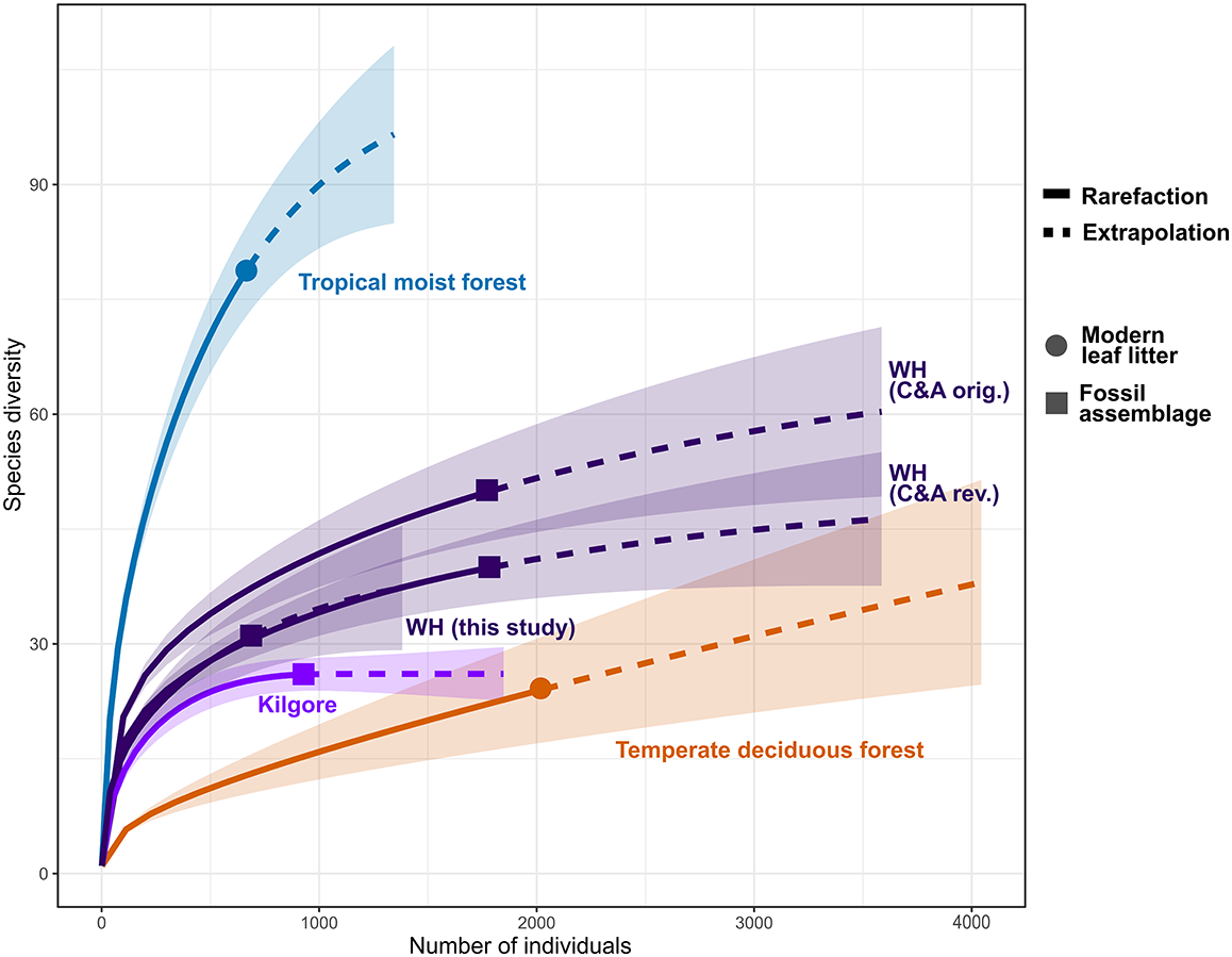


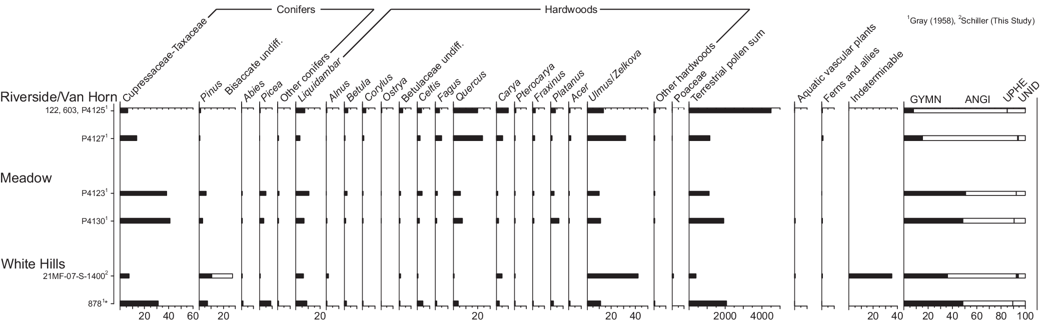


 Open access

