Attribute extraction

In the first approach, attributes are extracted from a single spectrum and visualized in elemental space to help understand the property change with the compositions. Attributes are defined as the quantitative scientific information that can be extracted from the XRD data, including metadata. Metadata store information of experimental conditions, for example, x-ray beam flux, temperature, and motor positions. From each XRD pattern [either a two-dimensional (2D) image or a 1D spectrum], several attributes can be extracted, and each of them represents a specific material property. In our recent publication,^[Reference Ren, Pandolfi, Van Campen, Hexemer and Mehta^20] we discussed several attributes that can be used to assess the global data quality, for example, crystallinity [maximum intensity (I _max) divided by average intensity (I _ave)], crystalline texture, and number of peaks. These attributes can also be used for visually segmenting the dataset. In this paper, we will introduce three additional attributes: the position of the first sharp diffraction peak (FSDP), the full-width at half-maximum (FWHM) of FSDP, and its intensity, extracted from XRD 1D spectra.

The FWHM, intensity, and position of FSDP can be identified through fitting an XRD 1D spectrum, following proper background subtraction. However, background subtraction for XRD patterns from a combi library can be challenging. Because the combi library usually covers a broad range of materials, crystalline and amorphous, multi- and single-phased, the XRD spectra may exhibit very different profiles. Scattering from the substrate and other contributions to the background can cause further difficulties. The background subtraction method also needs to be fast enough for real-time processing and can be applied to all of the spectra in a combi library without human intervention. We have chosen a multi-step method for background subtraction, and the details are included in the Supplementary Information.

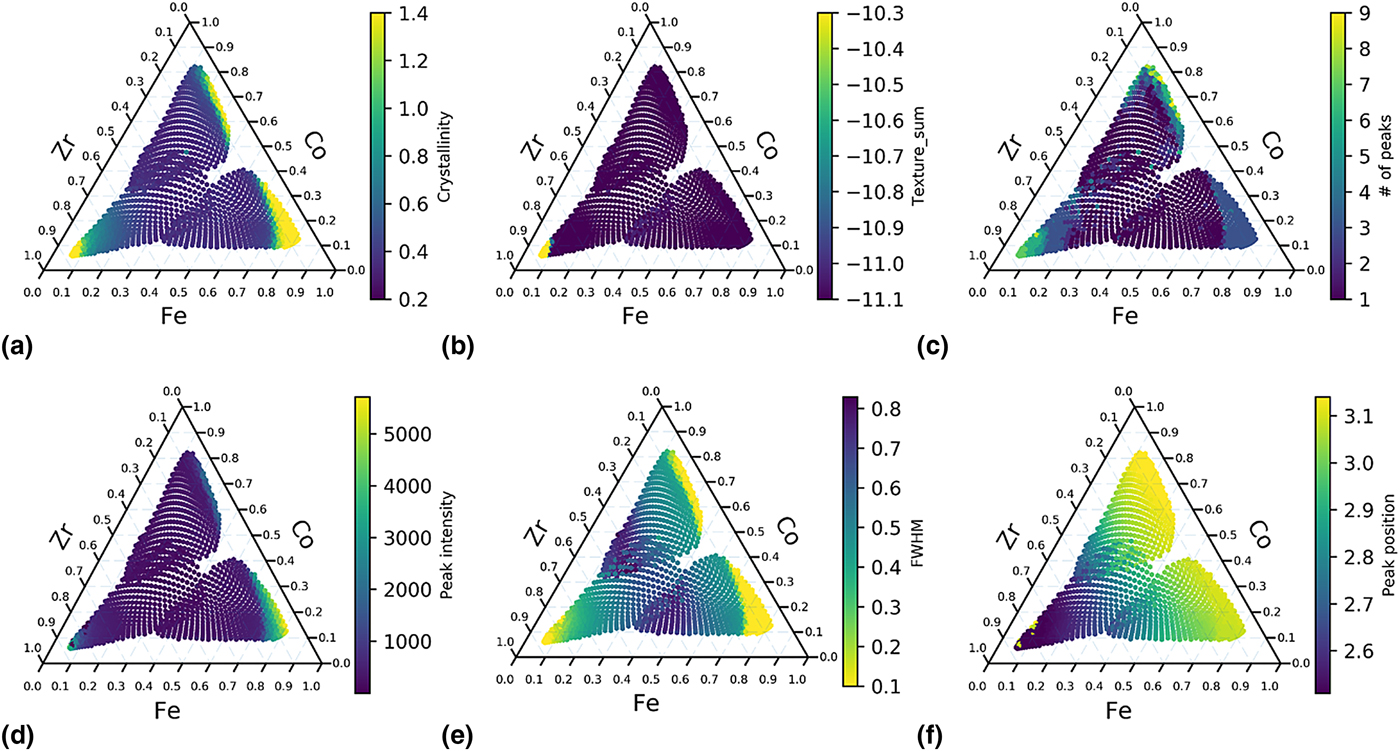
Peak fitting can then be applied to the background subtracted spectra. Based on the shape of XRD peaks, Voigt function, a convolution of Gaussian and Lorentzian functions, is often chosen to describe the shape of the XRD peaks. However, because of its high computation cost, Gaussian–Lorentzian sum (GLS) function, and GLP (Gaussian–Lorentzian product) function are often used instead.^[Reference Linford^21] In this paper, GLS will be used for fitting the XRD peaks to obtain the values for FWHM, peak position, and peak intensity. FWHM of FSDP is often used to estimate the ordered domain size in the sample, through Scherrer function.^[Reference Patterson^22] Position of FSDP can be used as a measure of the unit cell volume and to estimate material density. The intensity of FSDP can serve as a sanity check for the crystallinity (I _max/I _ave) since the maximum intensity of a spectrum can sometimes be from the background, which could falsely label a sample as being crystalline. The three attributes, FWHM, position, and intensity of FSDP, together with the other three attributes, crystallinity (I _max/I _ave), texture, and number of peaks that were discussed in our recent publication are plotted in Fig. 1 in the elemental space.

Figure 1.

Attribute mapping of Co–Fe–Zr ternary. (a) I _max/I _ave. (b) Square sum of texture. (c) Number of peaks. (d) Intensity of FSDP. (e) FWHM of FSDP. (f) Position of FSDP.

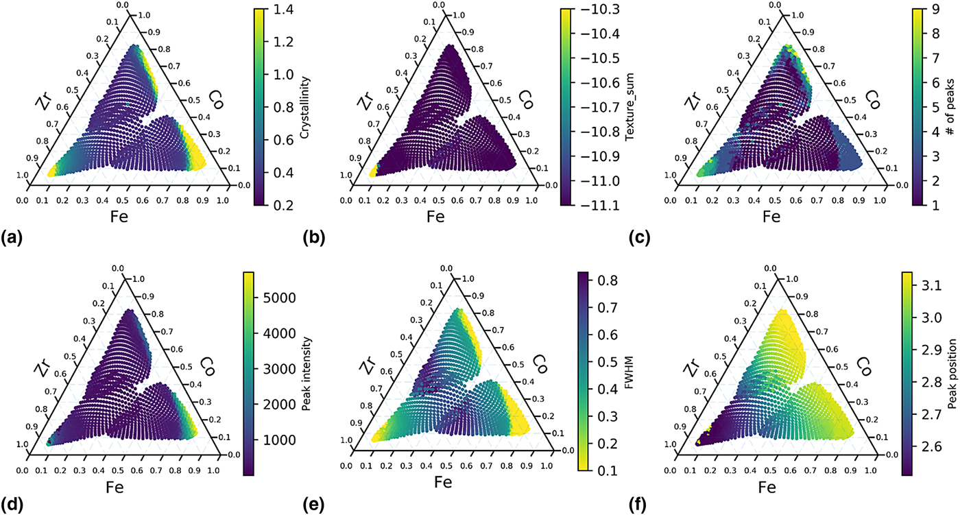
Because each of the attributes represent only one physical property, the segmentation of the dataset should be performed by taking into consideration all of the attributes. For example in Fig. 1, the sample is crystalline [Fig. 1(a) and 1(e)] but not textured [Fig. 1(b)] around Co–Fe binary region. If we only use texture attribute to segment the data, we may assume that the samples around Co–Fe binary region are the similar with those in the center of the ternary. Another example is that the peak position map [Fig. 1(f)] indicates that the spectra change gradually with the Zr concentration, which is less obvious from other attribute maps. Although it did not occur in the current library, new peaks appearing at markedly different positions in space would provide sharp visible boundaries in such mappings. By considering the six attributes, we can conclude that a potential phase boundary appears in the Zr-rich region (Zr > 60 at.%), as indicated by Fig. 1(a), 1(b), 1(c) and 1(e). Another possible phase boundary lies close to Co–Fe binary line (Zr < 15 at.%), as indicated by Fig. 1(a), 1(c) and 1(e). From the gradient seen in Fig. 1(f), we conclude that Zr concentration is a major contributor to the shift of FSDP positions.

Nearest-neighbor distance (NND)

NND approach was introduced first in our recent publication.^[Reference Ren, Pandolfi, Van Campen, Hexemer and Mehta^20] There are two major differences between this approach and attribute mapping. First, no attribute needs to be defined and extracted from the spectra in the NND approach; instead, the whole intensity array is used as raw features. Therefore, NND approach is less reliant on domain knowledge. Second, the NND approach, as its name indicates, uses not only the spectrum-of-interest, but also its nearest two neighbors in the upper stream of the measurements. One important assumption for NND approach is that XRD patterns change more dramatically (having larger distances between neighbors) across a phase boundary than within a phase region. NND often performs as well as sophisticated clustering methods even though it uses only three XRD patterns at a time, and therefore it requires much reduced memory usage and the computation cost and is significantly faster and cheaper than cluster analysis. This is especially true for large datasets. Computational resources needed for on-the-fly NND analysis of a large dataset are the same as that for a smaller dataset, whereas computational resources needed for cluster analysis scale non-linearly with the size of the dataset. Because of its low requirement on computer resources, we performed NND analysis on both 1D XRD spectra (with n features) and 2D XRD image (with n × m features for a diffraction pattern with n × m pixels) for distance mapping on a generic desktop machine in real-time. Because 2D images contain much more information than 1D spectra, such as crystalline texture, a more comprehensive analysis can be performed by using 2D images with only moderate additional computation cost. Taking the dataset shown here as an example, it took 0.03 s to calculate the neighbor distances for each 1D spectrum and 6.9 s for each 2D image on a generic desktop, while it took 30 s to collect one diffraction image. Another advantage for NND analysis is that adjacent data points on the same combi wafer share very similar backgrounds unless the wafer substrate has abrupt defects, so background subtraction is no longer a pre-requisite for NND analysis. In this study, because we used three combi wafers to cover one ternary system in order to achieve a slower composition gradient, some variances between the three wafer substrates are unavoidable. For NND analysis, these variances do not need to be taken into account. The main constraint for using this approach is that, in order to make a comparison of spectra between nearest neighbors, the scanning grids and order need to be pre-defined to ensure the physical distances between the nearest neighbors are consistent, so that the spectra are compared with their physical distances fixed. The sampling points also need to be near each other on a combi library to monitor local changes on the wafer. If the samples were chosen randomly from a wafer, the physical distances between neighbors may vary, and this approach cannot be applied anymore. A clustering method needs to be used in this case.

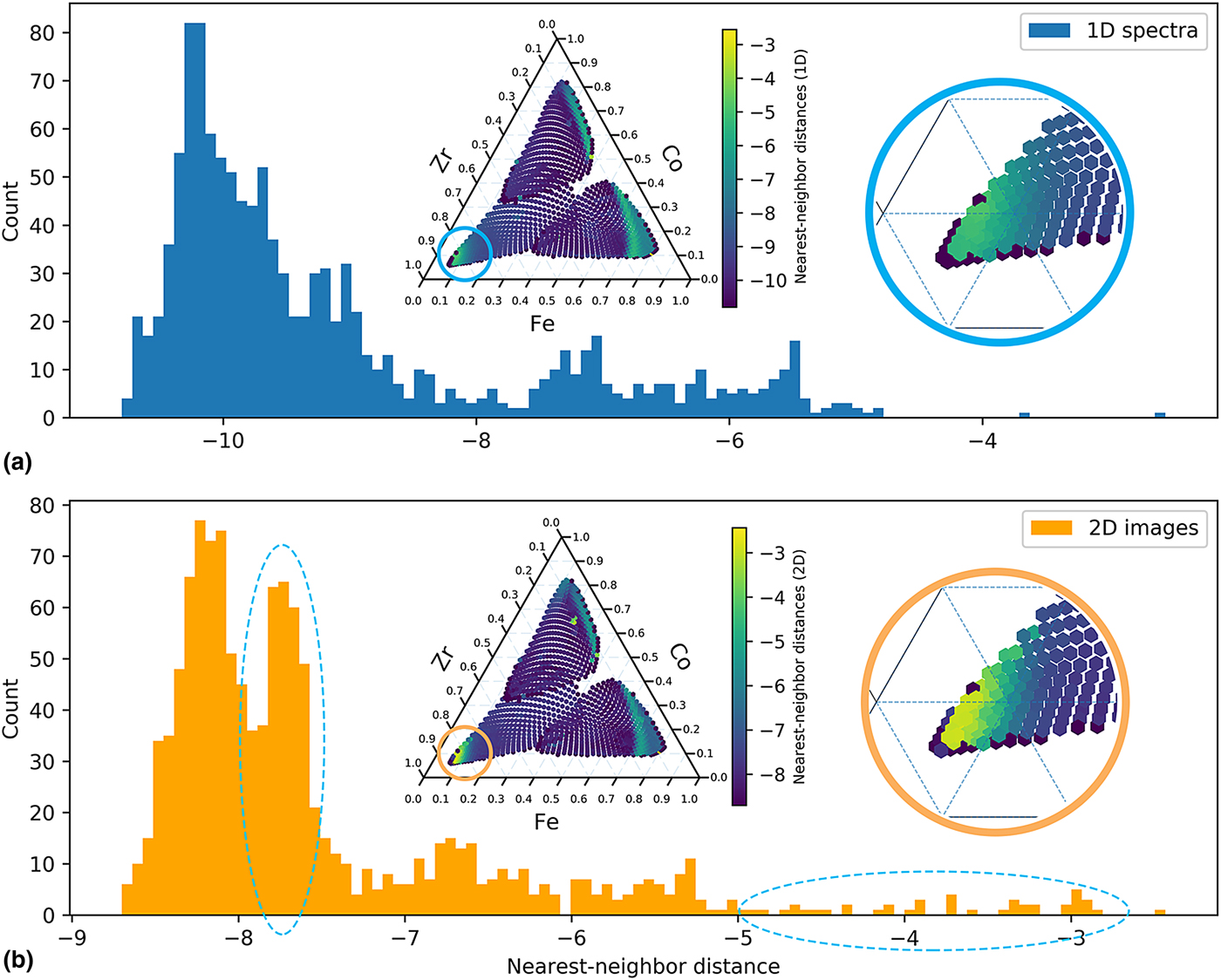
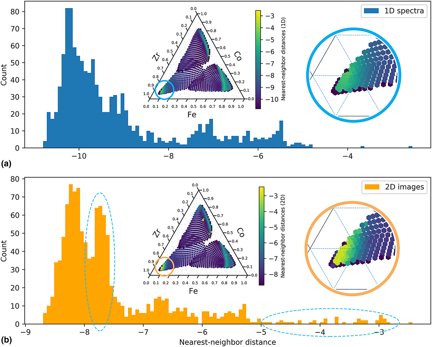
Cosine dissimilarity matrix is chosen to characterize the distances. The advantages of cosine distance matrix have been discussed in a recent paper.^[Reference Iwasaki, Kusne and Takeuchi^23] Another advantage of cosine distance matrix is that it saves the efforts to normalize the XRD intensity caused by variations in incident x-ray intensity or differences in exposure time, because cosine function only measures the angle between two vectors (spectra) in feature space, the change in absolute intensity will not impact the cosine dissimilarities. The cosine nearest-neighbor distance maps of Co–Fe–Zr ternary using both 1D spectra and 2D images are shown in the inset of Fig. 2. From Fig. 2, a potential phase boundary is observed at the Zr-rich region and along the Co–Fe binary line, which is consistent with attribute mapping in Fig. 1. We were also interested in exploring whether 2D distance maps provide more information; therefore, the distributions of the neighbor distances are plotted using histogram to elucidate the comparison between 1D and 2D NND analysis. From the histograms in Fig. 2, both distributions are extremely right skewed, because the data points within single phases that have small distances from neighbors are in majority, and the data points on the phase boundaries with large distances from neighbors are in minority. In other words, most of the XRD patterns are similar to their neighbors. The 2D image NND histogram appears to be multi-modal and more skewed compared with the 1D spectrum NND mapping, indicative of enhanced differences between neighbors for 2D images. The enhanced contrast in 2D NND is evident in the splitting of the low difference distribution and the tail at the high difference, highlighted by the two circled regions in Fig. 2. The first circle located at approximately −7.8 is due to the texture variation of the diffraction patterns from silica substrate, while the second circle from −5 to −2 is due to the rich crystalline texture in Zr-rich region (Zr > 80 at.%), where NND map of 2D images provide a higher contrast than its 1D spectrum counterpart, as shown in the magnified view in Fig. 2. We expect that for a ternary with richer texture information, the advantage of using 2D images for NND mapping will become even more obvious.

Figure 2.

NND histograms of Co–Fe–Zr ternary based on: (a) XRD 1D spectra and (b) XRD 2D Q–χ images. Inset: NND map with magnified views of Zr-rich region.

Cluster analysis

Cluster analysis has been adopted in many fields to segment large data into groups to explore trends and patterns hidden in large multi-dimensional data. There has been much progress in developing advanced phase mapping algorithms^[Reference Kusne, Gao, Mehta, Ke, Nguyen, Ho, Antropov, Wang, Kramer, Long and Takeuchi^24–Reference Suram, Xue, Bai, Le Bras, Rappazzo, Bernstein, Bjorck, Zhou, van Dover, Gomes and Gregoire^27] for multi-phased crystalline materials. However, because this paper focuses on MG and HEA systems whose XRD patterns contain much fewer numbers of peaks and much wider range of peak shapes (both amorphous and crystalline peaks), these characteristics often challenge many of the clustering approaches developed for crystalline and untextured materials. Four common clustering analysis methods^[Reference Pedregosa, Varoquaux, Gramfort, Michel, Thirion, Grisel, Blondel, Prettenhofer, Weiss, Dubourg, Vanderplas, Passos, Cournapeau, Brucher, Perrot and Duchesnay^28] have been chosen: k-medoids, density-based spatial clustering of applications with noise (DBSCAN), agglomerative clustering (hierarchical clustering), and spectral clustering. These four methods were chosen among many others because they can take pre-computed dissimilarity matrix (cosine dissimilarity is used in this case) and are scalable with large samples. K-medoids algorithm tries to minimize the distance between points labeled to be in a cluster and a point designated as the center of that cluster. In contrast to a similar and also commonly used clustering method, k-means, k-medoids works on any arbitrary dissimilarity matrices. DBSCAN algorithm treats the data as areas of high density separated by areas of low density, and thus it does not assume any particular cluster shape. The parameters for DBSCAN include the maximum distance between the core sample and its neighbors in the same cluster, and the minimum sample numbers within a cluster. The spectral clustering performs a dimensionality reduction followed by k-means in low dimensional space. The agglomerative clustering performs a hierarchical clustering using a bottom–up approach: each data point forms its own cluster, and then similar clusters are merged together. This step is repeated until the number of clusters is the same as specified. K-medoids, spectral clustering, and agglomerative clustering require the number of clusters to be specified.

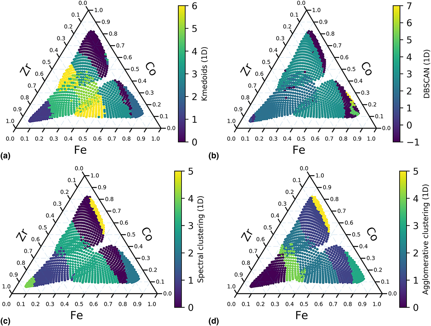
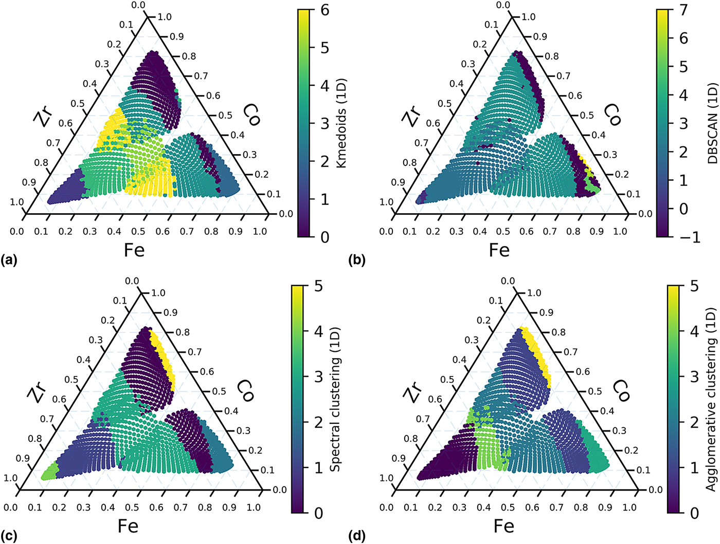
For the clustering methods that the number of clusters needs to be specified, cluster numbers ranging from 2 to 10 are examined, and the best results are shown here. K-medoids clustering [Fig. 3(a)] seems to be affected by background significantly even after automatic background subtraction, and this method runs much slower than other methods. DBSCAN [Fig. 3(b)] successfully separate out the Zr-rich and Co–Fe binary regions, but it has some unexpected artifact in Fe-rich region. Spectral clustering [Fig. 3(c)] and agglomerative clustering [Fig. 3(d)] produce the best results. Both methods pick out the potential phase boundary along Co–Fe binary line, and spectral clustering also identify the phase boundary in Zr-rich region, which are consistent with the other two methods. Both these methods also indicate that the spectra change in regions close to the center of the ternary, and additional possible boundaries that are paralleled to the Co–Fe binary line are observed. This observation was not obvious from attribute mapping or nearest-neighbor distance mapping.

Figure 3.

Clustering of 1D spectra of XRD results of Co–Fe–Zr. (a) K-medoids (n_clusters = 7) using 1D spectra. (b) DBSCAN (eps = 0.0009, min_sample = 5) using 1D spectra. (c) Spectral clustering (n_clusters = 6) using 1D spectra. (d) Agglomerative clustering (n_clusters = 6, linkage = ‘average’) using 1D spectra.

From the NND mapping using 2D images, we know that 2D images contain more information than 1D spectra, and 2D image NND mapping has higher contrast as seen in Fig. 2. The 2D Q–χ images have 1000 × 1000 pixels, and a whole dataset will have 10⁹ features, but a generic computer will not be able to handle. Therefore, in order to perform 2D cluster analysis on commodity hardware, the images need first be compressed. Second, the clustering results are highly dependent on the background subtraction method, but a 2D background subtraction method is still unavailable and difficult to develop. Therefore, the NND method is more suitable for 2D image segmentation because it only need three patterns at a time and does not require background subtraction.

Summary of segmentation approaches

Within an experimental cycle, all three approaches should be used together as an on-the-fly analysis routine for segmenting XRD patterns, because each of them has some advantages over the others. In the first approach, each attribute represents a particular material characteristic and needs to be defined and constrained carefully by an expert. Therefore, attribute extraction requires the most domain knowledge, but it also provides the most physical insights. Attribute mapping also serves as a partial ground truth for NND and cluster analysis. In the second approach, for each sample in the dataset, the sum of cosine distances of its closest neighbors is recorded. It requires less human effort because the spectra are used directly as inputs without any feature extraction or background subtraction; however, this approach only works when the scanning grids and order are pre-defined. It also does not work well for sparse scanning since the neighbors will be far away from each other, and the NND results will not provide local information anymore. But, because this approach only works with three spectra at a time and does not require background subtraction, 2D XRD images, which contain more information than 1D spectra, can be used for segmentation as the data is collected. The NND approach can be used as a first estimate of a phase map. In the last approach, spectral clustering and agglomerative clustering methods produced the best results. The clustering approach requires minimal domain knowledge and often extracts information that is not seen in attribute mapping or NND analysis; they are bench-marks for unsupervised analysis of large datasets. However, they require more computer resources, a careful background subtraction, and cannot work with 2D images on commodity computers.

Expert analysis

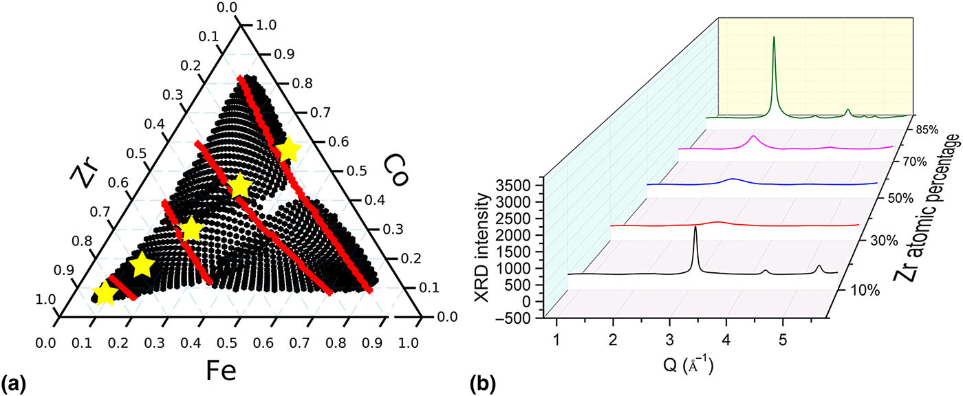
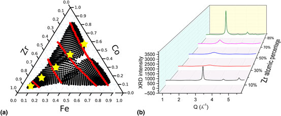
Based on the three segmentation approaches, the XRD dataset of Co–Fe–Zr ternary is segmented according to the red lines shown in Fig. 4(a). We also know that the spectrum changes more obviously with Zr composition than Co and Fe compositions. Note that in order to confirm the phase boundaries, the spectra from each side of the possible boundary need to be examined carefully. However, the primary focus of this work is to use a set of tools to provide the scientists with preliminary results during data acquisition by providing “real time” suggestions of possible regions for further analysis and investigation. The exact phase mapping of materials-of-interest is out of scope of the current manuscript. For the MG samples studied in this paper, it is most important to generate a classification of each observed composition as being amorphous or crystalline with the help of the segmentation results provided by the three approaches. Five samples were then chosen to represent this dataset, at Co : Fe = 1.5 and Zr = 10, 30, 50, 70, and 85 at.%. Their positions are marked by yellow stars in Fig. 4(a) and their spectra are shown in Fig. 4(b). By examining representative diffraction patterns from each segmented region, we were able to quantify the degree of crystallinity of each region. Along the Co–Fe binary for low Zr concentrations, sharp diffraction peaks indicative of crystalline phases are present. The bands in samples along Co–Fe binary region were found to contain a single BCC phase with a FSDP Q position of ~3.1 Å⁻¹. Two small peaks centered at about 2.0 and 3.5 Å⁻¹ in Q are from the silicon substrate, which can be observed from all of the spectra. The Fe–Co phase diagram is known to contain a large BCC solid solution region spanning from pure Fe to 80 wt.% Co.^[Reference Hunter, Osborn, Wang, Kazantseva, Hattrick-Simpers, Suchoski, Takahashi, Young, Mehta, Bendersky, Lofland, Wuttig and Takeuchi^29] When Zr atomic concentration increases above 30 at.% but below 50 at.%, the peak profiles broaden, indicating glass formation from all the three elements. At 70 at.% Zr, the diffraction peaks are broader than typical crystalline peaks but not as broad as those in the glass-forming region at lower Zr concentration. Therefore, those samples may be classified as partially crystalline. Finally at 85 at.% Zr, the samples are observed to be crystalline again. The Zr-rich corner appears to also contain a BCC phase^[Reference Jain, Ong, Hautier, Chen, Richards, Dacek, Cholia, Gunter, Skinner, Ceder and Persson^30] with the primary peak located at 2.5 Å⁻¹, both Co and Fe are known to stabilize BCC Zr, although the largest solubility for either element is merely 10 at.%. Expert analysis performed on these five samples indicates that many of the compositions in this library are not the ground-state equilibrium structure. The largest change in this ternary is from a crystalline solid-solution near the Co–Fe binary to another crystalline phase toward Zr-rich region, separated by a large region of slowly changing poorly crystalline and amorphous region. A portion of the crystalline region with high Zr centration also has noticeable preferred orientation (texture). Many aspects of this expert analysis are captured in maps produced via all three approaches, but especially so in NND map from the 2D images, agglomerative, and spectral clustering.

Figure 4.

(a) Phase boundary in Co–Fe–Zr ternary and five representatives. (b) XRD spectra for the five representatives.

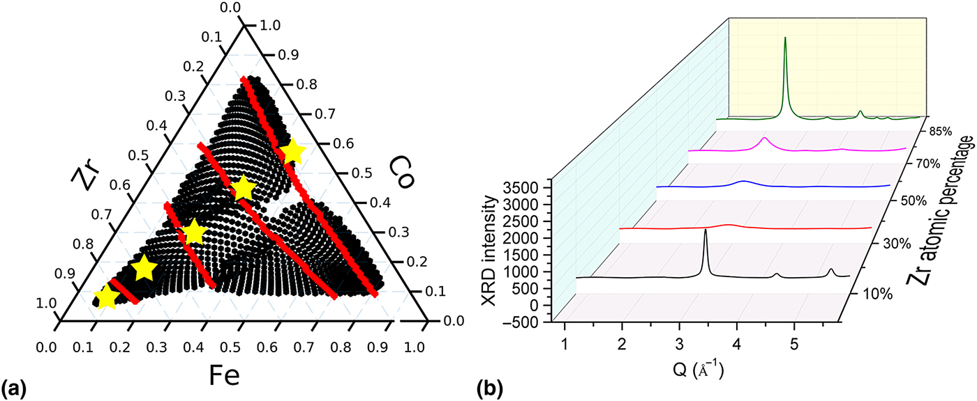
Here, we employed a series of segmentation approaches to analyze the diffraction dataset. Instead of individually examining more than 1200 individual diffraction patterns, only a handful of patterns (five in this case study) were needed to understand the morphological changes such as glass-formation and texture in the different regions. By applying this integrated on-the-fly segmentation approach to large XRD dataset, at the end of an experimental cycle, instead of having large quantity of data to analyze for months, scientists are now provided with some preliminary conclusions from the dataset. They can then focus their efforts on the most representative data and work on the dataset more efficiently.