

1. Introduction
Convective heat transfer is omnipresent in nature and industrial applications and can be divided into turbulent convection and laminar convection based on flow patterns. With increasing demand for high-parameter, high-efficiency and compact heat exchangers in thermodynamic applications, such as heat pumps, supercritical water- or  $\textrm {CO}_2$-cooled nuclear reactors for power plants, supercritical
 $\textrm {CO}_2$ solar power systems and regenerative cooling systems for rockets and scramjet engines, there is growing interest in utilising fluids at supercritical pressure (SCP) as the working medium (Huang et al. Reference Huang, Wu, Sunden and Li2016). These SCP fluids with high heat transfer capacity could substantially improve the compactness and efficiency of devices and systems. However, SCP fluids have significant differences from conventional fluids in heat transfer and flow characteristics owing to their peculiar thermodynamic behaviours. At pressures above the critical pressure, there is no distinct phase-change progress. Instead, the specific volume of the substance continually increases, and at all times there is only one phase present (Cengel and Boles Reference Cengel and Boles2014). However, the fluid properties exhibit a sharp variation within a very narrow temperature range across the pseudocritical point, resulting in distinctive flow and heat transfer behaviour, which leads to many difficulties in the design of supercritical fluid heat exchangers. Accordingly, investigating and revealing the mechanism of SCP fluid flow and heat transfer is important.
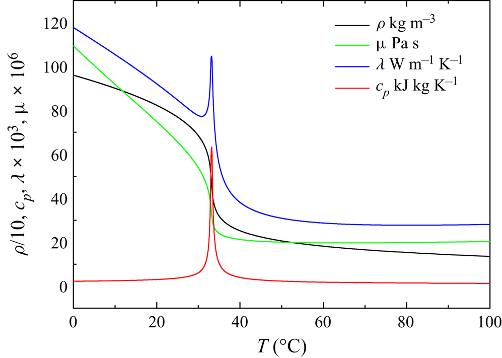
The SCP fluid flow and heat transfer capacity are closely related to fluid thermodynamic behaviours, especially thermophysical property changes near the pseudocritical temperature,  $T^*_{pc}$, which is defined as that temperature where the specific heat reaches its peak in a supercritical isobaric process. Figure 1 shows the variation in the thermophysical properties of
 $\textrm {CO}_2$ at 7.75 MPa. As the fluid temperature exceeds
 $T^*_{pc}$, the density, thermal conductivity and dynamic viscosity decrease rapidly, while the specific heat at constant pressure shows a peak at
 $T^*_{pc}$ (=306.35 K at 7.75 MPa). Owing to the substantial decrease in the density of
 $\textrm {CO}_2$ with small changes in temperature, a non-uniform density distribution arises along the heated or cooled vertical tube in the tube cross-section. Buoyancy and thermal acceleration caused by the density difference make the SCP fluid flow and convective heat transfer very complicated, which is quite different from conventional heat transfer at subcritical pressures. There have been numerous studies on the flow and heat transfer performances of supercritical fluids (Krasnoshchekov et al. Reference Krasnoshchekov, Protopopov, Van and Kuraeva1964; Hall & Jackson Reference Hall and Jackson1969; Ackerman Reference Ackerman1970; Bourke et al. Reference Bourke, Pulling, Gill and Denton1970; Petukhov Reference Petukhov1970; Shiralkar & Griffith Reference Shiralkar and Griffith1970; Hall Reference Hall1971; Hiroaki et al. Reference Hiroaki, Ayao, Masaru and Nuchi1973; Grigoriev, Polyakov & Rosnovsky Reference Grigoriev, Polyakov and Rosnovsky1977; Protopopov Reference Protopopov1977; Jackson & Hall Reference Jackson and Hall1979a,Reference Jackson and Hallb; Kurganov & Kaptil'ny Reference Kurganov and Kaptil'ny1992; Jackson Reference Jackson2002, Reference Jackson2009, Reference Jackson2013; Jackson, Evans Lutterodt & Weinberg Reference Jackson, Evans Lutterodt and Weinberg2003; Jiang et al. Reference Jiang, Zhang, Xu and Shi2008a,Reference Jiang, Zhang, Zhao and Shib; Jiang, Li and Zhao (Reference Jiang, Li and Zhao2009a); Jiang et al. Reference Jiang, Zhao, Shi, Chen and Ambrosini2009b, Reference Jiang, Xu, Li and Zhao2010; Jiang, Zhao & Liu Reference Jiang, Zhao and Liu2012; Li et al. Reference Li, Jiang, Zhao and Zhang2010; Jiang et al. Reference Jiang, Liu, Zhao and Luo2013; Peeters et al. Reference Peeters, Pecnik, Rohde, Van Der Hagen and Boersma2016; He, He & Seddighi Reference He, He and Seddighi2016; Xu, Luo & Jiang Reference Xu, Luo and Jiang2017).
Thermophysical properties of  $\textrm {CO}_2$ at 7.75 MPa.

Early experimental research on SCP fluid heat transfer was initiated in the 1950s and 1960s for the purpose of designing SCP fossil-fueled power plants and supercritical water-cooled nuclear reactors for power plants. Researchers performed experiments at SCP using water,  $\textrm {CO}_2$ or other fluids flowing in heated tubes to obtain wall temperature and heat transfer coefficient. According to these early experiments, turbulent heat transfer to supercritical fluids has very complicated features, different from those of subcritical-pressure fluids. Anomalous heat transfer phenomena occur in heated vertical tubes, both degradation and recovery in upward flows and enhancement in downward flows have been observed (Krasnoshchekov et al. Reference Krasnoshchekov, Protopopov, Van and Kuraeva1964; Petukhov Reference Petukhov1970; Hall Reference Hall1971; Grigoriev et al. Reference Grigoriev, Polyakov and Rosnovsky1977; Protopopov Reference Protopopov1977; Jackson & Hall Reference Jackson and Hall1979a,Reference Jackson and Hallb; Jackson Reference Jackson2002, Reference Jackson2009, Reference Jackson2013; He et al. Reference He, He and Seddighi2016). Shiralkar & Griffith (Reference Shiralkar and Griffith1970) found that for supercritical
 $\textrm {CO}_2$ heat transfer at high heat fluxes, degradation occurred when
 $T^*_{pc}$ was lower than the wall temperature and higher than the bulk temperature. Ackerman (Reference Ackerman1970) conducted heat transfer experiments of water at SCP in vertical tubes for different pressures, mass fluxes, heat fluxes and tube diameters, revealing that all these factors affect heat transfer at SCP as well as the bulk temperature owing to large density changes across
 $T^*_{pc}$. Hall & Jackson (Reference Hall and Jackson1969), Jackson et al. (Reference Jackson, Evans Lutterodt and Weinberg2003) and other investigators (Bourke et al. Reference Bourke, Pulling, Gill and Denton1970; Hiroaki et al. Reference Hiroaki, Ayao, Masaru and Nuchi1973) performed downward flow heat transfer experiments under otherwise identical conditions, concluding that the anomalous behaviour of heat transfer to SCP fluids was caused by buoyancy forces. Hall & Jackson (Reference Hall and Jackson1969) also associated the deteriorated heat transfer with the modification of the shear stress distribution, which gives a theoretical explanation of the mechanism of deteriorated heat transfer. Petukhov, Polyakov & Launder (Reference Petukhov, Polyakov and Launder1988) proposed that there are at least two ways to influence convective heat transfer. The direct way is through the interactions between the density fluctuations and the flow field, which serves as an additional source of turbulent kinetic energy, while the indirect effect results from the distorted flow field, which changes the magnitude of turbulence production through shear as the main source in wall shear flows. Kurganov & Kaptil'ny (Reference Kurganov and Kaptil'ny1992) found that buoyancy combined with acceleration as well as a mean negative pressure gradient significantly affected the flow and heat transfer, in the course of which the velocity fields and shear stress distribution changed. They also found that an M-shaped velocity profile occurred in upward flows and contributed to heat transfer enhancement. Shiralkar & Griffith (Reference Shiralkar and Griffith1970) and Jackson et al. (Reference Jackson, Evans Lutterodt and Weinberg2003) found that heat transfer could also be degraded by acceleration of the bulk flow as a result of thermal expansion along the tube with a negative density gradient, termed thermal acceleration. Jiang et al. (Reference Jiang, Zhang, Xu and Shi2008a,Reference Jiang, Zhang, Zhao and Shib, Reference Jiang, Li and Zhao2009a,Reference Jiang, Zhao, Shi, Chen and Ambrosinib, Reference Jiang, Xu, Li and Zhao2010, Reference Jiang, Zhao and Liu2012, Reference Jiang, Liu, Zhao and Luo2013) and Li et al. (Reference Li, Jiang, Zhao and Zhang2010) conducted a series of experiments and numerical simulations on the convective heat transfer of SCP
 $\textrm {CO}_2$ in vertical tubes and porous structures. The flow and heat transfer of SCP fluid in tubes with diameters of 2, 1, 0.27 and 0.0992 mm were studied. Xu et al. (Reference Xu, Luo and Jiang2017) proposed a new method to identify the onset of degradation caused by buoyancy effects in upward flows. Owing to the complicated mechanism of SCP flow and heat transfer, accurate prediction is significantly difficult. The main challenge is to predict turbulent behaviour under drastic thermophysical property variations. Therefore, it is necessary to investigate how turbulence is influenced by thermophysical property variations and how turbulent behaviour interacts with convective heat transfer. However, the present experimental data are not even adequate for the understanding of the heat transfer mechanism at supercritical pressure, more detailed information on velocity profiles and flow structures is needed.
To investigate how the thermophysical property variations influence turbulence, numerical studies are needed to obtain more detailed data on the flow field and heat transfer. He, Kim & Bae (Reference He, Kim and Bae2008) and Kim, He & Jackson (Reference Kim, He and Jackson2008) simulated SCP fluid heat transfer with different two-equation low-Reynolds-number turbulence models and found that predictions of the shear production of turbulence with different models varied considerably and that none of the selected models could produce reliable results for the buoyancy production of turbulence. Accordingly, more reliable heat transfer models can be designed, such as Nusselt-number relations and turbulence models (Peeters et al. Reference Peeters, Pecnik, Rohde, Van Der Hagen and Boersma2016). Many researchers take efforts to improve turbulence models for more accurate prediction of heat transfer upon strong buoyancy effects. Jiang, Wang & Xu (Reference Jiang, Wang and Xu2018) proposed a modified method that considers the anisotropic turbulent heat flux and improves the prediction accuracy of numerical simulation. It is necessary to use more advanced means to understand the mechanism of turbulent heat transfer and to provide theoretical support for the improvement of turbulence models. Direct numerical simulation (DNS) and large eddy simulations appear to be better methods to obtain the flow details.
Recently, several DNS studies have been performed to investigate turbulent heat transfer at SCP. Bae, Yoo & Choi (Reference Bae, Yoo and Choi2005) investigated SCP turbulent heat transfer to  $\textrm {CO}_2$ in heated vertical tubes using DNS at an inlet Reynold number of
 $Re_{ 0}=5400$ with a buoyancy effect incorporated; mean flow, turbulence statistics and heat transfer were discussed. They observed that heat transfer degradation shows high consistency with turbulence attenuation; similarly, heat transfer recovery and enhancement actually occur in the region where the turbulence is regenerated. Nemati et al. (Reference Nemati, Patel, Boersma and Pechik2015) discussed how the averaged thermophysical property inequality may have a profound effect on the turbulence activity in one forced convection case and two mixed convection cases with DNS of a heated turbulent flow at SCP. More specifically, Patel et al. (Reference Patel, Peeters, Boersma and Pechik2015) found that the strength of large-scale streaks and the flow anisotropy, which are integral parts of turbulence development, have a strong relation with variable property effects. Furthermore, Peeters et al. (Reference Peeters, Pecnik, Rohde, Van Der Hagen and Boersma2016) found that as the viscosity gradient interaction with the mean shear significantly affects the streak and streamwise vortex evolution, thermal expansion and buoyancy tend to decrease the streak coherence. These findings provide a sketchy theoretical explanation of the mechanism of supercritical heat transfer with strong thermophysical property variation, buoyancy and thermal expansion influence. However, few research reports have compared DNS results and experiments because the
 $x/d$ ratio in experiments is too large for DNS to accommodate with affordable computational cost. More reviews on the topic of supercritical heat transfer were provided by Kirillov (Reference Kirillov2000), Yoo (Reference Yoo2013) and other researchers (Polyakov Reference Polyakov1991; Bae et al. Reference Bae, Yoo and Choi2005).
Despite recent progress, how the flow and heat transfer in particular are influenced by buoyancy, thermal expansion and thermophysical property variation in heated vertical flow with SCP fluids still remains to be elucidated, especially in cases with both buoyancy and thermal expansion effects. A comprehensive understanding of the turbulent heat transfer mechanism, illuminating the coupling interaction between the buoyancy and thermal acceleration effects, is necessary to develop better heat transfer models.
In this paper, DNS is conducted to investigate the mechanism of heat transfer for SCP  $\textrm {CO}_2$ flowing in a heated vertical tube and to present a direct comparison with experimental data in a relatively long pipe to further understand the turbulent flow and heat transfer mechanism both experimentally and numerically. First, we are interested in the mean temperature and flow field and give a comparison with the present experimental data. Second, the mechanism of how the coupling effects of buoyancy and thermal acceleration influence the turbulence intensities is discussed, more specifically, the turbulence energy transport process while heat transfer is suppressed. Finally, how buoyancy and thermal acceleration affect the turbulence anisotropy and especially the turbulence structure were investigated, which are significant to turbulence energy transfer and the self-regeneration of turbulence in the near-wall region.
2. Physical mathematical model and computational method
2.1. Physical model and heat transfer conditions
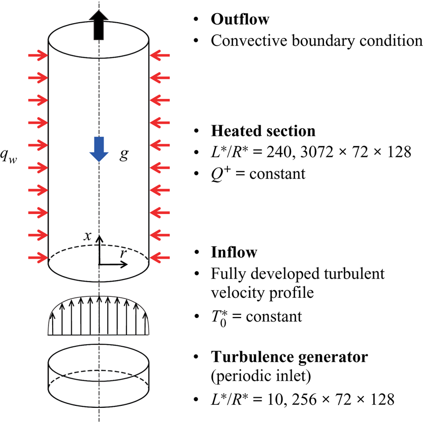
The SCP  $\textrm {CO}_2$ turbulent heat transfer in heated vertical tubes at 7.75 MPa is simulated with DNS. A schematic of the investigated geometry (with boundary conditions) is shown in figure 2. A fully developed turbulent inflow at a constant temperature
 $T^*_{ 0}$ is generated as the inlet boundary condition of the heated section. The heated section is strongly heated with a constant non-dimensional heat flux
 $Q^+$. The usual non-slip condition is adopted at the wall. For the outflow, the convective boundary condition (Orlanski Reference Orlanski1976) is specified, with the total mass conservation satisfied along the whole computational domain as follows:
 \begin{equation} \dfrac{\partial \varPhi}{\partial t}+U_c\dfrac{\partial \varPhi}{\partial x}=0, \end{equation}
where  $\varPhi$ denotes any scalar or velocity component at the outlet,
 $U_c$ is the convection velocity to which the outlet bulk velocity is assigned and
 $x$ is the coordinate in the direction of the outward normal at the boundary.
Schematic of the investigated geometry and boundary conditions (for upward flow).

2.2. Governing equations
The heated SCP  $\textrm {CO}_2$ is assumed to be at thermal equilibrium, so that the low-Mach-number assumption can be applied to simplify the energy equation (Bae et al. Reference Bae, Yoo and Choi2005). Under this assumption, we can ignore the compressibility and acoustic wave effects when we determine all thermodynamic state variables, such as density and specific heat, because the hydrodynamic pressure fluctuations are several orders of magnitude less than the thermodynamic pressure and are thus assumed to make no difference in the thermophysical property variations. We can also say that the heat transfer process considered here occurs at a thermodynamically constant pressure. This is a typical approximation for low-speed incompressibility flow heat transfer problems and has been widely used in many studies (Bae et al. Reference Bae, Yoo and Choi2005; Nemati et al. Reference Nemati, Patel, Boersma and Pechik2015; Patel et al. Reference Patel, Peeters, Boersma and Pechik2015; Peeters et al. Reference Peeters, Pecnik, Rohde, Van Der Hagen and Boersma2016).
After simplification, the conservative form of the non-dimensional governing equations in cylindrical coordinates reads as follows:
(i) the continuity equation
(2.2) \begin{equation} \frac{\partial \rho}{\partial t}+\frac{\partial (\rho u_x)}{\partial x}+ \frac{1}{r}\frac{\partial (r \cdot \rho u_r)}{\partial r}+\frac{1}{r}\frac{\partial (\rho u_\theta)}{\theta}=0; \end{equation}
(ii) the momentum equation
(2.3)\begin{align} &\frac{\partial (\rho u_x)}{\partial t}+\frac{\partial (\rho u_x \cdot u_x)}{\partial x} + \frac{1}{r}\frac{\partial (r \cdot \rho u_r \cdot u_x)}{\partial r} +\frac{1}{r}\frac{\partial(\rho u_\theta \cdot u_x)}{\partial \theta}\nonumber\\ &\quad={-}\frac{\partial p}{\partial x}+\frac{1}{{Re} }\left\{\frac{\partial}{\partial x}\left[2\mu\left(\frac{\partial u_x}{\partial x}-\frac{1}{3}\varPsi\right)\right]+\frac{1}{r}\frac{\partial}{\partial r}\left[r\cdot\mu\left(\frac{\partial u_r}{\partial x}+\frac{\partial u_x}{\partial r}\right)\right]\right. \nonumber\\ &\qquad \left.+\frac{1}{r}\frac{\partial}{\partial \theta}\left[\mu\left(\frac{\partial u_\theta}{\partial x}+\frac{1}{r}\frac{\partial u_x}{\partial \theta}\right)\right]\right\}\mp \frac{\rho}{{Fr}}, \end{align}(2.4)\begin{align} &\frac{\partial (\rho u_r)}{\partial t}+\frac{\partial (\rho u_x \cdot u_r)}{\partial x} + \frac{1}{r}\frac{\partial (r \cdot \rho u_r \cdot u_r)}{\partial r} +\frac{1}{r}\frac{\partial(\rho u_\theta \cdot u_r)}{\partial \theta}-\frac{\rho u_\theta \cdot u_\theta}{r}\nonumber\\ &\quad ={-}\frac{\partial p}{\partial r}+\frac{1}{{Re} }\left\{\frac{\partial}{\partial x}\left[\mu\left(\frac{\partial u_r}{\partial x}+\frac{\partial u_x}{\partial r}\right)\right]+\frac{1}{r}\frac{\partial}{\partial r}\left[r\cdot 2\mu\left(\frac{\partial u_r}{\partial r}-\frac{1}{3}\varPsi\right)\right]\right. \nonumber\\ &\qquad \left.+\frac{1}{r}\frac{\partial}{\partial \theta}\left[\mu\left(\frac{\partial u_\theta}{\partial r}+\frac{1}{r}\frac{\partial u_r}{\partial \theta}-\frac{u_\theta}{r}\right)\right]-\frac{1}{r}\left[2\mu\left(\frac{1}{r}\frac{\partial u_\theta}{\partial \theta}+\frac{u_r}{r}-\frac{1}{3}\varPsi\right)\right]\right\}, \end{align}(2.5)\begin{align} &\frac{\partial (\rho u_\theta)}{\partial t}+\frac{\partial (\rho u_x \cdot u_\theta)}{\partial x} + \frac{1}{r}\frac{\partial (r \cdot \rho u_r \cdot u_\theta)}{\partial r} +\frac{1}{r}\frac{\partial(\rho u_\theta \cdot u_\theta)}{\partial \theta}+\frac{\rho u_r \cdot u_\theta}{r}\nonumber\\ &\quad ={-}\frac{1}{r}\frac{\partial p}{\partial \theta}\!+\!\frac{1}{{Re}} \left\{\frac{\partial}{\partial x}\left[\mu\left(\frac{\partial u_\theta}{\partial x}+\frac{1}{r}\frac{\partial u_x}{\partial \theta}\right)\right]+\frac{1}{r}\frac{\partial}{\partial r}\left[r\cdot \mu\left(\frac{\partial u_\theta}{\partial x}+\frac{1}{r}\frac{\partial u_r}{\partial \theta}-\frac{u_\theta}{r}\right)\right]\right. \nonumber\\ &\qquad \left.+\frac{1}{r}\frac{\partial}{\partial \theta}\left[2\mu\left(\frac{1}{r}\frac{\partial u_\theta}{\partial \theta}+\frac{u_r}{r}-\frac{1}{3}\varPsi\right)\right]+\frac{1}{r}\left[\mu\left(\frac{\partial u_\theta}{\partial r}+\frac{1}{r}\frac{u_r}{\partial \theta}-\frac{u_\theta}{r}\right)\right]\right\}; \end{align}(iii) the energy equation without internal heat sources
(2.6)\begin{align} &\frac{\partial (\rho h)}{\partial t}+\frac{\partial (\rho u_x \cdot h)}{\partial x}+\frac{1}{r}\frac{\partial(r\cdot \rho u_r \cdot h)}{\partial r}+\frac{\partial (\rho u_\theta \cdot h)}{\partial \theta}\nonumber\\ &\quad =\frac{1}{{ Re }}\frac{1}{{Pr}} \left[\frac{\partial}{\partial x}\left( \lambda \frac{\partial T}{\partial x}\right)+\frac{1}{r}\frac{\partial}{\partial r}\left(r \cdot \lambda \frac{\partial T}{\partial r}\right)+\frac{1}{r}\frac{\partial}{\partial \theta}\left(\frac{1}{r}\cdot \lambda \frac{\partial T}{\partial \theta}\right)\right], \end{align}


where
 \begin{equation} \varPsi=\boldsymbol{\nabla}\cdot \boldsymbol{u} = \frac{\partial u_x}{\partial x}+\frac{1}{r}\frac{\partial (ru_r)}{\partial r}+\frac{1}{r}\frac{\partial u_\theta}{\partial \theta}. \end{equation}
The parameters  $x$,
 $r$ and
 $\theta$ are the streamwise, radial and circumferential coordinates, respectively. The parameter
 $y=1-r$, which denotes the distance from the wall, is also sometimes used. Note that
 $\theta$ is an angle from 0 to
 $2{\rm \pi}$ rather than a length. All variables in the equations are in non-dimensional form and are defined as follows:
 \begin{equation} \left. \begin{gathered} x=\dfrac{x^*}{R^*},\quad r=\dfrac{r^*}{R^*},\quad t=\dfrac{t^*}{R^*/U^*_0},\quad u_i=\dfrac{u_i^*}{U^*_0},\\ p=\dfrac{p^*}{\rho^*_0 U_0^{*2}},\quad \rho=\dfrac{\rho^*}{\rho^*_0},\quad \mu=\dfrac{\mu^*}{\mu^*_0},\quad \lambda=\dfrac{\lambda^*}{\lambda^*_0},\\ T=\dfrac{T^*}{T^*_0},\quad h=\dfrac{h^*-h^*_{pc}}{c^*_{p {\rm 0}}T^*_{ 0}} \end{gathered} \right\} \end{equation}
where the superscript  $*$ denotes dimensional quantities, the subscript 0 denotes the inlet condition,
 $R^*$ is the tube radius and
 $h^*_{pc}$ is the enthalpy at
 $T^*_{pc}$. The non-dimensional parameters shown in the governing equations are written as
 \begin{equation} {Re} =\frac{U^*_{ 0}R^*}{\nu^*_{ 0}},\quad {Pr} = \frac{\mu^*_0 c^*_{p0}}{\lambda^*_0},\quad \frac{1}{Fr}=\frac{g R^*}{ U_0^{*2}}. \end{equation}
All the thermophysical properties of  $\textrm {CO}_2$ are from the NIST database. The temperature is calculated as a function of enthalpy, and all other physical properties are calculated as a function of temperature at the thermodynamic pressure, which is constant at
 $p^*_0=7.75\ \textrm {MPa}$ in the present work. We use
 $h^*_{pc}$ rather than
 $h^*_{0}$ to define the non-dimensional form of enthalpy. This is to avoid any non-monotonic relationship between
 $\rho h$ and
 $h$ to allow a unique update
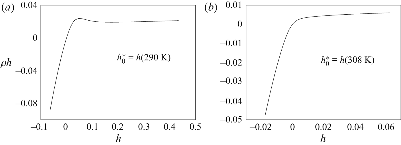
 $h=h(p_0^*, \rho h)$. Figure 3 shows the relationship between
 $\rho h$ and
 $h$ for
 $\textrm {CO}_2$ at 8.0 MPa (
 $T^*_{pc}=308 K$) using different reference enthalpies
 $h_{ 0}^*$. The line in figure 3(a) is non-monotonic, which indicates potential logical difficulties for the conservative variable
 $\rho h$ in the energy equation because one
 $\rho h$ value could be somewhere related to more than one
 $h$ value. Hence,
 \begin{equation} \left. \begin{gathered}
T^*=T(p^*_0,h^*),\\ \rho^* = \rho(p^*_0,T^*),\quad \mu^* =
\mu(p^*_0,T^*),\\ \lambda^* = \lambda(p^*_0,T^*),\quad c_p^* =
c_p(p^*_0,T^*), \end{gathered} \right\}
\end{equation}
Relationship between  $\rho h$ and
 $h$ for
 $\textrm {CO}_2$ at 8.0 MPa: (a)
 $h_0^*= h$ (290 K); (b)
 $h_0^*= h(T_{pc}^*)= h$ (308 K).

In the discussions, averaged values over time and over homogeneous circumferential direction are used to investigate mean thermophysical and velocity statistics. Favre averaging is used to define the mean quantities and the difference between the instantaneous value and the Favre-averaged value to describe the fluctuation about the Favre-averaged mean, except for temperature, which has no transport changes with density variation. Favre averaging is defined as density-weighted Reynold averaging. Its mean value,  $\tilde {\phi }$, and its fluctuation,
 $\phi ''$, are defined as follows:
 \begin{equation} \tilde{\phi}=\frac{\bar{\rho \phi} }{\bar{ \rho }},\quad \phi''=\phi-\tilde{\phi}, \end{equation}
where  $\bar {\phi }$ denotes Reynold averaging and
 $\phi$ is the instantaneous value. The mean temperature is always calculated with Reynold averaging, so the overline for averaged temperature is dropped in the following discussion.
2.3. Numerical methods and validation
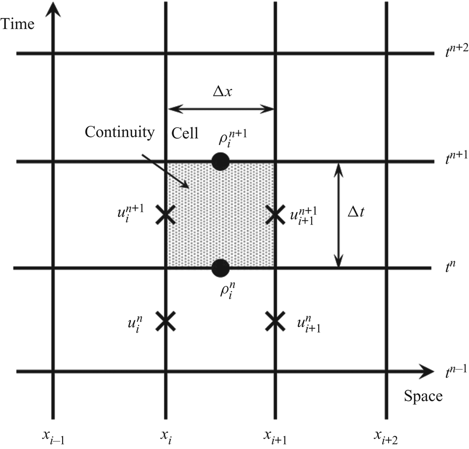
The simulation was conducted using an in-house DNS package, CHAPSim (Seddighi Reference Seddighi2011; He et al. Reference He, He and Seddighi2016). A staggered mesh was used in the simulation to solve the Navier–Stokes equations more steadily, in which all scalar variables such as density and viscosity are located at the control volume centre, while each velocity component was staggered using a one-half grid spacing and time step with respect to the scalar variables. Figure 4 indicates how the scalar variables and velocity component are located at a staggered mesh spatially and temporally. For temporal discretisation, an explicit low-storage, third-order Runge–Kutta scheme was used, while a second-order central difference scheme was used for spatial discretisation. The Poisson equation for pressure was solved using fast-Fourier transforms to ensure that continuity was satisfied, taking advantage of an imposed periodicity in both streamwise and spanwise directions.
Space–time staggered grid.

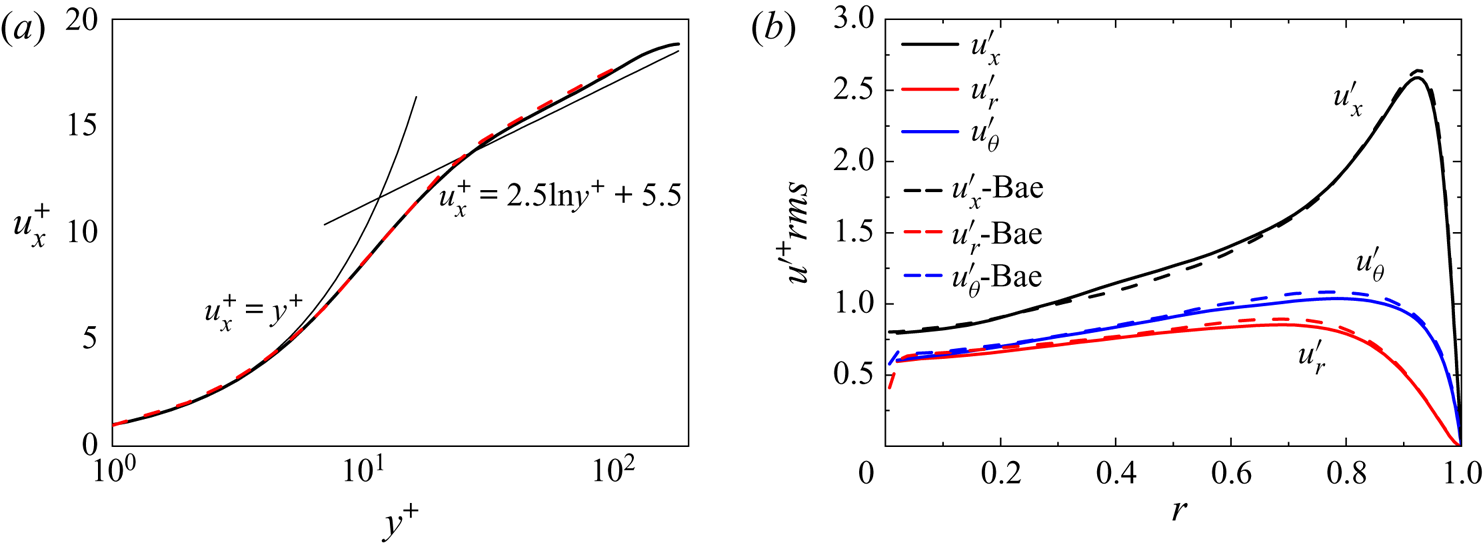
In the numerical method, the whole computational domain consists of a turbulence generator section and heated section. First, a periodic inflow turbulence generator with an axial dimension of  $L^*/R^*=10$ was applied to generate fully developed turbulence. Following this, the time-dependent velocity profile was directly copied as the turbulent inlet boundary condition for the heated pipe. Figure 5 shows the streamwise mean velocity and root mean square of velocity fluctuations of each component at
 $Re_{ 0}=5400$ using a mesh of
 $128\times 64\times 128$ along the
 $x$,
 $r$ and
 $\theta$ directions, respectively, compared with the results of Eggels et al. (Reference Eggels, Unger, Weiss, Westerweel, Adrian, Friedrich and Nieuwstadt1994) and Bae et al. (Reference Bae, Yoo and Choi2005). The good agreements indicate that the turbulence generator can generate reasonable turbulence.
Validation of velocity for the periodic inflow turbulence generator: line, present work; (a) mean flow, (- -) Eggels et al. (Reference Eggels, Unger, Weiss, Westerweel, Adrian, Friedrich and Nieuwstadt1994); (b) the root mean square of velocity fluctuation, (- -) Bae et al. (Reference Bae, Yoo and Choi2005).

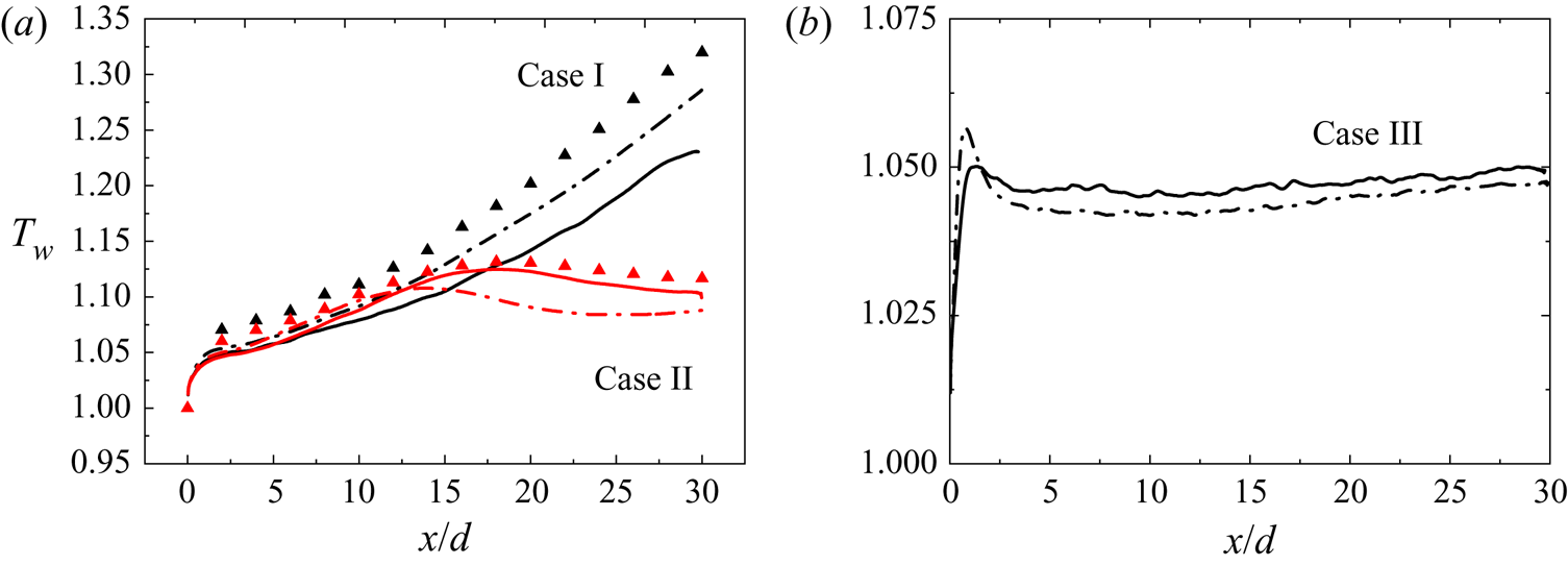
The code was validated using the DNS data from Bae et al. (Reference Bae, Yoo and Choi2005) and Chu & Laurien (Reference Chu and Laurien2016) for strongly heated SCP fluids flowing in vertical tubes both upward and downward. Figure 6 shows a comparison of wall temperature for upward and downward cases from Bae & Laurien using a mesh of  $768\times 64\times 128$ along the
 $x$,
 $r$ and
 $\theta$ directions, respectively. The present results show good agreement with both Bae & Laurien and little deviation can be observed in upward cases. A different property database was used for the computation of supercritical fluid properties, which may account for the difference.
Validation of the wall temperature of heated vertical tubes: line, present work; (- $\cdot$-) Bae et al. (Reference Bae, Yoo and Choi2005); and (
 $\blacktriangle$) Chu & Laurien (Reference Chu and Laurien2016).

2.4. Simulation conditions
Corresponding to the experiments (Wang, Jiang & Xu Reference Wang, Jiang and Xu2018), four cases were selected to be simulated using DNS under the conditions in table 2. The non-dimensional governing parameters in the table are the non-dimensional heat flux  $Q^+={q_w R^*}/{\lambda ^*_0 T^*_0}$, the inlet Grashof number
 ${Gr}_0^*={g\beta ^*_0 q_w D^{*4}}/{\nu _0^{*2} \lambda ^*_0 }$ and the inlet Reynolds number
 ${Re}_{0}={\rho ^*_0 U^*_0 D^*}/{\mu ^*_0}$ based on the inlet bulk velocity
 $U^*_0$, where the subscript 0 refers to the inlet condition and
 $D^*=2R^*$ is the tube diameter. In the simulation, for the sake of calculation costs, the non-dimensional length
 $L^*/R^*$ is set to 240 in order to investigate the heat transfer process across the pseudocritical threshold.
The simulation is conducted in both upward and downward directions to investigate the effect of buoyancy on heat transfer. Moreover, the heat fluxes are chosen to be 49 and  $78\ \textrm {kW}\ \textrm {m}^{-2}$ in the upward cases and downward cases, respectively, to compare the effects of buoyancy and thermal acceleration. As the heat flux increases, the thermal acceleration effects become stronger among the influencing factors, leading to a complicated heat transfer rule, which is entirely different from conditions under the buoyancy effects. Therefore, it is a requirement that the coupling mechanism between the thermal acceleration and buoyancy effects should be investigated.
Simulation conditions for validation, supercritical pressure  $\textrm {CO}_2$,
 $p^*_{ 0}=8.0$ MPa,
 $T^*_0=301.15\ \textrm {K}$,
 $Re_0=5400$,
 $Pr_0=3.20$.

Simulation conditions, supercritical pressure  $\textrm {CO}_2$,
 $p^*_{ 0}=7.75\ \textrm {MPa}$,
 $Re_{ 0}=3540$,
 $D^*=1 \ \textrm {mm}$.

The mesh for the heated section is  $3072\times 72\times 128$ for the
 $x$,
 $r$ and
 $\theta$ directions, respectively, with corresponding grid resolutions of
 $\Delta x^+<10$,
 $0.10<\Delta r^+<6.28$ and
 $\Delta (r\theta )^+<6.28$ at the inlet. In the axial and circumferential direction, the grids are uniform. In the radial direction, the grid spacing is non-uniform with, conveniently, a finer grid spacing near the wall with a hyperbolic tangent function. Note that a grid spacing about
 $O(0.1\eta )$ and
 $O(0.1\delta _v)$ in the radial direction is satisfied at the wall, where
 $\eta \equiv (\nu ^3/\varepsilon )^{1/4}$ is the Kolmogorov scale and
 $\delta _v\equiv \nu /u_\tau$ is the viscous length scale. A grid independence study was carried out for the supercritical pressure
 $\textrm {CO}_2$ flowing in a vertical tube. The Nusselt number with respect to
 $x/d$ was calculated for comparison. A finer mesh, e.g.
 $3456\times 96\times 192$, would incur a much longer calculation time while the difference for local Nusselt number did not exceed
 $\pm 0.1\,\%$. Moreover, based on DNS studies for supercritical pressure fluids with a similar given
 $Re_0$ from an existing numerical literature (Bae et al. Reference Bae, Yoo and Choi2005; Patel et al. Reference Patel, Peeters, Boersma and Pechik2015; Chu & Laurien Reference Chu and Laurien2016), a mesh with
 $3072\times 72\times 128$ was selected as the most appropriate mesh size. Note that for the simulation with higher
 $Q^+$ and stronger effects of buoyancy force, the non-dimensional time step is supposed to be smaller. In our simulations (cases I–IV), the minimum non-dimensional time step used was
 $3.2 \times 10^{-4}$ while
 ${\rm CFL}<1.0$ was specified to ensure time-step convergence. Turbulence statistics were not be collected until a satisfactory converged state was reached.
3. Results and discussion
The top priority of this paper is to give a direct comparison between DNS and the present experimental results; the heat transfer behaviour of the heated SCP fluid is discussed, and then the effects of buoyancy and thermal acceleration are estimated both qualitatively and quantitatively. When discussing the results, first, we investigate the mean flow profiles, including the velocity distribution and property variation in the turbulent flow. Subsequently, we focus on how exactly the local as well as global flow acceleration and thermophysical property variation produce an effect on the turbulence intensity from two aspects, namely turbulent kinetic energy and turbulent structures. A mechanism of heat transfer degradation with buoyancy and thermal acceleration effects is obtained.
3.1. Heat transfer and flow performance
3.1.1. Heat transfer and thermophysical characteristics
In the corresponding experiments, the test section was a vertical stainless steel tube which was heated by an alternating current and thermally insulated by a layer of silica wool. The inside diameter of the tube is 1 mm, the outside diameter is 2 mm. One of the data reduction methods used is based on the assumption of one-dimensional heat conduction with an internal heat source in the thin tube wall. The local temperatures of the tube outer surface,  $T^*_{w,o}(x)$, were measured by the thermocouples, and the local temperatures of the inner tube surface,
 $T^*_{w,i}(x)=T^*_w(x)$, were calculated as
 \begin{equation} T^*_{w,i}(x)=T^*_{w,o}(x)+\frac{q_v (x)}{16\lambda^*}[D_0^{*2}-D_i^{*2} ]+\frac{q_v (x)}{8\lambda^*} D_o^{*2} In \frac{D^*_i}{D^*_o} \end{equation}
in which  $D^*_o$ and
 $D^*_i$ are the outside and inside diameters of the tube
 $(\textrm {mm})$;
 $\lambda ^* =16.38 \ \textrm {W}\,(\textrm {m}\ \textrm {K})^{-1}$ is the coefficient of thermal conductivity of stainless steel; and
 $q_v$ is the heat source given by the alternating current
 $(\textrm {W}\ \textrm {m}^{-3})$. More details of the experiment methods can be found in other experimental research papers of the authors (Jiang et al. Reference Jiang, Zhang, Xu and Shi2008a,Reference Jiang, Zhang, Zhao and Shib).
In the DNS, the local Nusselt number  ${ Nu}_x$ is used to investigate the local heat transfer characteristics, which is defined with some bulk parameters on the cross-section. The bulk parameters are defined based on local bulk mass flux
 $G_b$ and local bulk enthalpy
 $h_b$:
 \begin{gather} G_b=\dfrac{1}{A} \int_{A} \overline{\rho u_x} \,\textrm{d}A, \end{gather}
 \begin{gather} h_b=\dfrac{1}{G_bA} \int_{A} \overline{\rho u_x h} \,\textrm{d}A. \end{gather}
The bulk temperature is calculated as a function of enthalpy and thermodynamic pressure; bulk density and bulk velocity are then calculated as
 $$\begin{gather} T^*_b=T(p^*_0,h^*_b), \end{gather}$$
 $$\begin{gather}\rho^*_b=\rho(p^*_0,T^*_b), \end{gather}$$
 $$\begin{gather}U_b=\dfrac{G_b}{\rho_b}. \end{gather}$$
Consequently, the local heat transfer coefficient,  $\alpha (x)$, at each axial location was calculated as
 \begin{equation} \alpha^* (x)=\frac{q_w}{T^*_{w}(x)-T^*_{b}(x)}. \end{equation}
The local Nusselt number was defined as
 \begin{equation} { Nu}_x=\frac{\alpha^* (x) D^*}{\lambda^*_{b} (x)} \end{equation}
in which  $\lambda ^*_{b} (x)$ is the coefficient of thermal conductivity based on the bulk temperature of the fluid.
In the simulations, the wall temperature exceeds  $T^*_{pc}$, thus, almost immediately, the fluid in the near-wall section is heated to
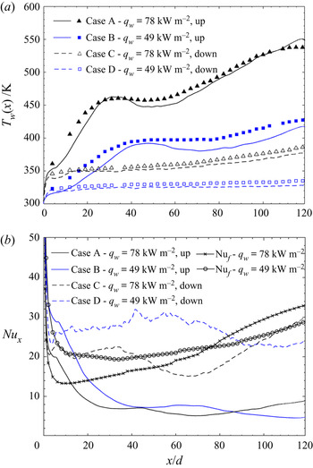
 $T^*_{pc}$. Figure 7 shows the distributions of the wall temperature
 $T^*_{w}(x)$ and the local Nusselt number
 ${ Nu}_{x}$ in the streamwise direction. As shown in figure 7(a), there is good agreement between the DNS results and the experimental data, both of which show an anomalous peak of wall temperature in the upward flows of Cases A and B. The higher the heat fluxes, the more sharply the peak wall temperature increases. However, in the downward flows for Cases C and D. No significant increases in temperature or wall temperature peaks were observed.
Streamwise distributions of mean wall temperature and local Nusselt number for Cases A to D: (a)  ${T_w}(x)=\overline {T^*_w(x)}$; lines indicate results from DNS; dots indicate results from experiments (Wang et al. Reference Wang, Jiang and Xu2018); (b)
 ${ Nu}_x$ from DNS compared with
 ${ Nu}_f$ with the (3.9)–(3.14).

Figure 7(b) shows the distributions of the local Nusselt number  ${ Nu}_{x}$ from DNS, according to which a significant decrease in
 ${ Nu}_{x}$ is shown in Cases A and B and a slight reduction appears in Cases C and D. Because
 ${ Nu}_{x}$ is the non-dimensional number representing the intensity of heat transfer, its distribution is consistent with the heat transfer behaviour observed in the temperature distribution in figure 7(a). Figure 7(b) shows the comparison of the local Nusselt number
 ${ Nu}_{x}$ from DNS with the local Nusselt number
 ${ Nu}_{f}$ of forced convection heat transfer, which is calculated with the empirical correlation without consideration of the influence of buoyancy and thermal acceleration proposed by Krasnoshchekov et al. (Reference Krasnoshchekov, Protopopov, Van and Kuraeva1964), Grigoriev et al. (Reference Grigoriev, Polyakov and Rosnovsky1977) and Protopopov (Reference Protopopov1977):
 \begin{equation} \frac{ Nu_{ 0}}{{ Nu}_f(x/d)}=\frac{1}{F_{ TD}(x/d)F_{ \nu 2}(x/d)}, \end{equation}
where  $F_{ TD}$ gives the entrance effect
 \begin{equation} F_{ TD}=1+2.35Pr^{{-}0.4}Re_f^{{-}0.15}(x/d)^{{-}0.6}\textrm{exp}({-}0.39Re_f^{{-}0.1}\cdot x/d). \end{equation}
The factor  $F_{\nu {\rm 2}}$ modifies the effect of non-uniform properties as
 \begin{equation} F_{\nu {\rm 2}}=\left(\frac{\rho^*_w}{\rho^*_b}\right)^{0.4}\cdot \left( \frac{\overline{c^*_p}}{c^*_p}\right)^n. \end{equation}
If  $\overline {c^*_p}/c^*_{pb} > 1$,
 $n=0.7$.
If  $\overline {c^*_p}/c^*_{pb} < 1$,
 \begin{equation} \left.
\begin{array}{ll@{}} n=0.4 & T^*_w< T^*_{pc} \ {\rm or} \
T^*_b\geq 1.2T^*_{pc},\\
n=n_1=0.22+0.18(T^*_w/T^*_{pc}) & T^*_b< T^*_{pc} \ {\rm and} \
1< T^*_{w}/T^*_{pc}<2.5,\\ [2pt]
n=n_1+(5n_1-2)(1-(T^*_b/T^*_{pc})) & 1\leq T^*_b<1.2.
\end{array} \right\}\end{equation}
The following expression for  $Nu_0$ was proposed by Gnielinski (Reference Gnielinski1976):
 \begin{gather} { Nu_0}=\frac{\left({\zeta}/{8}\right)(Re -1000)Pr}{1+12.7\sqrt{\zeta/8}(Pr^{2/3}-1)}, \end{gather}
 \begin{gather} \zeta=\frac{1}{(1.82\log_{ 10}{Re}_b-1.64)^2}. \end{gather}
The comparison between  ${ Nu}_x$ and
 ${ Nu}_f$ shows the heat transfer characteristics of mixed convection under the coupling effects of buoyancy and thermal acceleration. In downward flows, the direction of buoyancy effects is opposite the direction of flow and thermal acceleration. The local Nusselt number
 ${ Nu}_x$ is larger than
 ${ Nu}_f$ at
 $x/d<52$ for Case C and at
 $x/d<90$ for Case D with a little decrease in the latter part of the tube, which means that the mixed heat transfer is enhanced by the buoyancy force at first but degrades as thermal acceleration takes place in the downstream section in downward flows. Owing to the help of buoyancy effects, in the downward flow, a valley temperature value even appears at the very beginning because the heat transfer is strengthened locally. However, for upward flows,
 ${ Nu}_x$ is much less than
 ${ Nu}_f$ after the entry section for both Case A and Case B. Significant heat transfer degradation occurs in the inlet region immediately, and then heat transfer recovers to some extent, after which additional degradation occurs. The complicated heat transfer phenomenon of downward flow and upward flow is not merely due to the property variation in the supercritical fluid but also controlled by the coupling effect of buoyancy and thermal acceleration, as discussed later.
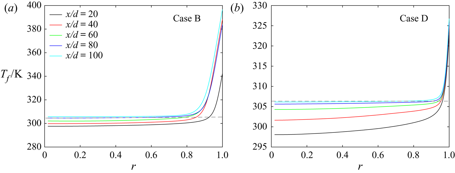
As figure 8 shows, for the low heat flux, the fluid in the near-wall region is heated across the pseudocritical point at  $x/d=10$, while the temperature of the fluid in the centre of the tube is lower than
 $T^*_{pc}$ (=306.35 K). As the downstream bulk temperature is heated to approach
 $T^*_{pc}$, the pseudocritical point, where fluid transforms to the supercritical state, gradually moves to the core region. At
 $x/d>80$, almost all fluid in the cross-section is heated to above
 $T^*_{pc}$, the flow is thoroughly transformed to the supercritical state, with extremely low viscosity and density. The non-uniform temperature distribution leads to a non-uniform thermophysical property distribution in the cross-section as well as in the streamwise direction.
Mean fluid temperature distributions for (a) Case B and (b) Case D. The grey dashed line indicates  $T^*_{pc}=306.35\ \textrm {K}$ at 7.75 MPa.

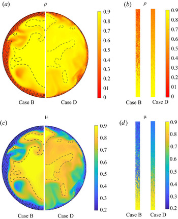
As the fluid is heated to the supercritical state, the property variation is significant. Figure 9 shows the instantaneous cross-sectional distribution of non-dimensional density and viscosity in the corresponding cases. As seen in these figures, the density and dynamic viscosity vary violently in the near-wall region and decrease with a significant gradient in the axial direction. The property variation in the downward flow is less violent than in the upward flow. The density gradient in the downward flow is smaller in the near-wall region than in the upward flow. This can be attributed to the fact that the temperature is more uniform in the downward flow.
Distribution of instantaneous density and viscosity for (a,c) Case B and (b,d) Case D: (a,c) for the horizontal cross-section at  $x/d=40$; (b,d) for the vertical cross-section at
 $r=0.85$. Note that temperature contours are drawn with dashed lines.

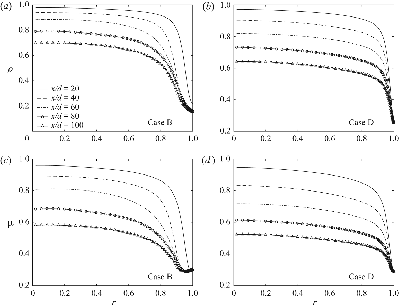
Figure 10 shows the mean profiles of non-dimensional density and viscosity distributions. The strongest variation occurs close to the wall. The property gradient is much larger near the wall than at the centre of the tube. Owing to the steep density gradients in the axial and radial directions, both global flow acceleration and local buoyancy forces are developed in the streamwise direction. The significant decrease in density and thermal conductivity not only has a direct effect on the heat transfer ability but also triggers a series of perturbations in turbulence development.
Distributions of mean density and viscosity in the cross-section at different locations for Cases B and D.

The global flow acceleration driven by the temperature gradient in the axial direction is called thermal acceleration. Mceligot & Jackson (Reference Mceligot and Jackson2004) suggested that this aspect plays an important role in the attenuation of turbulent flow and defined a non-dimensional factor  ${Kv}={4q_wD^*\alpha ^*_p}/{{Re}^2\mu ^* c^*_p}$ to to express the effect. According to their experiment results, they stated that if
 ${Kv}>9.5\times 10^{-7}$, the thermal acceleration leads to heat transfer degradation. The author and his team (Jiang et al. Reference Jiang, Liu, Zhao and Luo2013) found that in a micro tube of tube diameter
 $D^*=0.0992\ \textrm {mm}$, the flow acceleration caused by a pressure drop is approximately equivalent to that caused by thermal expansion. Therefore, the influence of a pressure drop should be considered in the evaluation of flow acceleration in a micro channel with
 ${Kv}={Kv_p+Kv_T}$, where
 ${Kv_p}$ and
 ${Kv_T}$ represent flow acceleration factors caused by thermal expansion and pressure drop, respectively. When
 ${Kv}>5.5\times 10^{-7}$, the flow acceleration caused by thermal expansion and pressure reduction inhibits the development of turbulence, weakens the generation of turbulent kinetic energy, and reduces the heat transfer capacity.
To measure the effect of the buoyancy effect, a non-dimensional factor  $Bo^*={Gr^*}/ {Re^{3.425 }Pr^{0.8}}$ was defined by Jackson & Hall (Reference Jackson and Hall1979a,Reference Jackson and Hallb), where
 ${Gr}^*={\rho ^* g D^{*4} q_w}/{\lambda ^* \nu ^{*2}}$ denotes the local Grashof number based on bulk properties and tube diameter. Jackson stated that if
 ${Bo^*<6.0\times 10^{-7}}$, the effect of buoyancy can be ignored; for upward flow, if
 $6.0\times 10^{-7}<{Bo^*}<1.2\times 10^{-6}$, the buoyancy force starts to weaken the heat transfer; if
 $1.2\times 10^{-6}<{Bo^*}<8.0\times 10^{-6}$,
 $Nu$ starts to recover but is still lower than
 ${ Nu}_f$; if
 $8.0\times 10^{-6}<{Bo^*}$, the buoyancy force is very strong, which disrupts the turbulence and enhances the convective heat transfer. According to experimental research and theoretical analysis, the author's team obtained the influence law of the floating lift force and flow acceleration in the small tube on the convective heat transfer of SCP
 ${\textrm {CO}_2}$. If
 ${Bo^*}<2.0\times 10^{-7}$, the influence of buoyancy can be neglected for both upward and downward flow. For upward flow with
 $2.0\times 10^{-7}<{Bo^*}<6.0\times 10^{-7}$, the buoyancy degrades the heat transfer. For
 ${Bo^*}>6.0\times 10^{-7}$, under the effects of buoyancy, the heat transfer gradually recovers to its original value and finally is enhanced. For downward flow, when
 ${Bo^*}>2.0\times 10^{-7}$, buoyancy always enhances the heat transfer.
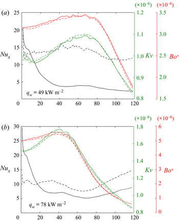
Figure 11 shows plots comparing and contrasting the non-dimensional factors of heat convection  ${ Nu}_x$ and thermal acceleration
 $Kv$ and buoyancy effect
 $Bo^*$ in all calculation cases. The
 $Bo^*$ and
 $Kv$ numbers are larger in the
 $78\ \textrm {kW}\ \textrm {m}^{-2}$ cases than in the
 $49\ \textrm {kW}\ \textrm {m}^{-2}$ cases. However, in both cases, the thermal acceleration non-dimensional factor
 $Kv$ is larger than
 $9.5\times 10^{-7}$, and the buoyancy non-dimensional factor
 $Bo^*$ is between
 $1.2\times 10^{-6}$ and
 $8.0\times 10^{-6}$, which means that the heat transfer is affected by the coupled effects of the thermal acceleration and buoyancy force. For upward flows, the two effects are both negative and contribute to heat transfer degradation. For downward flows, the buoyancy effect promotes heat transfer despite the existence of thermal acceleration effects.
Distributions of non-dimensional factors of heat convection  ${ Nu}_x$, thermal acceleration
 $Kv$ and the buoyancy effect
 $Bo^*$. Solid lines indicate upward flow. Dashed lines indicate downward flow.

3.1.2. Turbulence statistics
Figure 12 shows the radial profiles of the mean velocities in different cases. Significant flow acceleration in the streamwise direction occurs in both upward and downward cases. As can be seen in figures 12(a) and 12(b), for the cases with high flux, the shape of the radial profiles of the streamwise velocity  $u_x$ varies with flow direction. For the upward case, at first, the fluid near the wall speeds up substantially owing to a stronger buoyancy force, while the fluid near the pipe centre remains at a low speed, so that the velocity profile flattens at
 $x/d=10\text{--}20$ and then bends to be M-shaped; however, as the decrease in the cross-section average density takes effect later, the fluid near the pipe centre speeds up, and the velocity profile flattens again. For the downward case, the bulk velocity increases strongly during flow development. Because of the upward buoyancy force on the near-wall region, the fluid near the wall does not speed up over the main flow in the downward cases. For the lower heat flux cases in figure 12(c) and 12(d), the distortion of the velocity profiles is smaller. If the heat flux is not high enough, the effect of thermal acceleration might be overwhelmed by the buoyancy effect. It has been found that the thermal acceleration driven by an axial density gradient has a close relationship with the location and heat flux; unlike the buoyancy effect, which takes effect immediately very close to the inlet, the bulk density gradient needs time to develop. Therefore, the coupled effects of buoyancy and thermal acceleration contribute to a complicated multistage flow field.
Streamwise distributions of mean velocities for each simulation.

Both velocity fluctuations and mean profiles change. Figure 13 shows the root mean square of streamwise velocity fluctuations  $u_x''$ for Case A at different locations. The fluctuations decrease considerably at
 $x/d=10\text{--}20$, when the velocity profile becomes flat. While the velocity profile becomes M-shaped owing to the buoyancy effect at
 $x/d=40$, the flow fluctuations recover. Subsequently, another attenuation of the fluctuation takes place at
 $x/d=80$, followed by recovery again at
 $x/d=120$. This observation shows a consistent trend of development of the velocity profile. Large fluctuations mean drastic momentum exchange and thus efficient heat transfer within the fluid, which results in a higher convective heat transfer coefficient of the supercritical fluid. Note that the velocity distributions influence the turbulence intensities directly. When the radial gradient in the streamwise velocity
 ${\partial u_x}/{\partial r}$ decreases near the wall, the exchange between the low-speed flow at the near-wall region and the high-speed flow near the centre of the pipe is weakened, and the flow becomes steady and fluctuates less.
Root mean square of streamwise velocity fluctuations  $u''_x$ for Case A.

In the previous discussion, we pointed out that because of the coupled effects between the buoyancy force and thermal acceleration, the supercritical fluid in the pipe is accelerated both globally and locally and leads to different development periods of turbulent flow. To investigate the turbulence development, we write the budgets for the turbulent kinetic energy  $k=(\overline {\rho u_x''u_x''}+\overline {\rho u_r'' u_r''}+\overline {\rho u_\theta '' u_\theta ''})/2$. The buoyancy effects on the turbulence transport equation include two parts, the direct effect from the buoyancy production term
 $G_k$ and the indirect effects on the turbulence production term
 $P_k$.
The buoyancy production term  $G_k=\mp ({g R^*}/{U^{*2}_0})\overline {\rho 'u'_x}$ can be explained as the direct form of buoyancy effects on the turbulent kinetic energy, which influences the transport of turbulent kinetic energy in the flow direction in vertical flows. Note that negative and positive signs refer to upward and downward flows, respectively. Moreover, the buoyancy effects influence turbulence intensities indirectly through changing the signs and magnitudes of the streamwise velocity and Reynolds sheer stress in
 $-\overline {\rho u_x'' u_r''}({\partial \widetilde { u_x}}/{\partial r})$, which is the dominant term of turbulence production:
 $P_k=-\overline {\rho u_i'' u_j''}({\partial \widetilde { u_i}}/{\partial x_j})$. It is necessary to analyse the magnitudes of
 $G_k$ and
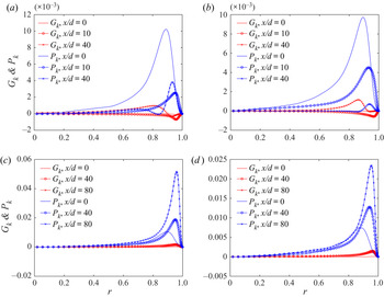
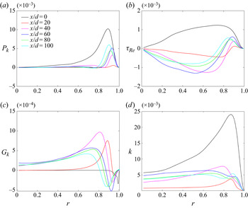
 $P_k$ in order to investigate the mechanism of turbulence development with buoyancy effects. Figure 14 shows the distribution of
 $G_k$ and
 $P_k$ for each simulation, respectively, at the same position. As we can see from figure 14(a) and 14(b), for upward flows in Case A and Case B, the buoyancy production
 $G_k= -({g R^*}/{U^{*2}_0})\overline {\rho 'u'_x}$ is neglected at the inlet and becomes negative at
 $x/d=10$. At the same time, the turbulence production
 $P_k=-\overline {\rho u_i'' u_j''}({\partial \widetilde { u_i}}/{\partial x_j})$ remains positive but decreases rapidly in magnitude. Different behaviour can be observed in these two cases at
 $x/d=40$. In Case A, there appears one positive peak as well as one negative peak of
 $G_k$ while two positive peaks of
 $P_k$. The first positive peak of
 $G_k$ and
 $P_k$ appears near to the centre of the tube, and contributes to the recovery of turbulent kinetic energy. The second positive peak of
 $P_k$ appears near the wall, corresponding to the negative peak of
 $G_k$. However, the positive magnitude of
 $P_k$ is larger than the negative magnitude of
 $G_k$, thus the whole production term is still positive at
 $x/d=40$. In Case B, both buoyancy production and turbulence production terms show one positive peak at
 $x/d=40$. In downward flow, different from the complicated behaviours in upward flow, both buoyancy production and turbulence production play a positive role in the whole flow field.
Buoyancy production terms  $G_k$ and turbulence production terms
 $P_k$ in the turbulent kinetic energy equation for each simulation: (a) for Case A, (b) for Case B, (c) for Case C and (d) for Case D.

Figure 15(a) and 15(b), respectively, show the distributions of the turbulence production term and the Reynolds shear stress of Case A during  $x/d=0\text{--}100$. Figure 15(d) shows the distribution of the buoyancy production term. Strong reductions in both
 $\overline {\rho u_x'' u_r''}$ and
 $P_k$ are observed. However, the development is not monotonic. Because the developing profile of the streamwise velocity is complicated, as shown in figure 12, the distributions of
 $\overline {\rho u_x'' u_r''}$ and
 $P_k$ exhibit a non-monotonic variation that can be described as ‘decrease–regenerate–decrease–regenerate’. Correspondingly, the turbulent kinetic energy
 $k$ decreases considerably at first, corresponding to strong turbulence suppression (figure 15c), and then recovers slightly. Although the buoyancy production term
 $G_k$ shows an opposite value to the turbulence production term
 $P_k$ in the buffer layer, its magnitude is much smaller. The combination of these two terms is still consistent with the effects of
 $P_k$. Therefore, the general behaviour of
 $k$ shown in figure 15(c) still follows the changes with
 $P_k$. In the section where the turbulent kinetic energy reaches the minimum, the flow is fully laminar, and a local wall temperature peak is observed nearby. Subsequently, as the fluid accelerates near the wall, the velocity profile becomes M-shaped, so that the velocity gradient reverses in the core region. This results in a negative Reynolds shear stress in the core and regeneration of turbulence production. Owing to the effect of thermal acceleration, the fluid in the centre of the pipe gradually catches up to the fluid near the wall and the velocity gradient decreases again. As a result, the Reynolds shear stress and turbulence intensities are suppressed again under global acceleration. Note that the appearance of
 $G_k>0$ in upward flows is closely related to the shape of the mean velocity profile (Bae et al. Reference Bae, Yoo and Choi2005), because of this the positive radial gradient of the streamwise velocity
 ${\partial \widetilde {u_x} }/{\partial r}$ is more likely to result in
 $-\overline {\rho ' u'_x}>0$ as long as the density gradient in the radial direction is negative. The positive
 $G_k$ term at
 $r<0.8$ mainly contributes to the supplements of turbulence in the core.
Reynolds shear stress, turbulence production and turbulence intensity distributions for Case A.

We define the combination production term  $\mathcal {P}_k$ as
 \begin{equation} \mathcal{P}_k = P_k + G_k ={-}\overline{\rho u_i'' u_j''}\dfrac{\partial \widetilde{ u_i}}{\partial x_j} \mp \dfrac{g R^*}{U^{*2}_0}\overline{\rho'u'_x}, \end{equation}
where the negative and positive signs refer to upward and downward flows, respectively, in the second term.
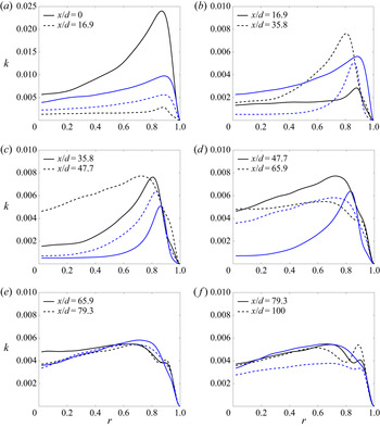
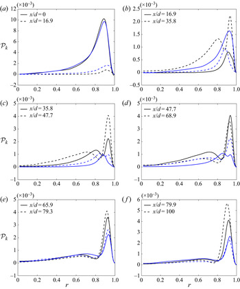
To investigate the acceleration of turbulence with respect to the heat fluxes, we compare the development of the turbulence intensities and production  $\mathcal {P}_k$ between the high heat flux and low heat flux cases (figures 16 and 17). As the Figures show, both cases exhibit a severe reduction in
 $\mathcal {P} _k$ and
 $k$ in the inlet section. This may be the consequence of the transition to the supercritical state. However, the attenuation period of Case A is shorter than that of Case B. A valid regeneration of turbulence can be observed at an early position during
 $x/d=16.9\text{--}47.7$ in Case A, but for the low heat flux case, the regeneration is long in coming at
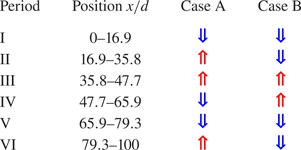
 $x/d=35.8$ in Case B. That is, the attenuation period can continue longer before the regeneration of the M-shaped velocity profile for the low heat flux case. After the recovery comes another attenuation owing to the global thermal acceleration, and the velocity profile becomes flatter again. Moreover, a second recovery occurs in Case A near the outlet, which is not observed in Case B. Table 3 provides a concise description of the developing periods of the turbulent kinetic energy in Cases A and B. It can be seen that under the coupled effects of buoyancy and thermal acceleration, the periodic heat transfer degradation phenomenon occurs as the fluid flows upwards. The higher the heat flux, the worse the turbulence attenuation; however, recovery occurs early in the high heat flux case because the competition between the buoyancy force and thermal acceleration is more fierce.
Distribution of turbulent intensities between reference Cases A and B. Black lines indicate Case A ( $q_w=78 \textrm {kW}\ \textrm {m}^{-2}$). Blue lines indicate Case B (
 $q_w=49 \textrm {kW}\ \textrm {m}^{-2}$).

Distribution of turbulence production between reference Cases A and B. Black lines indicate Case A ( $q_w=78 \ \textrm {kW}\ \textrm {m}^{-2}$). Blue lines indicate Case B (
 $q_w=49 \ \textrm {kW}\ \textrm {m}^{-2}$).

Summary of the developing periods of turbulent kinetic energy with respect to the flow acceleration under the effects of buoyancy force and thermal acceleration. Red arrow denotes enhancement of turbulence, blue arrow denotes attenuation of turbulence.

3.2. Heat transfer degradation mechanism
3.2.1. Energy conversion and equilibrium
One of the main advantages of DNS is the possibility of obtaining detailed information of the flow field, especially higher-order turbulence statistics. To investigate the energy conversion and equilibrium of the supercritical fluid, we write the Favre-averaged energy equation of turbulent kinetic energy  $k=(\overline {\rho u_i'' u_i''})/2$ and mean kinetic energy
 $K=(\bar {\rho } \widetilde {u_i}\widetilde {u_i})/2$.
The Favre-averaged turbulent kinetic energy equation is given by
 \begin{align} \dfrac{\partial k}{\partial t}+\widetilde{u_j}\dfrac{\partial k}{\partial x_j} & =P_k-\bar{\rho}\varepsilon -\overline{u_i''}\dfrac{\partial \bar{p}}{\partial x_i}+\overline{u_i''}\dfrac{\partial \overline{t}_{ij}}{\partial x_j}+\overline{p'\dfrac{\partial u_i''}{\partial x_i}} \nonumber\\ & \quad + \dfrac{\partial}{\partial x_j}\left[\overline{t_{ij}'u_i''}-\dfrac{1}{2}\overline{\rho u_j''u_i''u_i''}-\overline{p'u_j''}\right]. \end{align}
The Favre-averaged mean kinetic energy equation is given by
 \begin{equation} \frac{\partial K}{\partial t}+\widetilde{u_j}\frac{\partial K}{\partial x_j}=\frac{\partial}{\partial x_j}\left(\dfrac{1}{2} \bar{\mu} \dfrac{\partial \widetilde{u_i} \widetilde{u_i}}{\partial x_j}-\bar{p} \widetilde{u_i}+\tau_{ij}\widetilde{u_i}\right)-P_k-\bar{\mu}\left(\dfrac{\partial \widetilde{u_i}}{\partial x_j}\right)^2, \end{equation}
where:
(i) the Reynolds shear stress
(3.18)\begin{equation} \tau_{ij}={-}\overline{\rho u_i''u_j''};\end{equation}(ii) the production of turbulent kinetic energy
(3.19)\begin{equation} P_k=\tau_{ij}\frac{\partial \widetilde{u_i}}{\partial x_j};\end{equation}(iii) viscous shear stress
(3.20)$$\begin{gather} t_{ij}=2\frac{\mu}{Re_0}\left(S_{ij}-\frac{1}{3} \frac{\partial \widetilde{u_k}}{\partial x_k}\delta_{ij}\right), \end{gather}$$(3.21)$$\begin{gather}S_{ij}=\frac{1}{2}\left(\dfrac{\partial \widetilde{u_i}}{\partial x_j}+\dfrac{\partial \widetilde{u_j}}{\partial x_i}\right); \end{gather}$$(iv) dissipation rate
(3.22)\begin{equation} \bar{\rho} \varepsilon =\overline{t_{ij}'\frac{\partial u_i''}{\partial x_j}}. \end{equation}


Comparing the mean energy as described in (3.17) with the turbulent kinetic energy as described in (3.16), we see that indeed the opposite term of  $-P_k=-\tau _{ij}({\partial \widetilde {u_i}}/{\partial x_j})$ on the right-hand side of the mean-energy equation is the production term of turbulent kinetic energy. The energy conversion from the mean flow to the turbulent flow provides the maintenance mechanism of turbulent energy. The developing profiles of the streamwise velocity influence the turbulence intensities by impeding the energy conversion from the mean flow kinetic energy to the turbulent kinetic energy by
 $P_k$, and therefore the mean kinetic energy increases considerably under acceleration, while the turbulence intensity is instead constrained.
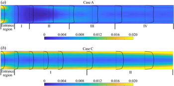
Turbulence attenuation is closely related to the convective heat transfer coefficient. However, in supercritical flow under the coupled effects of buoyancy and thermal acceleration, there are four distinct periods. Figure 18 shows the developing periods of turbulent flow and heat transfer. During these periods, the emergence and attenuation of turbulent kinetic energy corresponds to the coupled effects. For upward flow (see figure 18a), in addition to the entrance region, the positive effect and negative effect alternate over four periods of the turbulent heat transfer. Period I  $x/d=10\text{--}16.9$ is the period of suppression with significant heat transfer degradation and turbulence attenuation. During period II
 $x/d=16.9\text{--}47.7$, heat transfer recovers. Next, during period III from
 $x/d=47.7$ to
 $x/d=79.3$, heat transfer degrades again. Subsequently, a recovery occurs again in period IV
 $x/d=79.3\text{--}120$. For downward flow (see figure 18b), heat transfer is enhanced in period I because the buoyancy force opposite to the flow direction increases the near-wall shear stress. In period II, the efficacy of the heat transfer begin to reduce as the fluid gradually enters the supercritical state. Then, the flow acceleration, driven by the density gradient of the bulk flow, increases the flow Reynolds number significantly.
The development of the turbulent kinetic energy and the streamwise velocity for Cases A and C. Lines represent the radial profile of streamwise velocity. Contours represent the distribution of the turbulent kinetic energy.

To illustrate the coupled buoyancy and thermal acceleration effects on the specific periods, intuitive quantification criteria are proposed to measure their effects. We define a regional acceleration coefficient  $AC_{area}$ to measure the streamwise flow acceleration level in the cross-section. To measure the flow acceleration in region
 $A< y^+< B$, the regional acceleration coefficient is written as
 \begin{equation} Ac_{area}=\frac{\partial}{\partial x}\left(\frac{\int_{r_A}^{r_B}\int_{0}^{2{\rm \pi}}\widetilde{u_x}r\,\textrm{d}\theta \,\textrm{d}r}{\int_{r_A}^{r_B}\int_{0}^{2{\rm \pi}}r \,\textrm{d}\theta \,\textrm{d}r}\right) \end{equation}
in which  $r_A$ is the radial coordinate, where
 $y^+=A$,
 $r_B$ is the radial coordinate, where
 $y^+=B$ and the non-dimensional wall distance
 $y^+={r u_\tau }/{\nu }$.
Based on this, we define  $Ac_{bulk}$ and
 $Ac_{near\text {-}wall}$ as
 \begin{gather} Ac_{bulk}=\frac{\partial}{\partial x} \left(\frac{ \int_0^{r_1} \int_0^{2{\rm \pi}}\widetilde{u_x} r \,\textrm{d}\theta \,\textrm{d}r }{\int_0^{r_1} \int_0^{2{\rm \pi}}r \,\textrm{d}\theta \,\textrm{d}r} \right), \end{gather}
 \begin{gather} Ac_{near\text{-}wall}=\frac{\partial }{\partial x}\left(\frac{\int_{r_2}^{r_3}\int_{0}^{2{\rm \pi}}\widetilde{u_x} r \,\textrm{d}\theta \,\textrm{d}r}{\int_{r_2}^{r_3}\int_0^{2{\rm \pi}} r \,\textrm{d}\theta \,\textrm{d}r} \right) \end{gather}
in which  $r_1$ is the radial coordinate where
 $y^+=100$,
 $r_2$ is the radial coordinate where
 $y^+=35$ and
 $r_3$ is the radial coordinate where
 $y^+=40$. In this paper, the centre region of the flow is set to be
 $y^+>100$. Therefore, we choose
 $Ac_{bulk}$ to measure the global effect of the thermal acceleration in the centre region. The significant departures from fully turbulent flow caused by temporal acceleration are evident at
 $y^+<50$ only and the non-dimensional velocity gradient reaches the local minimum at
 $y^+\approx 50$ (Peeters et al. Reference Peeters, Pecnik, Rohde, Van Der Hagen and Boersma2016). Therefore,
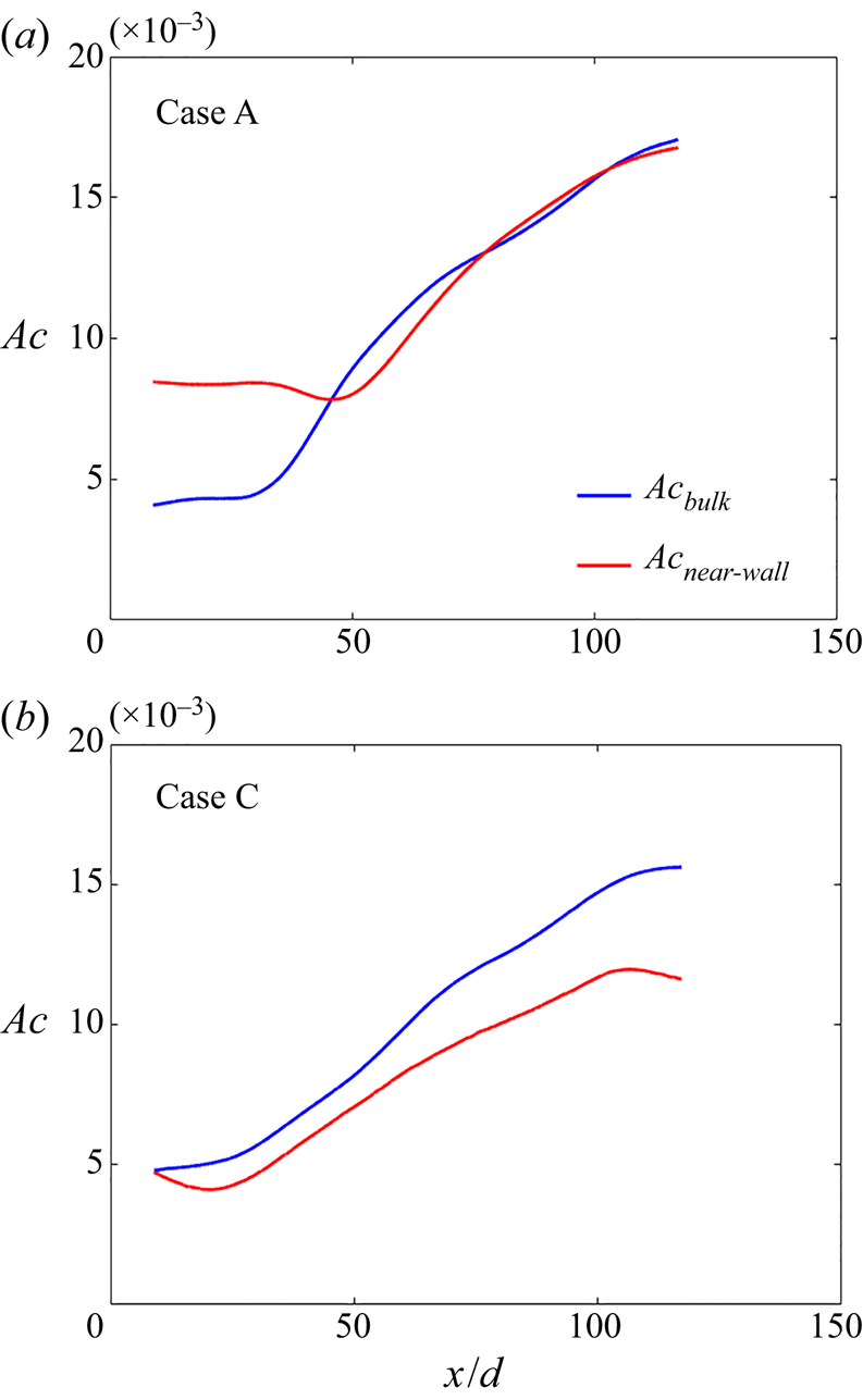
 $Ac_{near\text {-}wall}$ is calculated to measure the local acceleration caused by the buoyancy force in the near-wall region. We calculate the acceleration coefficients with DNS time-averaged data and smooth the data by filtering with a Gaussian window. Figure 19 shows the smoothed data and the distribution of
 $Ac_{bulk}$ and
 $Ac_{near\text {-}wall}$ for Case A (upward case) and Case C (downward case). According to figure 19(a),
 $Ac_{near\text {-}wall}$ is larger than
 $Ac_{bulk}$ for
 $x/d=0\text{--}40$ in Case A, which means that buoyancy can take effect at the very early location and is the dominant factor of the first two periods in figure 18(a). In period I, the buoyancy force contributes to the heat transfer degradation directly by flattening the streamwise velocity profiles. Subsequently, the heat transfer recovers to some degree by regenerating the turbulence intensities in period II because of the M-shaped velocity profiles. The global flow acceleration driven by the axial gradient of bulk density begins to emerge in period III and causes the heat transfer to deteriorate again. This is because the bulk density gradient needs time to develop, the thermal acceleration effect takes place later after the buoyancy effect. Subsequently, as more fluid transitions to the supercritical state, the bulk density gradient is no longer significant; the buoyancy dominates again in the last period. Under these conditions, heat transfer recovers.
Distribution of  $Ac_{bulk}$ and
 $Ac_{near\text {-}wall}$ for Cases A and C.

In Case C,  $Ac_{bulk}$ and
 $Ac_{near\text {-}wall}$ both increase in the flow direction. However, as the upward flows are the same, the effect of thermal acceleration in the downward flow is ultimately the product of the axial gradient of the bulk density; that is, it cannot eliminate certain temporal limitations. The buoyancy dominates at first, local deceleration in the near-wall region enhance the turbulence strength. In period II, the fluid transform to supercritical state, leading to short-term heat transfer degradation. Finally, thermal acceleration takes effect, promotes turbulence and enhances heat transfer by increasing the Reynolds number
 $Re_b$ and the Reynolds shear stress
 $\tau _{Re}$.
Combining the acceleration coefficients with the analysis already described, we define a  $Ba^*$ number to evaluate the coupling effects of buoyancy and thermal acceleration on the turbulent heat transfer at SCP. Here,
 ${{\partial \widetilde {u_x}}/{\partial r} } |_{\lambda _1}$ and
 ${{\partial \widetilde {u_x}}/{\partial r}}|_{\lambda _2}$ represent the averaged radial gradient of the streamwise velocity for
 $\lambda _1:40< y^+<50$ and
 $\lambda _2:10< y^+<20$, respectively, which describe the shape of the velocity distribution of the buffer layer. The
 $Ba^*$ number denotes the effect as well as the location of the heat transfer degradation and enhancement caused by the coupling effects. The signature of
 $Ba^*$ indicates that the coupling effects are negative or positive, the absolute value of
 $Ba^*$ indicates the degree of the deterioration or enhancement. For example, if
 $Ba^*>0$, it means that the turbulence is regenerated or enhanced owing to the effects of buoyancy and thermal acceleration. The distributions of the
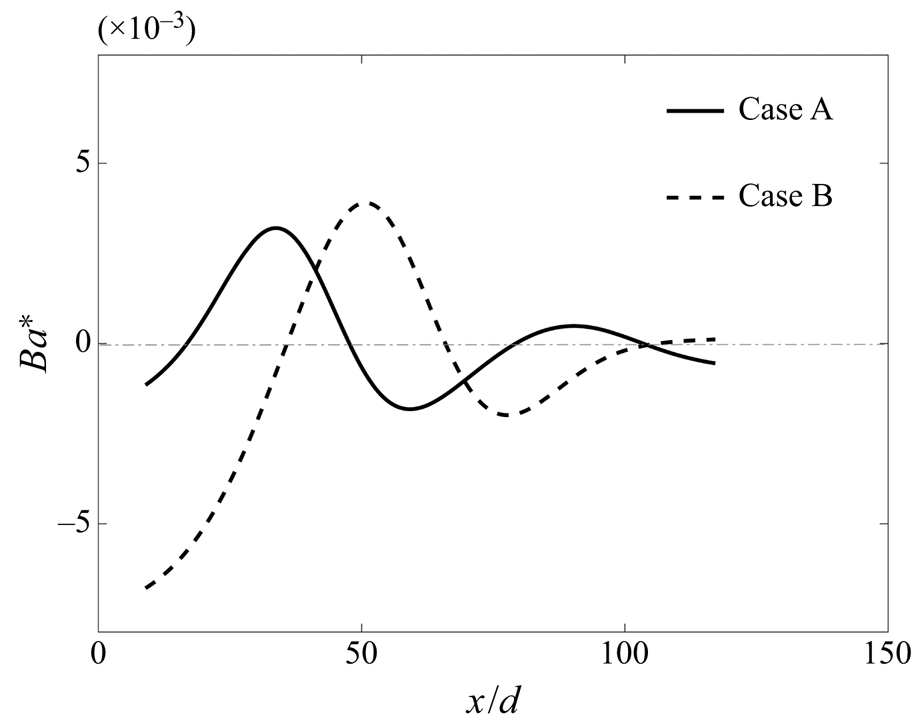
 $Ba^*$ number for Cases A and B are shown in figure 20. The attenuation occurs earlier in Case A than in Case B. The heat transfer degradation and recovery are consistent with the heat transfer periods proposed in the previous discussion. This provides an explanation for the complicated heat transfer phenomenon, with both temperature distribution peaks and valleys, under the coupled effects of buoyancy and thermal acceleration.
 \begin{equation} Ba^*=(Ac_{bulk} -Ac_{near\text{-}wall})*\left(\left.\frac{\partial \widetilde{u_x}}{\partial r}\right|_{\lambda_1}*\left. \frac{\partial \widetilde{u_x}}{\partial r}\right|_{\lambda_2}\right). \end{equation}
Local buoyancy and thermal acceleration effect number  $Ba^*$ distributions along the vertical tube for Cases A and B.

3.2.2. The effects of buoyancy and thermal acceleration on the turbulent structures
In the previous section we discussed how the coupled interaction of buoyancy and thermal acceleration contributed to the developing periods of turbulence intensities and heat transfer by changing the turbulence production, but we did not show how the turbulent structures are affected. As these structures are significant to the self-regenerating process of the near-wall turbulence and the spanwise heat transfer behaviour, an investigation of how the coupled effects of buoyancy and thermal acceleration disturb the streamwise vortices and the near-wall streaks is necessary. Peeters et al. (Reference Peeters, Pecnik, Rohde, Van Der Hagen and Boersma2016)'s work showed that variable thermophysical property fluctuations can influence the formation of turbulent structures. We investigate here how streamwise vortices and near-wall streaks develop under strong flow acceleration in the streamwise direction.
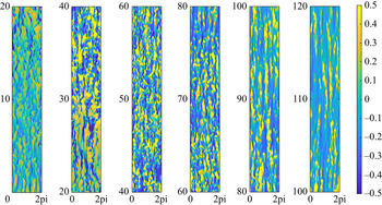
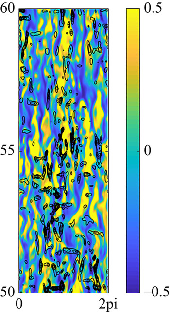
To describe the near-wall streaks with density variations, we use  $(\rho u_x)'=\rho u_x - \overline {\rho u_x}$ to show the magnitude of the streaks. Figure 21 shows the distribution of the streaks at
 $y^+=20$ in the streamwise direction in Case A. The streaks become regular and wide under the buoyancy forces in the first period
 $x/d=10\text{--}20$; then, the magnitude of the streak increases in period II
 $x/d=20\text{--}40$, but the streaks decrease again and show laminar characteristics as the thermal acceleration begins to predominate. The ejections and sweeps of the streaks are also reduced as the strength decreases, which is largely responsible for the velocity fluctuations. Therefore, it is clear that the streak magnitude is consistent with the turbulent motions as discussed in § 3.1.2.
Instantaneous isosurfaces of the streaks  $(\rho u_x)'$ at
 $y^+=20$ in Case A.

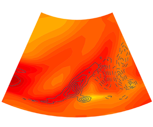
To investigate the mechanism of how the streaks are disrupted under the flow acceleration, we plot the contours of  ${\partial u_x}/{\partial x}$ and the streaks
 $(\rho u_x)'$ in one picture (figure 22). In the region where the streaks are damaged, the speed-up area is exactly coincident with the low-speed streaks. Under these conditions, the difference between the low-speed streaks and the high-speed streaks is reduced. Thus, the flow is stabilised and laminarised with less fluctuation and fewer steaks.
Contour plots of streaks at  $y^+=20$ in Case A. The black lines indicate isolines of
 ${\partial u_x}/{\partial x}>0$.

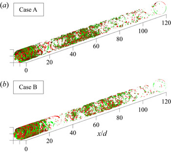
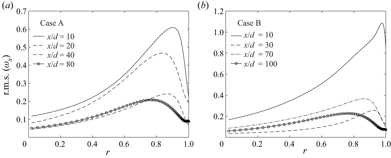
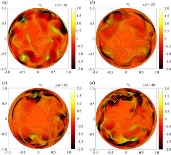
To investigate turbulent structures in the variable-density flow, we define the vorticity as  $\boldsymbol {\omega }=\boldsymbol {\nabla }\times (\rho \boldsymbol {u})$ to take density into consideration. Figures 23 and 24 provide the distributions of instantaneous isosurfaces and root mean square of the streamwise vortices
 $\omega _x=({1}/{r})({\partial (r\rho u_{\theta })}/{\partial r}-{\partial (\rho u_r)}/{\partial \theta })$ in the pipe. Isosurfaces of
 $\omega _x=\pm 1.0$ are shown in red and green, respectively, viewing from the radial direction. The turbulent laminarisation is revealed by the reduction in the strength of vorticity motions. For the fully laminar regions such as the outlet of Case A with
 $x/d=20$ and Case B with
 $x/d=30$, the vorticity motions become so weak that the isosurfaces are sparse. According to figures 7 and 23, during the heat transfer degradation section, the streamwise vortices are reduced, and the sweep and ejection events are decreased greatly. During the heat transfer recovery section, the streamwise vortices can be regenerated to some degree. The decrease in streamwise vorticity in the pipe suggests diminished wall-normal and circumferential motion. In contrast, an increase in streamwise vorticity suggests enhanced wall-normal and circumferential motion. The more vigorous the wall-normal and circumferential motion, the stronger the heat transfer between the wall and the flow. For upward flow, the higher heat fluxes in Case A show early and abbreviated attenuation and then immediate regeneration. The streamwise vorticity substantially decreases as a result of the buoyancy force at the early location
 $x/d=10\text{--}20$ and increases after the M-shaped velocity profile appears. In Case B, as the heat flux is lower, the buoyancy and thermal acceleration slowly increases as the flow move downstream, so the decrease and increase in the streamwise vortices appear later and last longer.
Instantaneous isosurfaces of the streamwise vorticity for upward flows from bottom to top for Cases A and B.

Root mean square of the streamwise vorticity at different locations for upward flows for Cases A and B.

Taking the curl of the momentum equation, we can obtain the evolution equation of the momentum vorticity:
 $$\begin{gather} \frac{\partial \boldsymbol{\omega}}{\partial t} + \underbrace{\boldsymbol{u}\boldsymbol{\cdot}\boldsymbol{\nabla}\boldsymbol{\omega}}_{convection}=\underbrace{\omega\boldsymbol{\cdot} \boldsymbol{\nabla} \boldsymbol{u}}_{production} + \underbrace{\frac{1}{Re_0}\boldsymbol{\nabla}\boldsymbol{\cdot}\mu \boldsymbol{\nabla} (\boldsymbol{\nabla} \times \boldsymbol{u})}_{diffusion\ and\ dissipation} + \underbrace{\frac{1}{Fr}\boldsymbol{\nabla} \times \rho \boldsymbol{x}}_{buoyancy} - \underbrace{\boldsymbol{\nabla} \times \psi \rho \boldsymbol{u}}_{thermal\ expansion} \nonumber\\ - \underbrace{\boldsymbol{\nabla} \times K \boldsymbol{\nabla} \rho}_{torque} + \underbrace{Re_0 \boldsymbol{\nabla} \cdot (2\boldsymbol{\nabla} \mu \times \boldsymbol{S})}_{viscosity\ gradient}, \end{gather}$$
where  $\varPsi =\boldsymbol {\nabla }\boldsymbol {\cdot } \boldsymbol {u}$,
 $K=(\boldsymbol {u} \cdot \boldsymbol {u})/2$, and
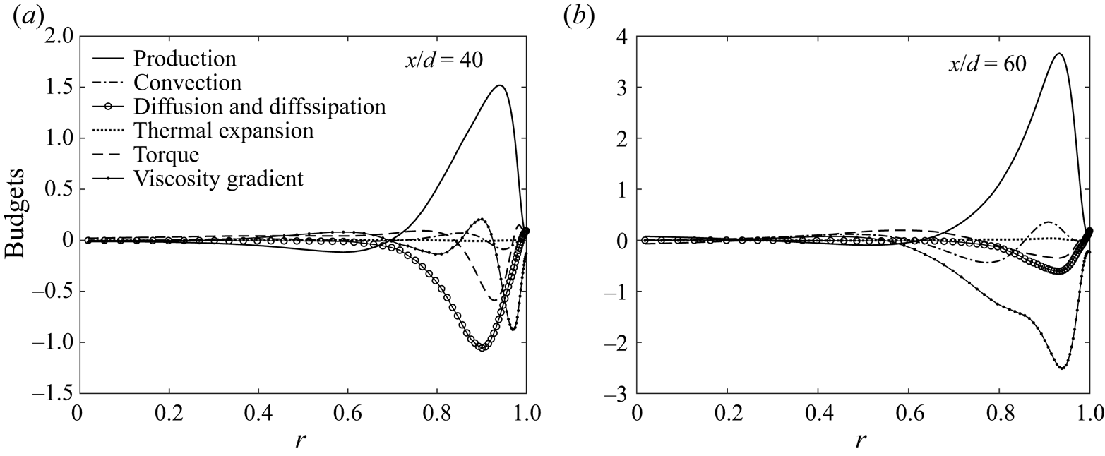
 $\boldsymbol {S}$ is the deviatoric stress tensor. The first term on the right-hand side represents the production of the momentum vorticity, and the deformation rate directly affects the vorticity. The second term on the right-hand side represents diffusion and dissipation, which transports the vorticity from the high-vorticity area to the low-vorticity area. The other terms represent the effects of buoyancy, thermal expansion, torque and viscosity gradients. Figure 25 shows the budgets of the streamwise vortices
 $\omega _x=({1}/{r})({\partial (r\rho u_{\theta })}/{\partial r}-{\partial (\rho u_r)}/{\partial \theta })$, in (3.27). The buoyancy term
 $(({1}/{Fr})\boldsymbol {\nabla } \times \rho \boldsymbol {x})_x$ is equivalent to zero in the vertical direction. The thermal expansion term is small too in the whole radial region. Therefore, the direct influence of both buoyancy and thermal expansion effects on the streamwise vortices can be neglected. As we can see from the figure, the production and convection terms are the main sources of the streamwise vortices, while the diffusion, dissipation term and torque terms are the main sink terms. The viscosity gradient term, however, has a significant negative influence while the M-shaped velocity profile is manifest. The production term is much larger at
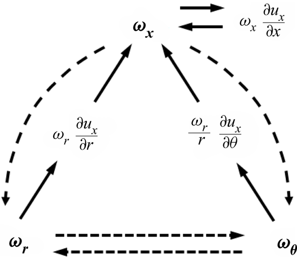
 $x/d=60$, which corresponds with the instantaneous streamwise vorticity distribution in figure 23(b). To evaluate the production of the streamwise vorticity, we write the component of the production term in (3.27):
 \begin{equation} \underbrace{\omega_x \dfrac{\partial u_x}{\partial x}}_{stretching}+\underbrace{\omega_r \dfrac{\partial u_x}{\partial r}+\dfrac{\omega_\theta}{r}\dfrac{\partial u_x}{\partial \theta}}_{tilting}. \end{equation}
Budgets of the streamwise vortices  $\omega _x=({1}/{r})({\partial (r\rho u_{\theta })}/{\partial r}-{\partial (\rho u_r)}/{\partial \theta })$ at different positions for upward flow Case B: (a)
 $x/d=40$; (b)
 $x/d=60$.

The production of the streamwise momentum vorticity consists of three terms: the first term is a stretching term, and the second and third terms are tilting terms. As shown in figure 26, the streamwise momentum vorticity  $\omega _x$ starts from the tilting effects between
 $\omega _r$ and the radial gradient of the streamwise velocity in the near-wall region, as the circumferential gradient of the velocity is almost zero. The stretching effect makes the vortices elongate
 $(\omega _x ({\partial u_x}/{\partial x})>0)$ or contract
 $(\omega _x ({\partial u_x}/{\partial x})<0)$; thus, streamwise acceleration increases the vortex strength, and streamwise deceleration decreases the vortex strength. However, turbulent pipe flow is an anisotropic three-dimensional phenomenon, so the streamwise vorticity is related to the vorticity in the other two directions. Under the effect of thermal acceleration and buoyancy, the stretching function is incongruously enhanced, while the tilting function is reduced. The significant stretching function destroys the balance of the three-dimensional vortices, and the streamwise vortices gradually stretch to the point of dissipation (figure 27).
The generative mechanism of the streamwise momentum vorticity.

Instantaneous isosurfaces of the streamwise momentum vorticity  $\omega _x$ in Case A.

Fu, Li & Wang (Reference Fu, Li and Wang2003) introduced a new parameter  $\eta _4$ for identifying the vortex stretching mechanism. The parameter
 $\eta _4$ in the streamwise momentum vorticity
 $\omega _x$ is
 \begin{equation} \eta_4=S_{11}W_{23}^2=0.25\omega_x^2\dfrac{\partial u_x}{\partial x}. \end{equation}
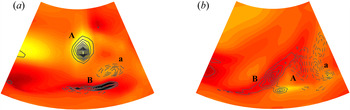
The vortex therefore stretches (relaxes) when the flow is accelerating (decelerating), i.e.  $(\eta _4<0)$. Figure 28 shows the contours of both streamwise momentum vorticity and
 $\eta _4$ of two close positions
 $x/d=16.6$ and
 $x/d=16.9$ in the streamwise direction. Here, the large-scale vorticity structures can be clearly observed. The generative mechanism of the streamwise momentum vorticity can be further clarified with the contour lines of
 $\eta _4$. In figure 28(a), two obvious acceleration regions
 $(\eta _4>0)$ are shown exactly at the positions of the streamwise momentum vorticity A and B, and a deceleration region locates with the streamwise momentum vorticity A. It is clear that after the acceleration, vorticity A breaks and diffuses with local deceleration area, vorticity B breaks and decelerates, then the intensity of vorticity decreases considerably at
 $x/d=16.9$. The result is that under buoyancy-driven local flow acceleration, the stretching term acts as a sink term for the formation of streamwise momentum vorticity. In this period, the ejections and sweeps in the near-wall region are also suppressed, which shows that the generation of streamwise vortices owing to the ejections and sweeps decrease.
Contours of streamwise momentum vorticity  $\omega _x$ and contour lines of
 $\eta _4$ in Case A: (a)
 $x/d=16.6$; (b)
 $x/d=16.9$. Positive contours
 $\eta _4>0$ are shown as solid lines. Negative contours
 $\eta _4<0$ are dashed.

4. Conclusion
In this paper, we have investigated the mechanism of heat transfer for supercritical  $\textrm {CO}_2$ flowing in a heated vertical tube with coupling effects of buoyancy and thermal acceleration by means of DNS. There is good agreement between the DNS results and the experimental data. The simulation predicts a complicated heat transfer law under the coupling influence, including a local heat transfer degradation and recovery. The higher the heat fluxes, the more sharply the peak wall temperature increases. However, in downward flows, no significant increase in the wall temperature or peaks are observed.
The non-uniform temperature distribution leads to a non-uniform thermophysical property distribution in the cross-section as well as in the streamwise direction. Large density and viscosity variations are found near the inner wall in both radial and axial directions. Owing to this, the turbulent flow operates under the coupled effects of buoyancy and thermal acceleration, which trigger a series of perturbations on turbulence development.
The competition between the buoyancy and thermal acceleration leads to the development of profiles of streamwise velocity, which influence the turbulence intensities by impeding the energy conversion from the mean flow kinetic energy to the turbulent kinetic energy by  $P_k$; therefore, the mean kinetic energy increases considerably under acceleration, while the turbulence intensity is instead constrained.
The attenuation and regeneration of turbulence are closely related to the heat transfer performance. However, for heat transfer with buoyancy and thermal acceleration cases, there are four distinct periods. For upward flows, the buoyancy can take effect immediately at a very early location and is the dominant factor of the first two periods. Because the bulk density gradient needs time to develop, the thermal acceleration takes effect later, after the buoyancy effect. Subsequently, as the fluid transitions to the supercritical state, the bulk density gradient is no longer important, so the buoyancy predominates again in the last period. An acceleration coefficient is proposed and used to determine the  $Ba^*$ number to evaluate the effects of buoyancy and thermal acceleration on the turbulent heat transfer. The parameters
 $Ac_{bulk}$ and
 $Ac_{near\text {-}wall}$ provide an effective way to distinguish the dominant factor of heat transfer at different periods. Furthermore, the
 $Ba^*$ number defines an accurate criterion for heat transfer degradation under the complex coupling effects of buoyancy and thermal acceleration.
The generative mechanism of turbulent structures under the effects of buoyancy and thermal acceleration was analysed. In the acceleration region, the streaks become regular and wide. This is because the speed-up area is coincident with the low-speed streaks, reducing the difference between the streaks, which decrease the sweep and ejection events in the near-wall region and hinder turbulence regeneration. For the streamwise vortices, during the heat transfer degradation section, the streamwise vortices are reduced. The significant flow acceleration is anisotropically three-dimensional and stretches the vortices to their ultimate destruction.
Funding
This project was supported by the National Natural Science Foundation of China (no. 51536004) and the Science Fund for Creative Research Groups of China (no. 51621062).
Declaration of interests
The authors report no conflict of interest.