1. Introduction
The goal of natural language processing (NLP) is to analyse and understand text data automatically. Negation detection is a subproblem within NLP that consists of identifying negation cues and their scopes. For our objectives, we treat negation detection as assertion of whether the entity in question is present or absent, where ambiguous cases are treated as absent. Entities are key terms, such as disease names, and location or time modifiers of those diseases. For example, in the excerpt ‘there was no tumour present. The same is true for atrophy but there is evidence of an acute ischaemic stroke’, both tumour and atrophy are negated and ischaemic stroke is not. Acute is a time modifier and is also not negated as it refers to the non-negated ischaemic stroke.
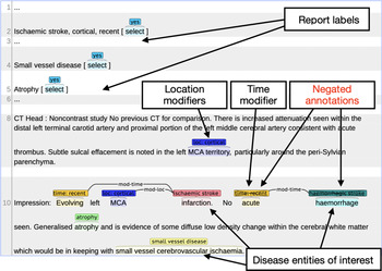
We apply negation detection to the analysis of radiology reports, written natural language text describing findings and observations of medical health professionals. We used the Edinburgh Stroke Study (ESS) and the National Health Service Tayside (Tayside) datasets, which both consist of reports of radiology scans of the brain. Our entities on which we do negation detection are names of diseases, the anatomical location of the disease, and whether development of the disease is recent or old. Due to the sensitivity of the data, we provide a realistic synthetic example of a radiology report in Figure 1, where negated entity annotations are crossed out.
An example of a synthetic yet realistic brain imaging report with disease entity, modifier, negation, relation and label annotations created for the ESS and Tayside datasets. Manual annotation used for development, training and evaluation were conducted using the brat annotation tool (Stenetorp et al. Reference Stenetorp, Pyysalo, Topić, Ohta, Ananiadou and Tsujii2012).

The work presented here is part of an MRC Mental Health Data Pathfinder project on linking data extracted from brain imaging reports to EHR data on mental health with the aim to study correlations between physical and mental health in the Generation Scotland cohort.Footnote a One aim of the NLP work in this Pathfinder project is to label radiology reports with an indication of what was observed by the radiologist, such as disease type, location of the disease and whether the disease is recent or old. This is a text mining task involving named entity recognition (NER), negation detection, relation extraction and document classification. We are developing a rule-based system called EdIE-R (Edinburgh Information Extraction for Radiology Reports) containing these four processing components (Alex et al. Reference Alex, Grover, Tobin, Sudlow, Mair and Whiteley2019). We are also experimenting with machine learning alternatives for each component making use of neural networks. We have previously presented a method comparison for the NER step (Gorinski et al. Reference Gorinski, Wu, Grover, Tobin, Talbot, Whalley, Sudlow, Whiteley and Alex2019) and showed that it is difficult to outperform a rule-based system specifically designed for recognising named entities in brain imaging reports.
In this paper, we focus on the negation detection step. We assume that the disease entity and modifier spans are known and compare each model’s ability to predict on the unseen test sets whether these disease entity and modifiers are negated or not. We also provide an analysis of negation in our data. We compare three rule-based methods and two based on neural networks:
pyConText, a rule-based negation detection tool which is available as a Python implementation of ConText, a variation of the widely used NegEx algorithm (see Section 5.1),
NegBio, a rule-based tool for negation and uncertainty detection in clinical texts (see Section 5.1),
EdIE-R-Neg, a rule-based negation detection component in EdIE-R which was specifically developed for analysing brain imaging reports (see Section 5.2),
FFNN-Neg, a feedforward neural network trained on brain imaging reports for negation detection (see Section 5.4), and
BiLSTM-Neg, a bidirectional recurrent neural network (RNN) trained on brain imaging reports for negation detection (see Section 5.5).
For each approach, we report overall negation detection results and provide analysis where performance varied by entity type and subtype.
Our models are developed, trained and tested on two datasets of radiology reports from the ESS (
 $n=630$
) (Jackson et al. Reference Jackson, Crossland, Dennis, Wardlaw and Sudlow2008) and NHS Tayside (Tayside,
 $n=1062$
). These were manually annotated for 12 named entity types and 4 modifiers. Training and development was largely done on the development subset of the ESS dataset, and evaluation was carried out on unseen test subsets of both.
To test generalisation and the effectiveness of porting our models to similar datasets, we ran cross-training experiments on the machine learning models, evaluating whether introduction of parts of the Tayside development data into the training set (transfer learning, see Pratt, Mostow and Kamm Reference Pratt, Mostow and Kamm1991), increased performance on the Tayside test set.
The experiments described in this paper are preceded by a corpus analysis to illustrate the nature of negation cues in such data. From the corpus analysis, we discover that the negation detection task as we frame it is relatively straightforward, due to factors such as not needing to identify scope and treating uncertain cases as negative. In addition, negation patterns in radiology reports are known to be more simple than in other documents. We treat negation as a binary classification or assertion of definite presence of medical entities (presence vs. non-presence), as is often done in clinical NLP. This application is different to how negation is generally conceptualised in linguistics literature. It was chosen due to the wider project aims of document classification and labelling radiology reports with an indication of what was observed by the radiologist, for which binary classification is more useful than other approaches that focus on identifying scope or ambiguous cases. That this conceptualisation makes the task less complex is evidenced by the high F1 scores of our models.
2. Motivation for using neural networks for negation detection
Rule-based NLP models are often employed for information extraction and labelling of raw text documents, particularly in the medical field where labelled training data are often sparse or non-existent (e.g., see examples in Pons et al. Reference Pons, Braun, Hunink and Kors2016). As we initially had no annotated data available for the purpose of text mining brain imaging reports, the rule-based EdIE-R system was developed as a starting point. In parallel with writing rules for EdIE-R, data from the ESS and NHS Tayside were annotated manually by domain experts to create gold standard data for evaluation.
The annotated datasets, which we now have available and are used for the experiments presented here, amount to over 1600 reports containing over 13,000 entity annotations in total. This means that the use of machine learning, and in particular neural networks, becomes more viable. Rule-based systems, while highly effective, are time-consuming to set up and can sometimes translate poorly between datasets. In this paper, we show that an effective neural network can give near-equivalent performance when used for negation detection. Once an effective neural network model has been found, we would expect it to have the benefit of being quicker to adapt to new datasets that differ more greatly than the two analysed here, as hyperparameters and architecture should translate reasonably between datasets meaning only fine-tuning is necessary.
In addition to the rule-based model, we have therefore developed neural network models which learn to detect negation by capturing negation patterns in the annotated data. In both cases, we treat negation detection as binary classification limiting our predictions to entity tokens, the spans of which we assume are already known. Here we test two neural network architectures, a feedforward neural network (FFNN) and a bidirectional long short-term memory (BiLSTM) neural network.
Similar to previous work (Fancellu, Lopez, and Webber Reference Fancellu, Lopez and Webber2016), we begin our investigation using a feedforward network as a baseline neural network model. Apart from being a simpler and faster model to train than BiLSTMs, using a feedforward network is appealing as controlling the amount of surrounding context used to predict negation is achieved easily. While BiLSTMs are more powerful models that can learn what salient information to store in their internal state, we assume they may need more data to do so. Therefore, truncating the input for use with a feedforward network may be beneficial in a low-resource setting. In their related work on negation scope detection, Fancellu et al. (Reference Fancellu, Lopez and Webber2016) used window sizes of 9 and 15 tokens, as for their English literature datasets, it was found that 95% of words in the negation scope occurred within a window of 9 tokens to the left and 15 to the right of the negation cue. As we shall see in Section 4.1, in the ESS radiology report dataset, the context window containing the negation cues most useful for negation detection is skewed to the left but also has tails that taper off at similar distances from the negated token, 15 tokens to the left and 10 to the right.
LSTMs (Hochreiter and Schmidhuber Reference Hochreiter and Schmidhuber1997), the second type of neural network approach evaluated here, are recurrent neural networks (RNNs). RNNs are often employed in NLP tasks due to their effectiveness at modelling sequences of arbitrary length. This makes them in theory able to take advantage of long-distance dependencies in the input, which would be impossible to capture with any finite window feedforward or convolutional neural network. However, traditional RNNs were demonstrated to suffer from exploding/vanishing gradients (Bengio et al. Reference Bengio, Simard and Frasconi1994), an issue that impedes learning and limits the effective maximum distance of dependencies that can be learned in practice.
LSTMs are an augmented RNN architecture that ameliorates the exploding/vanishing gradients issue through use of an internal gating system. The gating system controls the flow of information to and from the hidden state/memory of the network, demonstrably improving its ability to capture distant dependencies. BiLSTMs (Graves and Schmidhuber Reference Graves and Schmidhuber2005) are a further extension to the LSTM model that take into account both the left and the right context of an input when constructing its representation. This property is very important for negation detection, as negation cues can precede or succeed a target word in our dataset, as we will show when analysing negation cue patterns in Section 4.1.
3. Related work
A popular approach for negation detection is the use of regular expressions, such as NegEx (Chapman et al. Reference Chapman, Bridewell, Hanbury, Cooper and Buchanan2001) which is often considered as a benchmark. This type of approach works by matching patterns that indicate negation. To increase performance, NegEx also filters out sentences that appear to be falsely negated and sets limits to the scope of negation phrases.
While the original implementation of NegEx limited scope by number of words, an improved version called ConText increased scope to the entire sentence and in addition to predicting negation scopes, can also predict other contextual properties of clinical conditions such as whether the disease is historical or hypothetical (Harkema et al. Reference Harkema, Dowling, Thornblade and Chapman2009).
Variations of NegEx have been applied by multiple teams to the medical domain (Harkema et al. Reference Harkema, Dowling, Thornblade and Chapman2009; Cornegruta et al. Reference Cornegruta, Bakewell, Withey and Montana2016; Horng et al. Reference Horng, Sontag, Halpern, Jernite, Shapiro and Nathanson2017). Subsequently, we use a Python implementation (pyConText) of the ConText algorithm as the first baseline for our experiments.
Another early method involving the development of a set of rules for recognising negation patterns in text involved a lexical scanner followed by a parser that uses a restricted subset of context-free grammars called LALR(1) grammars (Mutalik, Deshpande, and Nadkarni Reference Mutalik, Deshpande and Nadkarni2001). This and the regular expression model are both relatively simple approaches, but nonetheless capture a large number of negations in the text and work effectively when compared with classification-based approaches (Goryachev et al. Reference Goryachev, Sordo, Zeng and Ngo2006).
Regular expression-based methods such as those used in NegEx have been expanded upon more by introducing a grammatical parser (Huang and Lowe Reference Huang and Lowe2007). This method successfully addresses the issue of negation cue phrases being more than a few words from the entity they negate, where they would fall out of the scope of methods that only use regular expressions. Another method, DEEPEN (Mehrabi et al. Reference Mehrabi, Krishnan, Sohn, Roch, Schmidt, Kesterson, Beesley, Dexter, Schmidt, Liu and Palakal2015), uses a dependency parser to also improve upon results from NegEx.
NegBio (Peng et al. Reference Peng, Wang, Lu, Bagheri, Summers and Lu2017) is a more recent method developed for radiology reports that makes use of a dependency parser, removing the scope limitation of the simpler methods through utilisation of universal dependencies for pattern definition and subgraph matching for graph traversal search. This use of a dependency parser resulted in an improvement over NegEx of 5.1% in F1 score, and it has also been used in the development of a chest X-ray database (Wang et al. Reference Wang, Peng, Lu, Lu, Bagheri and Summers2017). We use NegBio as our second baseline algorithm.
Previous attempts to use a machine learning approach in place of rule-based systems have focused around more traditional machine learning methods, including support vector machines (SVMs) (Cruz, Taboada, and Mitkov Reference Cruz, Taboada and Mitkov2017). A system trained on an opinion mining corpus used SVMs for negation cue and negation scope detection as two distinct subproblems, as is common with rule-based methods (Cruz et al. Reference Cruz, Taboada and Mitkov2017).
We present experiments using two neural network approaches for negation detection, one of them using a bidirectional LSTM architecture. A similar method has been used for negation detection in electroencephalography reports (Taylor and Harabagiu Reference Taylor and Harabagiu2018). Another approach that made use of LSTMs as well as a deep rectified linear network used multitask learning for tasks including negation detection in EEG reports, achieving promising results (Maldonado, Goodwin, and Harabagiu Reference Maldonado, Goodwin and Harabagiu2017).
In the radiology report domain, Cornegruta et al. (Reference Cornegruta, Bakewell, Withey and Montana2016) also used a bidirectional LSTM approach for mention extraction and negation detection in a corpus of chest X-ray reports. Their bidirectional LSTM model significantly outperformed a rule-based system that used ontology dictionary lookups (RadLex, MeSH) in addition to fuzzy matching through string similarity measures. However, for negation detection, a NegEx variant that leveraged Stanford CoreNLP (Manning et al. Reference Manning, Surdeanu, Bauer, Finkel, Bethard and McClosky2014) to strip sentences of all words not held together by negation and conjunction dependency arcs outperformed the syntax-unaware implementation of NegEx, as well as the BiLSTM model which also does not make use of syntax.
Most recently, Peng et al. (Reference Peng, Yan, Sandfort, Summers and Lu2019) reported on a method to predict relevant, irrelevant and uncertain mentions of lesions in radiology reports. While this task is different to negation detection, there is some overlap since uncertain mentions may be expressed using negation cues. They train a self-attention convolutional network on sentences and post-process its output using a rule-based system. They report that their rule-based system has very high precision but low recall, and they therefore demonstrate that using it as an additional filter on the output is beneficial.
The main contribution of the work presented here is a comparison of three rule-based approaches to two neural network-based approaches for negation detection in brain imaging reports. BiLSTMs have been applied and evaluated previously for this task on radiology reports of chest X-rays but not for brain images, which differ in aspects such as annotation guidelines, named entity characteristics, and lexical and syntactic context, which can cause changes in performance (Wu et al. Reference Wu, Miller, Masanz, Coarr, Halgrim, Carrell and Clark2014). Our experiments were conducted using significantly less training data than previous work, but the results are nevertheless promising. We also present a corpus analysis of negation cues in our data which guided model development. Follow-on work to this paper can also be found in Grivas et al. (Reference Grivas, Alex, Grover, Tobin and Whiteley2020) where a BiLSTM and a BERT model were applied to entity and negation detection on the same data and on out-of-sample data.
4. Datasets
In this paper, we present experiments on negation detection using different approaches developed, trained and evaluated on Scottish radiology reports from two sources (ESS and Tayside). While the ESS data consist of anonymised radiology reports from brain CT and MRI scans conducted as part of the ESS (
 $n=1168$
), the Tayside data are a subset of reports for routine CT and MRI scans created in National Health Service (NHS) Tayside (
 $n=156,619$
).
From each collection, a subset of reports (ESS:
 $n=630$
, Tayside:
 $n=1062$
) was manually annotated by domain experts (a neuroradiologist and a neurologist) using the brat annotation tool (Stenetorp et al. Reference Stenetorp, Pyysalo, Topić, Ohta, Ananiadou and Tsujii2012). The manual annotation consists of the labels, entities, modifiers, negation and relation mark-up illustrated in Figure 1.
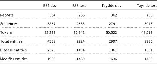
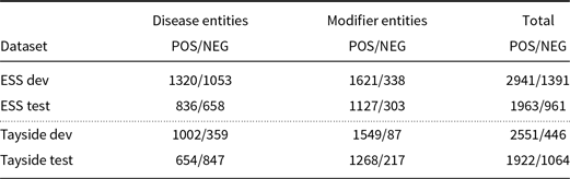
The Tayside data were received in parts, with development data being taken from the first part received and selected to match keywords for our target entities such as bleed and haemorrhage, as these are low frequency in routine reports. The Tayside test set was taken from the fourth part and was selected at random to produce a dataset with a distribution of entities that is more representative of the data we would expect to see in future. Though the parts were expected to be consistent in entity distribution, they varied, and this in addition to the selection criteria led to differences in disease entity distributions between the development and test data, as seen in Table 2.
The differences in the data due to the different sources (hospital-based register in the case of ESS vs. routine scans in the case of Tayside) is apparent in the number of tokens, sentences and entities in each dataset. ESS contains more annotated entities than Tayside, while Tayside contains a lot more tokens, but not sentences, than ESS. This suggests that the radiologists writing the Tayside reports used longer sentences. Because the Tayside data are not specific to stroke and tumour patients, it is not surprising that the number of entities annotated in them is lower.
As can be seen, entities include two types: disease observations and modifiers. The full set of disease observations are atrophy, haemorrhagic stroke, haemorrhagic transformation, ischaemic stroke, meningioma (mening tumour), metastatic tumour (metast tumour), microhaemorrhage, small vessel disease, stroke, subarachnoid haemorrhage, subdural haematoma and tumour. Modifiers designate a time or anatomical location for the disease and are further split into these two subtypes. Location can be cortical or deep, and time can be recent or old. Word tokens in a report can be associated with either a disease observation, a modifier or both, and all modifiers are associated with a disease via a relation. All entities appear with either a negated or non-negated annotation in the data. We note that we only annotate negation on entity and modifier annotations and therefore a token that is not an entity or modifier cannot be marked as negated.
There are many cases where the language expresses uncertainty rather than a clear positive/negative decision. For example, ‘it is not possible to exclude a small acute focal infarct’, while containing an overt negation cue word, is non-committal as to the presence of an infarct. Furthermore, sentences with no overt negation cue may also be non-committal, for example, ‘a small acute or subacute infarct may be missed”. In these cases, the annotators were instructed to mark the entities as negated, since the clinician has not clearly affirmed their presence, treating negation as assertion of whether the entity is definitely present or not. This treatment of negation is chosen due to our overall project objectives.
The annotation scheme was developed iteratively over the first tranch of the ESS development data with the annotators correcting the output of an early version of the EdIE-R rule-based system. This tranch of data (123 reports) was doubly annotated, inter-annotator agreement (IAA) was monitored and the annotators discussed and reconciled differences to create a jointly agreed initial dataset. This dataset was used to refine the rules in EdIE-R, which in turn fed into subsequent rounds of annotation. The remainder of the ESS development set was singly annotated, but the entire ESS test set (266 reports) was doubly annotated and IAA measured using precision, recall and F1 score. All of the Tayside data were subsequently singly annotated apart from the last 100 reports in the test set, which were doubly annotated to monitor IAA.
Since we only annotated negation for annotated entities, we cannot report IAA for negation and entities independently. We therefore report IAA for entities and negation combined. Since we are effectively computing IAA for NER with twice as many entity types, we report F1 score (Hripcsak and Rothschild Reference Hripcsak and Rothschild2005). The combined NER and negation IAA F1 scores on the ESS test set were
 $96.52$
and
 $95.52$
for Tayside. In order to get an additional estimate of IAA for negation detection, we can isolate negation scores for all entities the annotators agreed on. In this case, we report Cohen’s kappa (Cohen Reference Cohen1960) since we are effectively reporting agreement on binary classification, albeit on a subset of all entities. The negation IAA was
 $\kappa = 99.18$
for ESS and
 ${\kappa = 100.00}$
for Tayside, which equate to almost perfect and perfect agreement, respectively.
Dataset statistics

Table 1 lists the numbers of reports, sentences and words for each dataset, as well as total number of entities, disease entities and modifiers. The annotated reports in the ESS dataset were split into a development set (364 reports and 4332 entities) and an unseen test set (266 reports and 2924 entities). The Tayside data were split in a similar way (362 reports for development and 700 reports for evaluation). Rules were designed using the development portion of the ESS dataset.
For our neural network approaches, we use 80% of the ESS development documents for training our models and the remaining 20% of the ESS development documents as a validation set to choose the best hyperparameters for our models. Transfer learning where model weights trained on one dataset are used for another is an increasing focus in NLP (Mou et al. Reference Mou, Meng, Yan, Li, Xu, Zhang and Jin2016), as well as machine learning as a whole, and we also ran transfer learning-based experiments incorporating portions of the Tayside development documents into our training set for the neural networks, to evaluate adaptation to a novel dataset from that used for hyperparameter selection and training. We chose to train primarily on the ESS development data to allow comparison with the rule-based model. We then reported the performance of each of our models on both unseen test sets. The subsets of each dataset (ESS and Tayside) are as follows:
Development data, the part of the datasets that is used for development of the rule-based system, and for the training process (training and hyperparameter selection) of the machine learning models. The development data encompass both the training and validation data used by the machine learning algorithms;
Training data, the part of the datasets used to train the machine learning models;
Validation data, the part of the datasets used for hyperparameter selection for the machine learning approaches;
Test data, the part of the datasets that remains completely unseen by the models until test time.
Disease and modifier entity negation statistics across our datasets. The leading count is the number of non-negated occurrences (POS) followed by the number of negated occurrences (NEG)

4.1 Negation analysis
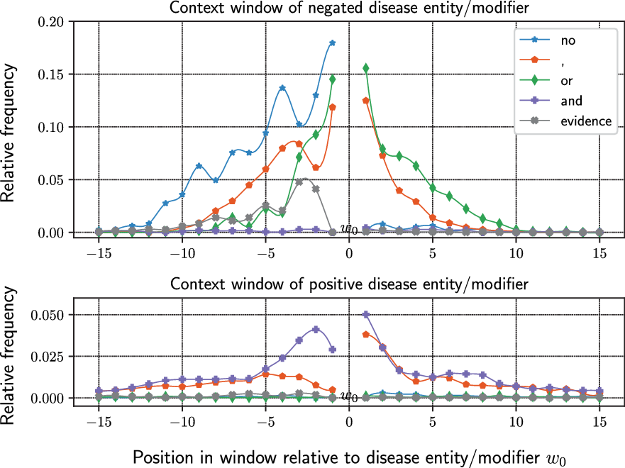
In this section, we begin by investigating how negation is expressed in brain imaging reports, in particular in the ESS development set. As we shall demonstrate, the manifestations of negation in such reports are clearly marked, making negation detection in this setting much more straightforward than negation detection in general purpose language, where it can be quite challenging. Namely, in the ESS dataset, negation is predominantly introduced explicitly using no and the negation scope is extended through connectives such as or, and and punctuation, as in the example ‘No acute haemorrhage, masses or extra-axial collections’. For brevity, we shall refer to all such tokens that are correlated with the introduction of negation as cues.
In Table 2, we tabulate the number of negated and non-negated disease entities and modifiers. For this study, negation cues were not explicitly annotated, so in the following analysis, we use the number of times a token appears in the context window of a negated disease or modifier annotation as a proxy for identifying negation cues.
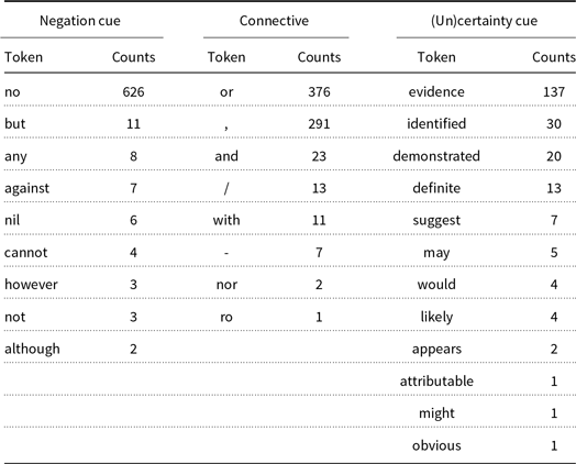
In order to get a better understanding of the types of negation cues used, in Table 3, we report the counts of cues that occur in the context of negated disease and modifier annotations. We group negation cues into three groups depending on their function. The first group of cues introduces negation (negation cue), the second extends negation to more entities through connectives (connective), and the third contains cues that express certainty or uncertainty ((un)certainty cue). Cues with such characteristics seem to be a common finding when working with radiology reports, see for example Peng et al. (Reference Peng, Yan, Sandfort, Summers and Lu2019, Table 2) which targets regular expression patterns such as no evidence of and or/and among others.
Counts of the most common tokens that surround a negated mention of a disease/modifier. Tokens are grouped into types depending on the manner with which we interpret them to interact with the mentions. They are ordered from top to bottom from most frequent to least frequent. The counts were constructed using a window of the 15 previous and 15 next tokens as context

The counts in Table 3 show that in the overwhelming majority of cases, negation is explicitly introduced using no with the remaining negation cues being rather scarce. From the middle column of our table, we extrapolate that negation scope is often extended to more entities through the use of connectives, such as or, and, nor, and the use of punctuation such as commas. In the last column, we tabulate more cues that potentially introduce certainty or uncertainty. For our study, we assume these cases also introduce negation, since annotators were instructed to mark all mentions of diseases and related modifiers that are not clearly indicated present as negated.
Lastly, we also inspected the coverage of these tokens, namely how many cases of negation in the dataset can be explained by finding a single occurrence of any of the cues listed in Table 3. We note that the presence of connectives does not necessarily imply negation; however, as we shall see in Figure 2, connectives such as or and comma occur much more frequently surrounding negated entities than positive entities. Hence, connectives contain a lot of information relating to negation in our dataset. We found that when inspecting a symmetric context window of 15 previous tokens and 15 next tokens surrounding a negated entity or modifier, we could not find any cues in the context in only 3 out of 1387 cases. When we narrowed down the context window to a symmetric window of five tokens, we found nine cases that could not be explained by the presence of a cue. This reinforces our belief that we are dealing with a rather degenerate case of negation compared to that of negation in a more general domain: we can get good results by relying on the presence of a rather small list of cues.
Negation cue distribution around negated (top graph) and positive (bottom graph) disease entities and modifiers for a selection of the most frequent cues from Table 3. We have plotted interpolating lines to highlight the relative increase and decrease in frequency depending on the position in the context window. We note that for the negated contexts seen in the top graph, no and evidence almost always precede the mention, while other cues appear both before and after it. Moreover, the appearance of no in the negated context can precede the entity by more than 10 tokens, while connectives such as and, or and comma appear in a closer context, suggesting that they are used to extend the scope of negation. As expected, the cues are more frequent in negated contexts than positive contexts as can be seen by comparing the graphs (note that the y-axis is on a different scale).

Our above interpretation of connectives extending negation scope becomes more evident when taking into account the top graph in Figure 2. The frequencies plotted are relative, in the sense that they are obtained by dividing the counts of our selected negation cues (no, comma, or, and, evidence) at a specific position in the context window by the number of non-disease entity/modifier tokens aggregated over the whole window. This calculation is performed twice, once for negated context windows (top graph) and once for positive context windows (bottom graph). Therefore, the graph captures both the distribution of cues around a disease entity or modifier
 $t_0$
in the context window, as well as their relative frequency of occurrence. As can be seen, no can precede the negated entity by more than 10 tokens, while connective cues such as or and comma appear closer to the negated disease and modifier annotations. Moreover, no is by far the most common negation cue with connectives being the next most common. Lastly, we turn to the bottom graph that shows the relative frequencies of negation cues in positive contexts. As expected, negation cues in non-negated contexts are rare, with the exception of and and comma which can be used in positive contexts as well.
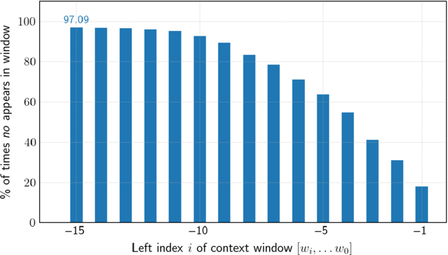
Given how commonly no occurs in the context of negated disease entities and modifiers, we now assess how often we can attribute negation to its appearance. As can be seen in Figure 3, no can be found in the 5 tokens preceding an entity around 50% of the time and in the preceding 15 tokens 97.09% of the time. This reinforces our understanding that negation is introduced explicitly and such negation cues are the most salient for negation detection.
Percentage of times negation of a disease entity or modifier
 $t_0$
can be explained by finding an occurrence of the negation cue no in the n preceding tokens. The graph can be interpreted as the cumulative value of the blue curve in the top graph of Figure 2, being aggregated from index 0 to
 $-15$
.

The simplicity and direct way with which entities are negated in the ESS dataset comes as no surprise when one considers the purpose of clinical text, namely, to communicate observations and diagnoses from a CT or MRI scan quickly and accurately to other clinicians. It is, however, not obvious that all teams of clinicians will communicate findings and express uncertainty in exactly the same way as that in the ESS dataset. For example, we saw earlier that not only occurs in the context of a negated word three times in the ESS dataset. Quite clearly, we could have a dataset where not is used to introduce negation commonly and in a variety of ways, a scenario which should give our current machine learning models difficulties, given they only have three examples to learn from. In the following section, we shall introduce our models and investigate the following question: how well do machine learning models trained only on the ESS dataset transfer to the unseen Tayside dataset?
5. Negation detection algorithms
In this section, we describe each of the approaches (three rule-based algorithms vs. two neural network algorithms) we used for negation detection in radiology reports in more detail.
5.1 Existing rule-based methods: pyConText and NegBio
NegEx is an NLP algorithm designed for negation detection (Chapman et al. Reference Chapman, Bridewell, Hanbury, Cooper and Buchanan2001). ConText (Harkema et al. Reference Harkema, Dowling, Thornblade and Chapman2009) is a generalisation of the NegEx algorithm, and here we adapted a Python implementation of ConText called pyConText for use with our dataset as a baseline. The algorithm uses a list of targets, for example, disease names, and a list of modifiers that are applied to these targets, for example, negation.
To use the pyConText algorithm with our dataset, we created a list of targets based on the diseases in our dataset. To create the same output format as that of the other models compared in this paper, we made a separate target list of our anatomical location and temporal information entities. We used the modifier list distributed with the algorithm; however, as we are only interested in negation of our entities, we removed all modifiers from this list that were not involved in assigning negation.
These target lists use regular expressions (Regex) for identification of targets. To create the Regex for each target, the phrases identified by the expert in our reports are used in an or arrangement. For example, for the target microhaemorrhage, an expert has identified it appearing in the reports through the use of the phrases micro bleeds and micro haemorrhage, leading to the Regex micro haemorrhage
 $|$
micro bleeds.
From the pyConText output, negation information is applied on the word level, and this is combined with the entity data without negation information from the manually annotated data for the final output.
For our second baseline we used NegBio, and to use the NegBio (Peng et al. Reference Peng, Wang, Lu, Bagheri, Summers and Lu2017) algorithm with our dataset we added targets from our dataset to the existing text target files, to ensure the NER part annotated all our entities. The annotations were then pruned so we were left with only the ones that matched with the manually annotated entities, and these were fed to the NegBio negation algorithm which adds negation information for each annotation.
For both of these methods, we did not change any rules or logic for the negation detection part of the algorithms, focusing only on ensuring they effectively worked with our datasets and target entities. This was to allow comparison of our custom-built rule-based model with out-of-the-box models.
5.2 Rule-based model (EdIE-R)
The EdIE-R rule-based system has a pipeline architecture where mark-up is added by each component feeding on information provided by earlier processing. Early linguistic processing components include sectioning, tokenisation, sentence-splitting, part-of-speech tagging and lemmatisation. During these early stages, negation cue words, such as no, not, never and nor, are marked as negated. At this point, the main information extraction components are applied, that is NER to mark up the entities, and relation extraction, which links disease entities and modifiers. In between these two steps, a shallow syntactic analysis known as chunking (Grover and Tobin Reference Grover and Tobin2006) is performed followed by rules to determine the scope of negation.
In a simple case such as ‘No obvious mass lesion’, the chunker establishes that this is a noun group, and negation, encoded as an attribute in the XML data structure, is propagated from No to the entire noun group. As mass lesion has already been identified by NER as a disease entity, this entity is marked as negated. Other cases require the chunker to recognise an embedded structure for noun groups, for example, where of-phrases act as noun modifiers (‘No evidence of metastatic disease’) or disjunctive structures (‘No acute haemorrhage, masses or extra-axial collections’) or a combination of the two (‘No evidence of acute infarct or bleed’). In these cases, the negation is propagated to the entire noun group, thereby defining the scope of the negation cue.
Elsewhere, the negation originates in a verb group and scopes over related noun groups, for example, ‘This does not show significant mass effect’ or ‘A small recent infarct cannot be detected’. In such cases, the identity of the verb is significant: in the above examples, negated show and detect lead to entities in their scope being identified as negated, but in ‘The cerebellar haematoma has not increased in size’, the haematoma entity should not be negated.
Our treatment of negation does not identify uncertainty, treating uncertain cases as negative, and the EdIE-R negation rules were formulated accordingly. In the remainder of this paper, we refer to this method as EdIE-R-Neg.
5.3 Neural network approaches
In this section, we will outline our two neural network approaches. We create word embeddings to encode each sentence’s lexical information. In order to encode entity information for the target entity, we suppress the lexical information contained in the word tokens that represent the entity and only include an entity surrogate embedding, ENT. Namely, we include a learned embedding that encodes whether the tokens are an entity. If an entity uses more than one token, for example, ‘ischaemic stroke’, both of these tokens are replaced with a single ENT token. We found using surrogates for entity phrases in this way improved our results on the validation set, likely as the ratio of negated to non-negated entities is highly variable when split by entity and does not generalise.
Additionally, we pad the input to a prespecified maximum input length using a reserved PAD token that has its own embedding. Lastly, we use the token UNK for any word not in our vocabulary. The vocabulary is built from the development data and we drop the least frequent 3% of the total words to train the UNK token embedding. We lowercase all words in our datasets.
These embeddings are fed through the networks as input. Both networks have an output layer with a sigmoid activation for binary classification. We use binary cross-entropy as our loss function. We train using the Adam (Kingma and Ba Reference Kingma and Ba2015) optimiser with exponential decay rates
 $\beta_1=0.9$
and
 $\beta_2=0.999$
. We randomly initialised word embeddings to be Gaussian
 $\sim \mathcal{N}(0, 1)$
. We train until there is no improvement in F1 score on the validation data, a held out split of the development data.
The model is trained and evaluated using data manually annotated by human experts. The development data were split into 80% training and 20% validation. Models were run five times with random initialisations, with an average F1 score being used for hyperparameter selection and reported in the summary tables. For Tables A.1 and A.2 which are split by entity type, we use the model that had the highest F1 score on the validation set using the chosen hyperparameters. We conduct a grid search over hyperparameters of embedding size, number of layers and hidden layer size for each neural network model, more details are given in the respective sections.
5.4 Feedforward Neural Network Model (FFNN-Neg)
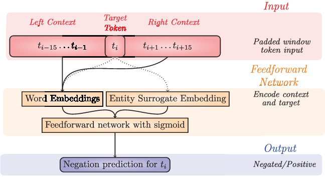
Motivated by our analysis of the distribution negation markers can have around negated entities as demonstrated in Figure 2, we use a large symmetric input window for our feedforward network. As can be seen in Figure 4, in order to predict if token
 $t_i$
is negated, we concatenate its context window of 15 tokens from the left and 15 tokens from the right and feed it to our network. If the input is shorter on either side, we pad it using a reserved PAD token that has its own embedding.
In order to encode entity information for the target token, we include a learned embedding that encodes the word token if the current input is not an entity, or the surrogate ENT token if it is an entity. After encoding the target token and its context, we concatenate the embeddings and feed them through a feedforward network with a hidden layer of dimensionality 128 and a ReLU non-linearity. We apply dropout of
 $0.5$
to the input and the hidden activation and normalise the hidden activation using Layer Normalisation (Ba, Kiros, and Hinton Reference Ba, Kiros and Hinton2016). The feedforward network has a single output with a sigmoid activation for binary classification.
FFNN-Neg architecture description. Given we wish to predict whether a target input
 $t_i$
is negated, we feed a padded context window surrounding the target token to the network. To encode entity information, we replace the tokens of an entity with a single surrogate ENT token. We feed the concatenation of the embeddings of the context window through a feedforward network with a single hidden layer and a sigmoid output layer for negation prediction.

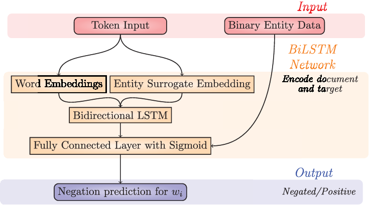
Token data are input for a word embedding and entity surrogate embedding, to which dropout of 0.5 is applied. These are used as input to a bidirectional LSTM. The hidden state of the LSTM is concatenated with Binary Entity Data for input into a fully connected layer with sigmoid activation for negation prediction.

In addition to hyperparameter details already specified in the introduction, we set our embedding size to 100 and used a single hidden layer with 128 hidden units, as we found these settings to give the best F1 score on the validation set. We use a batch size of 4096 context windows, which corresponds to a batch size of approximately 256 sentences assuming an average sentence length of 16 tokens. We train until no improvement on negation detection F1 score is obtained for 500 parameter updates on the held-out split of the development set. From here on, we refer to this model as FFNN-Neg.
5.5 LSTM-based model (BiLSTM-Neg)
As shown in Figure 5, the BiLSTM-Neg model consists of a bidirectional LSTM followed by a fully connected layer. Two inputs were created for the model, a word embedding and a binary measure of whether the token is an entity. The target output is an array of binary outputs, one for each token, of whether the token should be negated. Models were built in Python using the PyTorch (Paszke et al. Reference Paszke, Gross, Chintala, Chanan, Yang, DeVito, Lin, Desmaison, Antiga and Lerer2017) machine learning library. The Adam optimiser (Kingma and Ba Reference Kingma and Ba2015) was used with a learning rate of
 $\alpha=0.001$
and a weight decay of
 $0.0001$
. We apply a batch size of 32 documents.
The best model consisted of a two-layer LSTM of hidden size 128 using a 300-dimension word embedding to which a dropout of 0.5 has been applied. The final hidden state of the LSTM layer was concatenated with the binary entity measure to create the input for a fully connected layer, after which a sigmoid activation was applied to create the output to which threshold of 0.5 is applied to turn the float values into a binary measure. Negation predictions for entity tokens are combined with the entity types (without negation information) from the manually annotated reports for the final output. From here on, this model is referred to as BiLSTM-Neg.
6. Evaluation and results
All five models described above were run over the two test sets (ESS test and Tayside test) with the manually annotated word and entity data as input (without negation attributes for entities). The negated entity output for each algorithm and the manually annotated entities (with negation specified) were then converted to BIO ConLL format to evaluate using the CoNLL (Tjong Kim Sang Reference Tjong Kim Sang2002) perl evaluation script.Footnote b This is used for computing precision, recall and F1 score both as a total and per-entity type for diseases and modifiers separately. Negative entities were taken as the positive class. We report 95% confidence intervals for precision and recall of the rule-based models and the mean
 $\pm$
1 standard deviation over five runs with different random seeds for the machine learning models.
Overall negated entity (n. 961) results on the ESS test set. We report precision (positive predictive value), recall (sensitivity) and F1 score (harmonic mean of precision and recall) for negative annotations as well as 95% confidence intervals for precision and recall in parentheses for rule-based systems and the mean
 $\pm 1$
standard deviation of five runs with different random seeds for machine learning models. Bold text indicates the highest performing model overall.

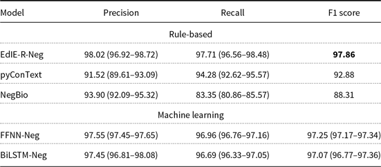
Table 4 shows the results for negated entities on the ESS test dataset for each of the models. The rule-based model, EdIE-R-Neg, and the two machine learning models, BiLSTM-Neg and FFNN-Neg, perform similarly, achieving F1 scores within a point. Each model performed better in precision than recall, likely due to a larger number of non-negated entities in the dataset. However, while the confidence intervals for precision and recall for the rule-based model overlap with one standard deviation from the mean of the machine learning models, meaning we lack confidence of the superiority of the EdIE-R-Neg model in these individual aspects, the F1 score for EdIE-R-Neg is higher than one standard deviation above the mean for both machine learning models, indicating EdIE-R-Neg will be the higher performing model for the majority, if not all, runs of the machine learning models.
Of the machine learning networks, FFNN-Neg looks to have the higher performance with higher mean scores for precision, recall and subsequently F1 score. However, this is inconclusive due to the mean scores of FFNN-Neg falling within one standard deviation of BiLSTM-Neg scores, meaning for any one run there is a large chance of either model having higher performance.
As expected, due to being developed on different datasets, the two existing rule-based methods, pyConText and NegBio, had weaker performance than those developed on the ESS development data, with NegBio particularly struggling with recall. pyConText shows a bias towards negated entities leading to a higher recall than precision, indicating that its negation rules are too broad for this dataset.
Overall negated entity (n. 988) results on the Tayside test set. We report precision (positive predictive value), recall (sensitivity) and F1 score (harmonic mean of precision and recall) for negative annotations as well as 95% confidence intervals for precision and recall in parentheses for rule-based systems and the mean
 $\pm 1$
standard deviation of five runs with different random seeds for machine learning models. Bold text indicates the highest performing model overall.

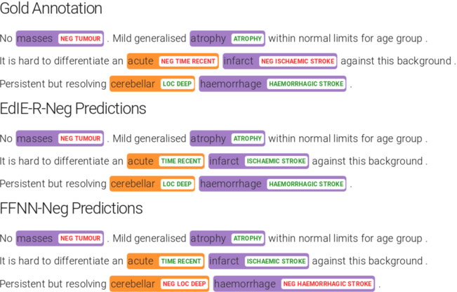
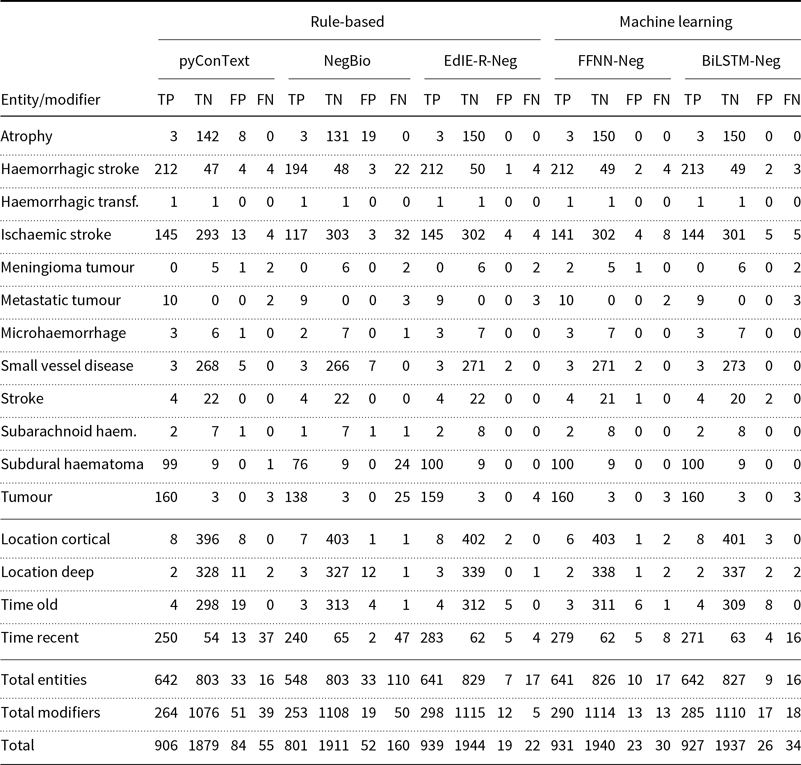
Largely, the misclassifications on the ESS test set made by the custom-built models, EdIE-R-Neg, FFNN-Neg and BiLSTM-Neg, were very similar, but there are some key differences. BiLSTM makes a number of errors for the modifier entity of time recent, missing more of the negated instances than FFNN-Neg, while EdIE-R-Neg makes less errors than both. Additionally, the machine learning models perform worse than EdIE-R-Neg on each of the other modifier entities. Examples of misclassifications made are shown in Figure 6.
Example negation detection output of EdIE-R-Neg and FFNN-Neg on synthetic data. Diseases are represented in purple and modifiers in orange. Negation is marked as NEG in the tag. Both systems get the first two sentences correct. Correctly tagging the third sentence relies on understanding that ‘hard to differentiate x’ implies that x is likely not present, something both EdIE-R-Neg and FFNN-Neg fail. FFNN-Neg gets the tags of the last sentence wrong presumably by relying on the presence of but or information that this is a haemorrhagic stroke entity, which is more commonly negated than not.

There were a few key entities where NegBio made most of its misclassifications, spread across disease and modifier entities. PyConText followed a more similar pattern of error to our models, but greater in number, particularly for modifier entities.
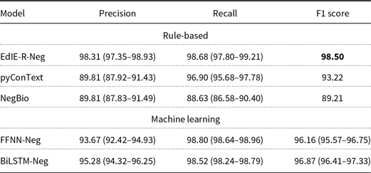
Table 5 shows the results for negated entities on the Tayside test set. Similar to the ESS test set, EdIE-R-Neg outperforms the other approaches in precision and F1 score; however, for recall the margin is small between all three approaches, with FFNN-Neg scoring marginally higher and the confidence interval for EdIE-R-Neg overlapping with one standard deviation from the mean of the machine learning models meaning we lack confidence of any model’s superiority on any one run of the machine learning models.
In contrast to the ESS test set, BiLSTM-Neg achieves a higher F1 score than FFNN-Neg due to a stronger precision; however, we draw no definite conclusion of superiority as one standard deviation below the mean for BiLSTM-Neg F1 score is lower than one standard deviation above the mean for FFNN-Neg F1 score, meaning there is a reasonable chance of either model having higher true performance. Additionally, FFNN-Neg scored higher than BiLSTM-Neg on recall, though the margin is small.
Both machine learning models perform better on recall than precision, indicating a bias towards over-prediction of negated entities, similar to the last sentence in the example in Figure 6. The decrease in precision led to a drop on F1 score and overall performance when compared to the performance on the ESS test set. The cross-training experiments below describe how this drop is reduced through addition of Tayside development data.
NegBio has a more balanced performance in contrast to the ESS test set, while pyConText continues to show a bias towards negated entities with a greater gap between a high recall and low precision compared to results on ESS test.
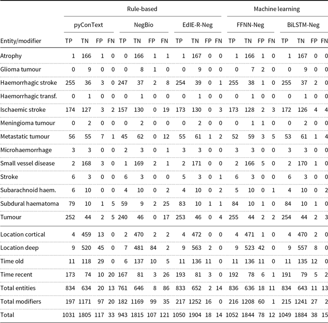
FFNN-Neg and BiLSTM-Neg followed a similar pattern of errors on the Tayside test set, with the exception of FFNN-Neg making a much greater number of errors on modifier entities, in particular location deep.
As on the ESS test set, pyConText makes misclassifications largely on the same entity types as the machine learning models, but with a greater number of errors on modifier entities. NegBio made higher numbers of misclassifications on a number of entities; however, a high proportion of its errors were made on the same entity, location deep, as FFNN-Neg made a high proportion of its errors on.
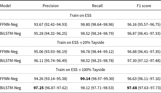
Effect of training on additional Tayside data on reported Tayside test scores (transfer learning). The scores reported are the mean over five runs with different random initialisation seeds and the range reported in parentheses is a standard deviation below and above the mean. Bold text indicates the highest performing model for each metric.

As expected due to training on data more similar to the test set, Table 6 shows that adding Tayside data to the ESS training data (transfer learning) increases the F1 scores of the machine learning models on the Tayside test set, particularly for Bi-LSTM-Neg which consistently improved on adding 20% and then 100% of Tayside development data.
The improvement for BiLSTM-Neg came from increases in precision (ESS only: 95.28; +20% Tayside: 96.11; +100% Tayside: 97.25) where previously both machine learning models were weak, giving a more equal balance between precision and recall. While recall did dip slightly from 98.52 to 98.12 for BiLSTM-Neg on adding 100%, this was a smaller drop and largely the high recall was maintained.
A drop in precision from 95.06 with 20% Tayside added to 94.26 with 100% Tayside added for FFNN-Neg led to a fall in F1 score from 96.88 to 96.63, despite recall increasing from 98.78 to 99.14. This is in contrast to the behaviour of BiLSTM-Neg (ESS only: 95.28; +20% Tayside: 96.11; +100% Tayside: 97.25) and the behaviour of FFNN-Neg on adding 20% Tayside (ESS only: 93.67; +20% Tayside: 95.06; +100% Tayside: 94.26), which improved upon a weakness in precision. Despite the increases in F1 score, both models remain weaker in performance than EdIE-R-Neg (EdIE-R-Neg: 98.50; BiLSTM-Neg: 97.68; FFNN-Neg: 96.88).
7. Discussion and further work
Through summing the true and false counts in Tables A.1 and A.2 in Section A in the Appendix, we see differences in total counts of entities between the ESS and Tayside datasets, such as for metastatic tumour (ESS test set: 12; Tayside test set: 119), as well as ratios of negated to non-negated entities (Ischaemic Stroke - ESS test set: 149:316; Tayside test set: 176:130). The difference is largely due to ESS being reports from scans conducted as part of a stroke study, while Tayside are routine scans. This may account for the imbalance that occurs between precision and recall on the Tayside test set for the machine learning models when training solely on ESS development data.
Negation patterns between the ESS and Tayside datasets are likely to be similar, for reasons including their source and the annotation process; therefore, it is unsurprising that methods developed on the ESS dataset, such as EdIE-R-Neg, score higher in F1 score on the Tayside test set than the existing rule-based systems developed on other datasets, pyConText and NegBio. PyConText and NegBio were also developed on clinical reports, and their lower performance compared to our models on the ESS and Tayside datasets indicates that even within the same domain generalisation is difficult.
We have shown that introducing a small amount of the novel dataset, Tayside, into training data can improve performance on an unseen subset of the Tayside dataset, increasing precision and reducing the deficit in overall performance to EdIE-R-Neg. As discussed negation patterns for the ESS and Tayside datasets are likely to be similar, and we hypothesise that on a novel dataset where the negation patterns differ more greatly to the development dataset that adaption of the neural network method will be quicker and more effective compared to a rule-based system. Future work will aim to test the hypothesis that a neural network pretrained on ESS development data and fine-tuned on the novel dataset would outperform EdIE-R-Neg. The i2b2 clinical dataset (Uzuner et al. Reference Uzuner, South, Shen and DuVall2011) is a strong candidate for the novel dataset.
In this work, we eliminated the time needed to tune hyperparameters for adaption to the Tayside dataset using the same model architecture selected from experiments on the ESS dataset only, and future work could further reduce the time taken to adapt to a new dataset through only fine-tuning the fully connected top layer of BiLSTM-Neg, or the final layer of FFNN-Neg, instead of the whole network.
Another common way to increase performance of natural language models is to use pretrained embeddings from much larger datasets. Pretrained word embeddings were tested in early versions of our neural network models without much success, and other work has also demonstrated inconclusive performance gains using either word or contextual embeddings that are not domain specific and instead trained on unrelated datasets (Cornegruta et al. Reference Cornegruta, Bakewell, Withey and Montana2016; Alsentzer et al. Reference Alsentzer, Murphy, Boag, Weng, Jindi, Naumann and McDermott2019). However, our datasets will grow as we receive more reports and pretraining embeddings on the larger dataset is worth revisiting, as well as fine-tuning contextual domain-specific embeddings from the recently available clinical BERT (Alsentzer et al. Reference Alsentzer, Murphy, Boag, Weng, Jindi, Naumann and McDermott2019).
Additionally, the gap in performance between EdIE-R-Neg and the machine learning models could be closed further through addition of a couple of key rules which could be explored in further work. Using rules, such as regular expressions like (no evidence of – no evidence of developing) entity, in post-processing has been found to increase performance over either method separately (Peng et al. Reference Peng, Yan, Sandfort, Summers and Lu2019). Similar rules tailored to the errors made could be used instead of the preprocessing outlined in the following paragraphs to address where the machine learning approaches struggle with modifier entities.
Ensemble-based algorithms use multiple systems to obtain better predictive performance than any single constituent system on it’s own (Polikar Reference Polikar2006) and are another way performance could be increased. However, due to similarities in performance by entity type and subtype, the specific errors made by the systems may overlap significantly, and so improvements might be marginal for the approaches and datasets in this paper.
To further reduce the numbers of misclassifications made by our models, it may be useful to target certain entities. Modifier entities like time recent and location deep had more errors than other entities, and further work could investigate preprocessing methods that may give more information on these entities to the machine learning models.
From the literature, we were expecting NegBio to outperform pyConText (Peng et al. Reference Peng, Wang, Lu, Bagheri, Summers and Lu2017). The weaker performance of NegBio came from a lower recall, indicating that non-negated entities were over-predicted, possibly due to negation cues in our dataset not present in that in which NegBio was developed. This is in contrast to pyConText which over-predicted negation. That a few key entities provided most of the errors for NegBio indicates there might be some key rules missing that are needed for the ESS and Tayside datasets more than other datasets.
8. Conclusion
We illustrate that negation detection, when conceptualised as a binary problem of presence versus non-presence, is a task that is relatively straightforward when working with radiology reports. We demonstrate this is the case, by showing that both rule-based, specifically ones optimised for a dataset, and neural network approaches can perform highly accurately. The lower complexity of the task is also shown by the high performance of a relatively simple feedforward network, along with using training examples numbering only in the thousands.
Both machine learning alternatives to the rule-based EdIE-R-Neg proved effective, achieving very similar F1 score performance on the ESS test set (EdIE-R-Neg: 97.86; BiLSTM-Neg: 97.07; FFNN-Neg: 97.25), with EdIE-R-Neg overall performing strongest. The pattern was similar for the Tayside test set (EdIE-R-Neg: 98.50; BiLSTM-Neg: 96.87; FFNN-Neg: 96.16); however, the gap between the machine learning models and EdIE-R-Neg was larger. On our datasets, all three models outperformed the two baseline existing rule-based models, pyConText and NegBio, demonstrating the effectiveness of custom-built models for specific datasets and indicating the difficulty in generalisation between medical datasets.
The performance deficit of the machine learning models on the Tayside test set to EdIE-R-Neg was reduced through addition of Tayside data to the training data of the neural network models (BiLSTM-Neg: 97.68; FFNN-Neg: 96.88). BiLSTM particularly benefited from the additional data, largely in precision.
Financial support
The research reported on in this paper was funded by the MRC Mental Health Data Pathfinder Award (MRC - MC_PC_17209). Moreover, Alex and Grover have been supported by the Alan Turing Institute via Turing Fellowships (EPSRC grant EP/N510129/1). Whiteley was supported by an MRC Clinician Scientist Award (G0902303) and is supported by a Scottish Senior Clinical Fellowship (CAF/17/01). Sudlow is Chief Scientist of UK Biobank and Director of Health Data Research UK Scotland. We would like to thank our funders for their support.
Additionally, we are grateful to The Health Informatics Centre (HIC), University of Dundee for providing anonymised brain imaging reports from NHS Tayside.
Availability of Data and Software
The annotated ESS corpus used for this research was created with funding from the Wellcome Trust. It is available for research uses on application to Prof. Cathie Sudlow (email: Cathie.Sudlow@ed.ac.uk) to bona fide researchers with a clear analysis plan, in line with the Wellcome Trust policy on data sharing.Footnote c We are in the process of creating a release of EdIE-R free for research purposes.Footnote d For more information, contact Dr. Beatrice Alex (email: balex@ed.ac.uk).
A. Result tables split by entity
Comparison of results for all models on the ESS test set broken down by disease and modifier entities including total counts. We take negation to be the positive class, therefore TP (True Positives) are correctly predicted negated disease and modifier entities while TN (True Negatives) are correctly predicted non-negated disease and modifier entities

Comparison of results for all models on the Tayside test set, as well as summary data for disease and modifier entities combined. We take negation to be the positive class, therefore TP (True Positives) are correctly predicted negated disease and modifier entities while TN (True Negatives) are correctly predicted non-negated disease and modifier entities