2. Problem formulation

We consider first the fixed-flux variant of the general problem described by Michelin & Lauga (Reference Michelin and Lauga2014). A sphere of radius $a$ is suspended in a solution of an otherwise uniform concentration, say $\mathscr{C}_{\infty }$ . Due to surface reaction, the particle emits solute at a prescribed rate $\mathscr{A}$ , which in general varies along the particle boundary; it is assumed to be axially symmetric. The interaction energy between the solute and the boundary, characterized by the length scale ${\it\lambda}$ , is comparable with the thermal energy $kT$ . Our goal is the calculation of the steady-state velocity acquired by the particle due to a non-uniform boundary distribution of $\mathscr{A}$ . The characteristic value of the excess-solute concentration, relative to the ambient value, is $\mathscr{C}=\Vert \mathscr{A}\Vert a/D$ , where $\Vert \mathscr{A}\Vert$ is some representative value of $\mathscr{A}$ and $D$ is the solute diffusivity. The interaction of the solute with the particle boundary is represented as a body force on the fluid, whose magnitude is of order $kT\mathscr{C}/a$ ; balancing this force with the viscous stress in the $O({\it\lambda})$ -wide interaction layer provides the pertinent velocity scale, namely

(2.1) $$\begin{eqnarray}\frac{\Vert \mathscr{A}\Vert kT{\it\lambda}^{2}}{{\it\eta}D},\end{eqnarray}$$

where ${\it\eta}$ is the solution viscosity.

We employ the macroscale formulation of Michelin & Lauga (Reference Michelin and Lauga2014), appropriate to the limit where the interaction thickness ${\it\lambda}$ is small compared with $a$ . In that formulation the pertinent fields are the flow and the excess-solute concentration outside the interaction layer. 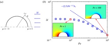In the dimensionless notation of Michelin & Lauga (Reference Michelin and Lauga2014) distances are normalized by $a$ , the excess-solute concentration by $\mathscr{C}$ , and the velocity scale $\mathscr{U}$ is chosen comparable with (2.1) (see below). The governing equations are written in a reference frame moving with the particle, where the problem is steady, using spherical coordinates in which the radial distance $r$ is measured from the sphere centre and the zenith angle ${\it\theta}$ is measured from the symmetry axis; see figure 1(a). For convenience, we actually use the alternative coordinate ${\it\mu}=\cos {\it\theta}$ .

Figure 1.

(a) Schematic. (b) Particle velocity ${\mathcal{U}}$ for the fixed-flux model, with $k({\it\mu})={\it\mu}$ and $M=1$ . Dashed line: large- $\mathit{Pe}$ approximation (3.22); symbols: computational results. The insets depict the solute-concentration distribution (scaled by the maximum surface concentration) as provided by the numerical solutions for $\mathit{Pe}=1$ and $\mathit{Pe}=100$ .

The excess concentration $c$ is governed by the advection–diffusion equation,

(2.2) $$\begin{eqnarray}\mathit{Pe}\,\boldsymbol{u}\boldsymbol{\cdot }\boldsymbol{{\rm\nabla}}c={\rm\nabla}^{2}c,\end{eqnarray}$$

where

(2.3) $$\begin{eqnarray}\mathit{Pe}=\frac{a\mathscr{U}}{D}\end{eqnarray}$$

is the Péclet number and $\boldsymbol{u}$ is the velocity field in the fluid, the imposed-flux condition,

(2.4) $$\begin{eqnarray}\frac{\partial c}{\partial r}=k({\it\mu})\quad \text{at }r=1,\end{eqnarray}$$

where $k=-\mathscr{A}/\Vert \mathscr{A}\Vert$ is an $O(1)$ scaled activity, and the attenuation condition,

(2.5) $$\begin{eqnarray}c\rightarrow 0\quad \text{as }r\rightarrow \infty .\end{eqnarray}$$

The velocity field $\boldsymbol{u}$ is governed by the Stokes equations, the far-field approach to a uniform velocity of magnitude ${\mathcal{U}}$ (see figure 1 a),

(2.6) $$\begin{eqnarray}\boldsymbol{u}\rightarrow -\hat{\boldsymbol{\imath }}\,{\mathcal{U}}\quad \text{as }r\rightarrow \infty ,\end{eqnarray}$$

wherein $\hat{\boldsymbol{\imath }}$ is a unit vector in the ${\it\theta}=0$ direction and ${\mathcal{U}}$ is the velocity of the particle relative to the fluid, and the condition that the particle is force free. The flow is animated by the slip condition,

(2.7) $$\begin{eqnarray}\boldsymbol{u}=M\boldsymbol{{\rm\nabla}}_{s}c\quad \text{at }r=1,\end{eqnarray}$$

wherein $M$ is the diffusio-osmotic slip coefficient and $\boldsymbol{{\rm\nabla}}_{s}$ is the surface-gradient operator. For an isotropic interaction potential $M$ is uniform, but may be either positive or negative; the scale $\mathscr{U}$ was chosen by Michelin & Lauga (Reference Michelin and Lauga2014) to make $M$ of unity magnitude, hence

(2.8) $$\begin{eqnarray}M=\pm 1.\end{eqnarray}$$

The goal is the calculation of the swimming velocity ${\mathcal{U}}$ as a function of $\mathit{Pe}$ and the distribution $k({\it\mu})$ . Because of the standard structure of a slip-driven Stokes-flow problem, ${\mathcal{U}}$ is obtained using the reciprocal theorem (Brenner Reference Brenner1964; Stone & Samuel Reference Stone and Samuel1996),

(2.9) $$\begin{eqnarray}{\mathcal{U}}=-\frac{1}{4{\rm\pi}}\hat{\boldsymbol{\imath }}\boldsymbol{\cdot }\oint _{r=1}\boldsymbol{u}\,\text{d}A,\end{eqnarray}$$

where $\text{d}A$ is a dimensionless areal element (normalized by $a^{2}$ ). Use of the axisymmetric slip (2.7) followed by integration by parts thus provides the formula

(2.10) $$\begin{eqnarray}{\mathcal{U}}=-M\int _{-1}^{1}{\it\mu}\,c(r=1,{\it\mu})\,\text{d}{\it\mu}.\end{eqnarray}$$

While the particle speed depends only upon the surface concentration of $c$ , one cannot avoid in general the solution of the flow problem: the concentration field is affected by the flow through the advection term in (2.2). Since this coupling between the flow and the solute concentration is nonlinear, so is the dependence of ${\mathcal{U}}$ upon both $\mathit{Pe}$ and $k({\it\mu})$ .

It should be noted that, in contrast to classical forced-convection problems (Acrivos & Goddard Reference Acrivos and Goddard1965), the Péclet number here does not involve an externally imposed velocity scale. Rather, it represents the intensity of interfacial chemical activity. Specifically, substitution of (2.1) into (2.3) implies that $\mathit{Pe}$ is of order

(2.11) $$\begin{eqnarray}\frac{\Vert \mathscr{A}\Vert kT{\it\lambda}^{2}a}{{\it\eta}D^{2}}.\end{eqnarray}$$

Michelin & Lauga (Reference Michelin and Lauga2014) used computations to analyse self-propulsion at arbitrary Péclet numbers and regular perturbations to obtain an analytic approximation for small Péclet numbers. In what follows, we employ singular perturbations to address the opposite asymptotic limit, $\mathit{Pe}\gg 1$ .

3. Large-Péclet-number limit

The advection–diffusion equation (2.2) suggests that in the large-Péclet-number limit the solute concentration is dominated by advection, so at leading order

(3.1) $$\begin{eqnarray}\boldsymbol{u}\boldsymbol{\cdot }\boldsymbol{{\rm\nabla}}c=0.\end{eqnarray}$$

Since the flow is steady, this implies that $c$ is a constant along the streamlines of the leading-order flow. Anticipating open streamlines, which originate and end at infinity, condition (2.5) then implies

(3.2) $$\begin{eqnarray}c\equiv 0.\end{eqnarray}$$

The nil result (3.2) is clearly incompatible with (2.4). This non-uniformity is associated with the singular nature of the large-Péclet-number limit, where the highest derivative is effectively multiplied by a small parameter. It suggests that a diffusive boundary layer is formed about the boundary $r=1$ ; in that thin layer, advection and diffusion of solute are comparable. It should be noted that the Stokes flow is coupled to the solute concentration $c$ only through its value at $r=1$ , and is accordingly ‘unaware’ of the steep gradient of $c$ near that surface; consequently, no boundary layer exists in the flow field.

3.1. Boundary-layer formulation

We denote the thickness of the layer by ${\it\delta}\;(\ll 1)$ . Its scaling with $\mathit{Pe}$ is readily obtained using dominant balances (Jülicher & Prost Reference Jülicher and Prost2009b ; Michelin & Lauga Reference Michelin and Lauga2014): from condition (2.4) we see that $c=O({\it\delta})$ in the layer. The slip condition (2.7) then implies the same scaling for the tangential velocity component $v$ , while the continuity equation in conjunction with the impermeability condition implies that the radial velocity component $u$ is of order ${\it\delta}^{2}$ . The advection–diffusion equation (2.2) thus yields ${\it\delta}=\mathit{Pe}^{-1/3}$ . It follows that in the boundary layer $c$ is $O(\mathit{Pe}^{-1/3})$ ; the velocity field $\boldsymbol{u}$ is of the same magnitude in the entire fluid domain, and then, given (2.9), so also is ${\mathcal{U}}$ .

The above scaling suggests the expansions $u=\mathit{Pe}^{-1/3}U+\cdots \,$ and $v=\mathit{Pe}^{-1/3}V+\cdots \,$ for the velocity components, where the rescaled components are $O(1)$ functions of $r$ and ${\it\mu}$ . Within the boundary layer we use the expansion

(3.3) $$\begin{eqnarray}c=\mathit{Pe}^{-1/3}C+\cdots \,,\end{eqnarray}$$

where the rescaled concentration $C$ is an $O(1)$ function of the stretched radial coordinate

(3.4) $$\begin{eqnarray}Y=\mathit{Pe}^{1/3}(r-1)\end{eqnarray}$$

and ${\it\mu}$ . In terms of the rescaled components, condition (2.7) becomes

(3.5a,b ) $$\begin{eqnarray}U=0,\quad V=-M(1-{\it\mu}^{2})^{1/2}f({\it\mu})\quad \text{at }r=1,\end{eqnarray}$$

where

(3.6) $$\begin{eqnarray}f({\it\mu})\stackrel{def}{=}\left.\frac{\partial C}{\partial {\it\mu}}\right|_{Y=0}.\end{eqnarray}$$

Since $U$ and $V$ vary on an $O(1)$ scale they are approximated in the boundary layer using Taylor expansions about $r=1$ , which, in view of (3.5a ), read

(3.7a,b ) $$\begin{eqnarray}U=(r-1)\left.\frac{\partial U}{\partial r}\right|_{r=1}+\cdots \,,\quad V=\left.V\right|_{r=1}+\cdots \,.\end{eqnarray}$$

Use of the leading-order continuity equation,

(3.8) $$\begin{eqnarray}\frac{\partial U}{\partial r}=\frac{\partial }{\partial {\it\mu}}[(1-{\it\mu}^{2})^{1/2}V],\end{eqnarray}$$

allows both approximations to be expressed in terms of $\left.V\right|_{r=1}$ . Substitution into the advection–diffusion equation (2.2) and making use of (3.5b ) thus yields the parabolic equation,

(3.9) $$\begin{eqnarray}M\frac{\partial ^{2}C}{\partial Y^{2}}=(1-{\it\mu}^{2})f({\it\mu})\frac{\partial C}{\partial {\it\mu}}-Y\frac{\partial }{\partial {\it\mu}}[(1-{\it\mu}^{2})f({\it\mu})]\frac{\partial C}{\partial Y},\end{eqnarray}$$

governing the boundary-layer solute concentration. It is supplemented by the boundary condition (cf. (2.4))

(3.10) $$\begin{eqnarray}\frac{\partial C}{\partial Y}=k({\it\mu})\quad \text{at }Y=0\end{eqnarray}$$

and the matching condition (see (3.2))

(3.11) $$\begin{eqnarray}C\rightarrow 0\quad \text{as }Y\rightarrow \infty .\end{eqnarray}$$

The boundary-value problem (3.9)–(3.11) is uncoupled from that governing the flow, and may be solved independently. In view of (2.10) there is actually no need to solve for the flow: once $C$ is known, the particle velocity is obtained from (2.10) and (3.3). It should be noted, however, that as $f({\it\mu})$ is related to $C$ through (3.6), (3.9) is a nonlinear equation.

The preceding boundary-layer problem appears to be similar to that governing the nutrient concentration about a squirming sphere (Magar, Goto & Pedley Reference Magar, Goto and Pedley2003; Michelin & Lauga Reference Michelin and Lauga2011). In the feeding problem, however, the slip distribution is prescribed, and is accordingly independent of the Péclet number; this results in a linear problem with a boundary-layer thickness that scales as the $-1/2$ power of that number.

3.2. Boundary-layer analysis

Following the analysis of a similar boundary-layer problem (Schnitzer, Frankel & Yariv Reference Schnitzer, Frankel and Yariv2014), our approach in confronting (3.9)–(3.11) is to calculate $C$ as if $f({\it\mu})$ were a prescribed quantity. The solution of the linear system (3.9)–(3.11) in conjunction with (3.6) then provides a nonlinear equation governing $C$ at $Y=0$ . Given (2.10) and (3.3), this interfacial distribution is all that we need to obtain the swimming velocity.

Our scheme is appropriate for the class of problems where the boundary layer does not detach; given (2.7) this necessitates that on the boundary $C$ is a strictly increasing or decreasing function of ${\it\mu}$ . With no loss of generality we assume the latter,

(3.12) $$\begin{eqnarray}f({\it\mu})<0.\end{eqnarray}$$

Given (3.10) and the vanishing of $C$ at the outer edge of the boundary layer, it appears plausible that for (3.12) to be satisfied $k({\it\mu})$ must be strictly increasing.

The parabolic equation (3.9) does not appear to be amenable to integral transform. We accordingly shift to stream-function coordinates (Levich Reference Levich1962), replacing the independent variables $(Y,{\it\eta})$ by $({\it\Psi},{\it\eta})$ , with

(3.13) $$\begin{eqnarray}{\it\Psi}=-Y(1-{\it\mu}^{2})f({\it\mu})\end{eqnarray}$$

(which is proportional to the Stokes stream function near $r=1$ ). On substituting this change of variables into (3.9), we find that $C({\it\Psi},{\it\mu})$ satisfies the equation

(3.14) $$\begin{eqnarray}\frac{\partial C}{\partial {\it\mu}}=M(1-{\it\mu}^{2})f({\it\mu})\frac{\partial ^{2}C}{\partial {\it\Psi}^{2}},\end{eqnarray}$$

while condition (3.10) becomes

(3.15) $$\begin{eqnarray}\frac{\partial C}{\partial {\it\Psi}}=-\frac{k({\it\mu})}{(1-{\it\mu}^{2})f({\it\mu})}\quad \text{at }{\it\Psi}=0;\end{eqnarray}$$

given (3.12), the decay condition (3.11) now applies as ${\it\Psi}\rightarrow \infty$ ,

(3.16) $$\begin{eqnarray}C\rightarrow 0\quad \text{as }{\it\Psi}\rightarrow \infty .\end{eqnarray}$$

The boundary-value problem (3.14)–(3.16) is naturally solved using a Fourier cosine transform, defined as

(3.17) $$\begin{eqnarray}{\hat{C}}({\it\omega},{\it\mu})=\left(\frac{2}{{\rm\pi}}\right)^{1/2}\int _{0}^{\infty }C({\it\Psi},{\it\mu})\cos ({\it\omega}{\it\Psi})\,\text{d}{\it\omega}.\end{eqnarray}$$

Application of this transform to (3.14)–(3.16) results in the first-order equation

(3.18) $$\begin{eqnarray}\frac{\partial {\hat{C}}}{\partial {\it\mu}}+M{\it\omega}^{2}(1-{\it\mu}^{2})f({\it\mu}){\hat{C}}=M\left(\frac{2}{{\rm\pi}}\right)^{1/2}k({\it\mu}).\end{eqnarray}$$

The complementary solution of (3.18) is $A({\it\omega})\text{e}^{-M{\it\omega}^{2}{\it\chi}({\it\mu})}$ , where

(3.19) $$\begin{eqnarray}{\it\chi}({\it\mu})=\int _{0}^{{\it\mu}}f(q)(1-q^{2})\,\text{d}q;\end{eqnarray}$$

given (3.12), ${\it\chi}({\it\mu})$ is strictly decreasing. A particular integral of (3.18) is

(3.20) $$\begin{eqnarray}M\left(\frac{2}{{\rm\pi}}\right)^{1/2}\int _{{\it\mu}_{0}}^{{\it\mu}}k({\it\xi})\text{e}^{-M{\it\omega}^{2}[{\it\chi}({\it\mu})-{\it\chi}({\it\xi})]}\,\text{d}{\it\xi}.\end{eqnarray}$$

The value of ${\it\mu}_{0}$ (and then $A$ ) is determined by the condition that ${\hat{C}}\rightarrow 0$ as ${\it\omega}\rightarrow \infty$ regardless of the value of ${\it\mu}$ . We now show that, upon choosing ${\it\mu}_{0}=M$ , this condition yields $A=0$ . Indeed, since the function ${\it\chi}$ is strictly decreasing this choice results in a negative power in the exponent appearing in (3.20), whereby the particular solution vanishes as ${\it\omega}\rightarrow \infty$ . Given (3.12), the sign of ${\it\chi}({\it\mu})$ is opposite to that of ${\it\mu}$ , implying that the exponent in the complementary solution diverges as ${\it\omega}\rightarrow \infty$ for a finite interval of ${\it\mu}$ values ( $0<{\it\mu}<1$ for $M=1$ ; $-1<{\it\mu}<0$ for $M=-1$ ). Since ${\hat{C}}$ must vanish in that limit for all ${\it\mu}$ , it follows that $A=0$ .

We conclude that ${\hat{C}}$ is provided by (3.20) with ${\it\mu}_{0}=M$ . By applying the inverse transform, interchanging the order of integrations and evaluation at ${\it\Psi}=0$ we obtain, upon substitution of (3.6) and (3.19), the following equation governing $C$ on the particle boundary (denoted $C({\it\mu})$ for brevity):

(3.21) $$\begin{eqnarray}C({\it\mu})=\frac{M}{\sqrt{{\rm\pi}}}\int _{M}^{{\it\mu}}\frac{k({\it\xi})\,\text{d}{\it\xi}}{\sqrt{\displaystyle M\int _{{\it\xi}}^{{\it\mu}}(1-q^{2})\frac{\text{d}C}{\text{d}q}\,\text{d}q}}.\end{eqnarray}$$

Since $C({\it\mu})$ is strictly decreasing, the local slip is directed in the $\pm {\it\theta}$ direction for $M=\pm 1$ . Given (2.10), this implies that the particle moves in the $\pm \hat{\boldsymbol{\imath }}$ direction. In the particle-fixed reference frame, the direction of the incident flow is then $\mp \hat{\boldsymbol{\imath }}$ . In view of the parabolic nature of the boundary-layer problem, the value of $C$ at a certain value of ${\it\mu}$ is only affected by the distribution of $C$ upstream. For $M=1$ this upstream distribution corresponds to the interval $({\it\mu},1)$ , while for $M=-1$ it corresponds to $(-1,{\it\mu})$ . Equation (3.21) is indeed consistent with this information-propagation property.

Equation (3.21) constitutes an integral equation governing $C({\it\mu})$ (cf. Acrivos & Chambré Reference Acrivos and Chambré1957). Upon expanding $C({\it\mu})$ in Legendre polynomials, $C({\it\mu})=\sum _{n=0}^{\infty }A_{n}P_{n}({\it\mu})$ , it is transformed into a nonlinear algebraic system governing the coefficients $\{A_{n}\}$ . This system may be solved using an iterative scheme when $C({\it\mu})$ is strictly decreasing. Once solved, the particle velocity is obtained using (2.10) and (3.3), yielding

(3.22) $$\begin{eqnarray}{\mathcal{U}}\approx -{\textstyle \frac{2}{3}}MA_{1}\mathit{Pe}^{-1/3}.\end{eqnarray}$$

For a given distribution $k({\it\mu})$ one needs in general to solve (3.21) separately for $M=\pm 1$ , resulting in two different distributions – say $C_{\pm }({\it\mu})$ . In the case where $k({\it\mu})$ is an odd function, however, it is readily verified from (3.21) that $C_{-}({\it\mu})=-C_{+}(-{\it\mu})$ . Given (2.10), the resulting particle velocities are opposite in sign. This, of course, is obvious by symmetry.

The asymptotic prediction (3.22) can be compared with a direct computational solution of (2.2)–(2.7), obtained using a spectral decomposition in the azimuthal direction and a stretched radial grid (see Michelin & Lauga (Reference Michelin and Lauga2014) for more details). As an example we consider the simple distribution $k({\it\mu})={\it\mu}$ . Since this function is odd, it is sufficient to solve (3.21) for $M=1$ ; we then obtain from (2.10) that $A_{1}=-0.86$ , whereby (3.22) gives ${\mathcal{U}}\approx 0.57\mathit{Pe}^{-1/3}$ . This result is in excellent agreement with the full numerical solution; see figure 1(b). The solute-concentration maps, shown in the insets, illustrate the transition from an essentially fore–aft symmetric distribution at weak convection to a boundary-layer structure at strong convection.

It should be noted that the use of the macroscale model of Michelin & Lauga (Reference Michelin and Lauga2014) within a boundary layer of dimensional thickness $a{\it\delta}$ implies that the underlying limit of that model, ${\it\lambda}\ll a$ , should be refined to ${\it\lambda}\ll a{\it\delta}$ . Moreover, the very derivation of the effective conditions (2.4) and (2.7) actually requires $({\it\lambda}/a)\mathit{Pe}\ll 1$ and $({\it\lambda}/a)^{2}\mathit{Pe}\ll 1$ respectively (Michelin & Lauga Reference Michelin and Lauga2014). As the boundary-layer thickness ${\it\delta}$ is $\mathit{Pe}^{-1/3}$ , it follows that the stringent condition that must be satisfied is ${\it\lambda}/a\ll \mathit{Pe}^{-1}$ . Michelin & Lauga (Reference Michelin and Lauga2014) estimated that ${\it\lambda}/a$ is between $10^{-5}$ and $10^{-3}$ , implying that the computations performed for the largest Péclet number employed herein ( $\mathit{Pe}=100$ ) still fall within the validity domain of the model.

4. Fixed-rate model

We now consider the fixed-rate model, where the rate constant $\mathscr{K}$ of a first-order kinetic relation is specified on the particle boundary (and is assumed to be axially symmetric). Since a characteristic rate of solute absorption is $\Vert \mathscr{K}\Vert \mathscr{C}_{\infty }$ , where $\Vert \mathscr{K}\Vert$ is a characteristic norm of $\mathscr{K}$ , the velocity scale (2.1) is replaced by

(4.1) $$\begin{eqnarray}\frac{\Vert \mathscr{K}\Vert \mathscr{C}_{\infty }kT{\it\lambda}^{2}}{{\it\eta}D}.\end{eqnarray}$$

The Péclet number is now of order (cf. (2.11))

(4.2) $$\begin{eqnarray}\frac{a\Vert \mathscr{K}\Vert \mathscr{C}_{\infty }kT{\it\lambda}^{2}}{{\it\eta}D^{2}}.\end{eqnarray}$$

The limit of short-range interaction is again governed by (2.2)–(2.7), except that (2.4) is replaced by

(4.3) $$\begin{eqnarray}\frac{\partial c}{\partial r}=k({\it\mu})(1+\mathit{Da}\,c)\quad \text{at }r=1,\end{eqnarray}$$

wherein

(4.4) $$\begin{eqnarray}\mathit{Da}=\frac{a\Vert \mathscr{K}\Vert }{D}\end{eqnarray}$$

is the Damköhler number and now $k=\mathscr{K}/\Vert \mathscr{K}\Vert$ , which is again an $O(1)$ distribution; since the first-order kinetics describe solute adsorbing onto the boundary, $k$ is here non-negative.

When addressing here the limit of large Péclet numbers care must be exercised. Given (4.2), one would typically envision large $\mathit{Pe}$ due to fast reaction (large $\Vert \mathscr{K}\Vert$ ) or large swimmers (large $a$ ). Since, however, both $\mathit{Pe}$ and $\mathit{Da}$ are linear in $a\Vert \mathscr{K}\Vert$ , the proper limit to consider is that where $\mathit{Da}$ becomes $O(\mathit{Pe})$ .

With a large Péclet number, one may naively expect the topology of the fixed-flux analysis, namely the trivial solution (3.2) with a non-zero excess concentration confined to a thin boundary layer. A dominant-balance inspection reveals, however, that no boundary-layer structure is compatible with condition (4.3). This apparent paradox is readily resolved by noting that, if

(4.5) $$\begin{eqnarray}\boldsymbol{u}=O(\mathit{Pe}^{-1})\quad \text{or asymptotically smaller},\end{eqnarray}$$

the advective term does not dominate (2.2). Approximation (3.1) is then rendered invalid, as is then (3.2); thus, no boundary layer is realized.

We therefore proceed under the a priori assumption (4.5). The scalings of $c$ and $\boldsymbol{u}$ are accordingly obtained by considering the dominant balances of (4.3) in the absence of a boundary layer. As it turns out, the only consistent balance is that between the last two terms in (4.3), implying that $c$ is $O(\mathit{Da}^{-1})$ . It should be noted, however, that this is not the velocity scaling, since the present balance implies a uniform leading-order value of $c$ (namely $-1/\mathit{Da}$ ) on the boundary, so the slip is triggered by the leading-order correction to the $O(\mathit{Da}^{-1})$ concentration. It follows from (4.3) that this correction is of order $\mathit{Da}^{-2}$ , thus providing the velocity scaling. With $\mathit{Da}=O(\mathit{Pe})$ , this is indeed compatible with (4.5).

As the fluid velocity is $O(\mathit{Pe}^{-2})$ it becomes evident that the leading-order transport is (counter-intuitively) unaffected by advection. Following the preceding arguments we postulate the expansions

(4.6a−c ) $$\begin{eqnarray}c=\mathit{Da}^{-1}c_{1}+\mathit{Da}^{-2}c_{2}+\cdots \,,\quad \boldsymbol{u}=\mathit{Da}^{-2}\boldsymbol{u}_{2}+\cdots \,,\quad {\mathcal{U}}=\mathit{Da}^{-2}{\mathcal{U}}_{2}+\cdots \,.\end{eqnarray}$$

At $O(1)$ , condition (4.3) yields

(4.7) $$\begin{eqnarray}c_{1}=-1\quad \text{at }r=1.\end{eqnarray}$$

From (2.2) we find that the leading-order concentration $c_{1}$ is harmonic. The solution that satisfies (4.7) and decays at infinity is the monopole

(4.8) $$\begin{eqnarray}c_{1}=-\frac{1}{r}.\end{eqnarray}$$

At $O(\mathit{Da}^{-1})$ , condition (4.3) reads

(4.9) $$\begin{eqnarray}\frac{\partial c_{1}}{\partial r}=k({\it\mu})c_{2}\quad \text{at }r=1.\end{eqnarray}$$

Substitution of (4.8) yields $c_{2}=1/k({\it\mu})$ at $r=1$ . It should be noted that there is no need to solve for $c_{2}$ in the fluid domain, where it is governed by an advection–diffusion equation. Indeed, using (2.10) we readily obtain

(4.10) $$\begin{eqnarray}{\mathcal{U}}_{2}=-M\int _{-1}^{1}\frac{{\it\mu}\,\text{d}{\it\mu}}{k({\it\mu})}.\end{eqnarray}$$

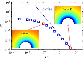
In figure 2 we compare the asymptotic approximation ${\mathcal{U}}\approx \mathit{Da}^{-2}{\mathcal{U}}_{2}$ with the computational solution. This is done for $M=1$ and the rate-constant distribution $k({\it\mu})=1+{\it\mu}/2$ , for which (4.10) yields ${\mathcal{U}}_{2}=2\ln 9-4\approx 0.3944$ . The computations were performed for $\mathit{Da}=\mathit{Pe}$ . At large $\mathit{Da}$ they indeed agree with the asymptotic approximation. The solute-concentration maps, shown in the insets, illustrate the transition at large $\mathit{Da}$ to the radially symmetric distribution (4.8).

Figure 2.

Particle velocity ${\mathcal{U}}$ for the fixed-rate model, with $k({\it\mu})=1+{\it\mu}/2$ and $M=1$ . Line: large- $\mathit{Pe}$ approximation; symbols: computational results, performed for $\mathit{Da}=\mathit{Pe}$ . The insets depict the solute-concentration distribution (scaled by the maximum surface concentration) as provided by the numerical solutions for $\mathit{Da}=1$ and $\mathit{Da}=50$ . Note the approach to a spherically symmetric distribution with increasing $\mathit{Pe}$ (cf. (4.8)).

5. Concluding remarks

We have analysed self-propulsion of a chemically reactive particle for large Péclet numbers. In the fixed-flux model, the excess-solute concentration is localized in a narrow boundary layer. Use of boundary-layer approximations reduces the coupled problem governing the nonlinear solute transport and fluid motion to the solution of an integral equation governing the interfacial solute concentration. In the fixed-rate model, we focused upon the limit of large swimmers or strong reaction, where the Damköhler number becomes comparable with the Péclet number. In that problem no boundary layer occurs, and solute advection actually diminishes with increasing $\mathit{Pe}$ .

The respective scaling of the dimensionless velocity with $\mathit{Pe}^{-1/3}$ and $\mathit{Da}^{-2}$ implies that the velocities (2.1) and (4.1), characteristic of the flow at moderate $\mathit{Pe}$ , are no longer representative at large $\mathit{Pe}$ . Rather, making use of (2.1) and (2.11) in the fixed-flux case and (4.1) and (4.4) in the fixed-rate case, we find instead the respective velocity scales (cf. Jülicher & Prost Reference Jülicher and Prost2009b )

(5.1a,b ) $$\begin{eqnarray}\frac{\Vert \mathscr{A}\Vert ^{2/3}(kT)^{2/3}{\it\lambda}^{4/3}}{{\it\eta}^{2/3}D^{1/3}a^{1/3}},\quad \frac{\mathscr{C}_{\infty }kT{\it\lambda}^{2}D}{{\it\eta}a^{2}\Vert \mathscr{K}\Vert },\end{eqnarray}$$

representing a transition from a size-independent velocity to ones that decrease with particle size. As the generic velocity scales (2.1) and (4.1) are non-representative at large $\mathit{Pe}$ , it follows that the dimensionless number $\mathit{Pe}$ itself, as provided by (2.11) and (4.2), does not constitute a genuine Péclet number, but simply a measure of the surface activity. This is reminiscent of electrokinetic phenomena at strong applied fields (Schnitzer & Yariv Reference Schnitzer and Yariv2012b ; Schnitzer, Frankel & Yariv Reference Schnitzer, Frankel and Yariv2013; Schnitzer et al. Reference Schnitzer, Frankel and Yariv2014) or due to imposed flows (Yariv, Schnitzer & Frankel Reference Yariv, Schnitzer and Frankel2011), where the generic Péclet number defined by Saville (Reference Saville1977) no longer represents the relative magnitudes of advection and diffusion.

The present work suggests two future directions. The first is a different analysis of the fixed-reaction-rate model, appropriate to the case where $\mathit{Pe}$ becomes large due to large solute molecules (small $D$ ). In that scenario, where $\mathit{Da}$ is $O(\mathit{Pe}^{1/2})$ , the boundary-layer thickness is $\mathit{Pe}^{-1/2}$ , with an identical scaling for the velocity field (so (4.5) is satisfied). The boundary-layer problem is then similar to that formulated in § 3.1, except that (3.10) is replaced by an inhomogeneous Robin condition.

The other direction involves the case where the chemical reactions produce ions, rather than neutral species. In that case the interaction layer is the Debye diffuse-charge layer. This problem is fundamentally different, as the interaction potential (namely the electric potential) is itself coupled to the ionic concentrations through Poisson’s equation. This ‘auto-electrophoresis’ problem therefore falls into the realm of electrokinetics (Moran, Wheat & Posner Reference Moran, Wheat and Posner2010). The macroscale description of that problem, appropriate to the limit of thin double layers, was developed by Yariv (Reference Yariv2011). It differs from the macroscale description of Michelin & Lauga (Reference Michelin and Lauga2014) in several fundamental aspects, the important one being the need to solve for the nonlinearly coupled transport of two fields (ionic concentration and electric potential). Solute advection then constitutes only one of several nonlinearities inherent in the problem. The macroscale model of Yariv (Reference Yariv2011) was solved in that paper using a linearization scheme, appropriate to the case of a nearly homogeneous particle. It is desirable to extend this solution with numerical computations, similar to those of Michelin & Lauga (Reference Michelin and Lauga2014), as well as a large-Péclet-number asymptotic analysis, comparable with that appearing in the present paper.