





1. Introduction
Evidence of scientists’ fascination for drop impacts can be traced back to the sketch of a water drop splashing onto a sheet of paper by Leonardo da Vinci in the margin of folio 33r in Codex Hammer/Leicester (1506–1510) (da Vinci Reference da Vinci1508). In particular, the striking patterns created by drop fragmentation, at high impact velocity, have attracted attention (Rein Reference Rein1993; Xu, Zhang & Nagel Reference Xu, Zhang and Nagel2005; Yarin Reference Yarin2006; Villermaux & Bossa Reference Villermaux and Bossa2011; Josserand & Thoroddsen Reference Josserand and Thoroddsen2016; Kim et al. Reference Kim, Wu, Esmaili, Dombroskie and Jung2020). Lower velocity impacts, although they do not cause drops to shatter, also give rise to a rich variety of phenomena (Worthington Reference Worthington1877a,Reference Worthingtonb; Chandra & Avedisian Reference Chandra and Avedisian1991; Yarin Reference Yarin2006; Thoroddsen, Etoh & Takehara Reference Thoroddsen, Etoh and Takehara2008; Josserand & Thoroddsen Reference Josserand and Thoroddsen2016). The rebound of drops on non-wetting substrates may be one of the most fascinating of such interactions (Richard & Quéré Reference Richard and Quéré2000; Richard, Clanet & Quéré Reference Richard, Clanet and Quéré2002; Tsai et al. Reference Tsai, Pacheco, Pirat, Lefferts and Lohse2009; Nair et al. Reference Nair, Staat, Tran, van Houselt, Prosperetti, Lohse and Sun2014).
Upon impact, the liquid first spreads (Philippi, Lagrée & Antkowiak Reference Philippi, Lagrée and Antkowiak2016; Gordillo, Sun & Cheng Reference Gordillo, Sun and Cheng2018) until it reaches its maximal extent (Clanet et al. Reference Clanet, Béguin, Richard and Quéré2004; Laan et al. Reference Laan, de Bruin, Bartolo, Josserand and Bonn2014; Wildeman et al. Reference Wildeman, Visser, Sun and Lohse2016; Gordillo, Riboux & Quintero Reference Gordillo, Riboux and Quintero2019). It then recoils, following a Taylor–Culick-type retraction parallel to the substrate (Taylor Reference Taylor1959; Culick Reference Culick1960; Bartolo, Josserand & Bonn Reference Bartolo, Josserand and Bonn2005; Deka & Pierson Reference Deka and Pierson2020; Pierson et al. Reference Pierson, Magnaudet, Soares and Popinet2020; Sanjay et al. Reference Sanjay, Sen, Kant and Lohse2022), and ultimately bounces off in an elongated shape perpendicular to the substrate (Richard & Quéré Reference Richard and Quéré2000; Yarin Reference Yarin2006; Josserand & Thoroddsen Reference Josserand and Thoroddsen2016).
Such rebounds abound in nature, as non-wetting surfaces provide plants and animals a natural way to keep dry (Neinhuis & Barthlott Reference Neinhuis and Barthlott1997; Quéré Reference Quéré2008), and are relevant in many industrial processes such as inkjet printing (Lohse Reference Lohse2022). In some applications, it is pertinent that drops ricochet off the surface, such as in self-cleaning (Blossey Reference Blossey2003), keeping clothes dry (Liu, Chen & Xin Reference Liu, Chen and Xin2008) and anti-fogging surfaces (Mouterde et al. Reference Mouterde, Lehoucq, Xavier, Checco, Black, Rahman, Midavaine, Clanet and Quéré2017a). However, in most cases, bouncing must be suppressed. For example, in cooling applications (Kim Reference Kim2007; Shiri & Bird Reference Shiri and Bird2017; Jowkar & Morad Reference Jowkar and Morad2019) and pesticide spraying in agriculture (Bergeron et al. Reference Bergeron, Bonn, Martin and Vovelle2000; He et al. Reference He, Ding, Li, Mu, Li and Liu2021; Gorin et al. Reference Gorin, Di Mauro, Bonn and Kellay2022). It is therefore natural to wonder when a drop stops bouncing.
Thus, when does the bouncing stop? On the one hand, Biance et al. (Reference Biance, Chevy, Clanet, Lagubeau and Quéré2006) found that heavy drops, i.e. drops larger than their gravito-capillary length  $l_c = \sqrt {\gamma /\rho _dg}$, where
 $\gamma$ is the drop–air surface tension coefficient,
 $\rho _d$ is the density of the drop and
 $g$ is the acceleration due to gravity, cannot bounce. On the other hand, Jha et al. (Reference Jha, Chantelot, Clanet and Quéré2020) showed that there exists a critical viscosity, two orders of magnitude higher than that of water, beyond which aqueous drops do not bounce either, irrespective of their impact velocity. Therefore, gravity and viscosity counteract the bouncing.
In this paper, we investigate and quantify how exactly gravity and viscous stresses compete against capillarity to prevent drops from bouncing off non-wetting substrates, using direct numerical simulations. We focus on evidencing the mechanisms of bouncing inhibition, and exhibit a simple criterion delineating the bouncing to non-bouncing transition through an analogy with coalescence-induced drop jumping (Boreyko & Chen Reference Boreyko and Chen2009; Liu et al. Reference Liu, Ghigliotti, Feng and Chen2014; Farokhirad, Morris & Lee Reference Farokhirad, Morris and Lee2015; Mouterde et al. Reference Mouterde, Nguyen, Takahashi, Clanet, Shimoyama and Quéré2017b; Lecointre et al. Reference Lecointre, Mouterde, Checco, Black, Rahman, Clanet and Quéré2019).
The paper is organised as follows: § 2 discusses the governing equations employed in this work. Section 3 explores the bouncing to non-bouncing transition and formulates a criterion for the inhibition of bouncing based on first principles, followed by § 4, which delves into the limiting cases of this criterion. The paper ends with conclusions and an outlook on future work in § 5.
2. Governing equations
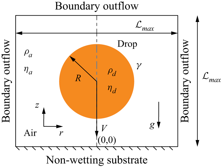
We employ direct numerical simulations to study the drop impact process in an axisymmetric setting (figure 1), using the free software program Basilisk C (Popinet Reference Popinet2013–2022a) that employs the geometric volume of fluid (VoF) method for interface reconstruction (Popinet Reference Popinet2009). For an incompressible flow, the mass conservation requires the velocity field to be divergence free (tildes denote dimensionless quantities throughout this manuscript):
 \begin{equation} \tilde{\boldsymbol{\nabla}}\boldsymbol{\cdot} \tilde{\boldsymbol{v}} = 0, \end{equation}
where we non-dimensionalise the velocity field with the inertio-capillary velocity  $V_\gamma = \sqrt {\gamma /(\rho _d R)}$. We further non-dimensionalise all lengths with the drop radius
 $R$ (figure 1), time with the inertio-capillary time scale,
 $\tau = \sqrt {\rho _dR^3/\gamma } = R/V_\gamma$, and pressure with the capillary pressure,
 $p_\gamma = \gamma /R$, to write the momentum equation as
 \begin{equation} \frac{\partial \tilde{\boldsymbol{v}}}{\partial \tilde{t}} + \boldsymbol{\nabla} \boldsymbol{\cdot}(\tilde{\boldsymbol{v}} \tilde{\boldsymbol{v}}) = \frac{1}{\tilde{\rho}}(-\tilde{\boldsymbol{\nabla}} \tilde{p}^{\prime} + \tilde{\boldsymbol{\nabla}}\boldsymbol{\cdot} (2Oh\tilde{\boldsymbol{\mathcal{D}}}) + \tilde{\boldsymbol{f}}), \end{equation}
where the deformation tensor  $\boldsymbol {\mathcal {D}}$ is the symmetric part of the velocity gradient tensor
 $(= (\boldsymbol {\nabla }\boldsymbol {v} + (\boldsymbol {\nabla }\boldsymbol {v})^{T})/2)$. The Ohnesorge number
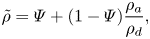
 $Oh$ (the ratio of inertio-capillary to inertio-viscous time scales) and the dimensionless density
 $\tilde {\rho }$ are written using the one-fluid approximation (Prosperetti & Tryggvason Reference Prosperetti and Tryggvason2009; Tryggvason, Scardovelli & Zaleski Reference Tryggvason, Scardovelli and Zaleski2011) as
 \begin{gather} Oh = \varPsi Oh_d + (1-\varPsi ){Oh}_{a}, \end{gather}
 \begin{gather}\tilde{\rho} = \varPsi + (1-\varPsi ) \frac{\rho_a}{\rho_d}, \end{gather}
where  $\varPsi$ is the VoF tracer (
 $= 1$ for the drop and
 $0$ otherwise), and
 $\rho _a/\rho _d$ is the air–drop density ratio. Here,
 \begin{equation} Oh_d = \frac{\eta_d}{\sqrt{\rho_d\gamma R}} \quad \text{and} \quad {Oh}_{a} = \frac{\eta_a}{\sqrt{\rho_d\gamma R}} \end{equation}
are the Ohnesorge numbers based on the viscosities of the drop liquid and of air, respectively. To minimise the influence of the surrounding medium, we keep  $\rho _a/\rho _d$ and
 ${Oh}_{a}$ fixed at
 $10^{-3}$ and
 $10^{-5}$, respectively. For a lean notation, we will use
 $Oh$ instead of
 $Oh_d$ in the remainder of the text.
Axisymmetric computational domain used to study the impact of a drop with radius  $R$ and velocity
 $V$ on an ideal non-wetting substrate. The subscripts
 $d$ and
 $a$ denote the drop and air, respectively, to distinguish their material properties, the density
 $\rho$ and viscosity
 $\eta$. The drop–air surface tension coefficient is
 $\gamma$ and
 $g$ denotes the acceleration due to gravity. The grey dashed-dotted line represents the axis of symmetry,
 $r = 0$. Boundary outflow is applied at the top and side boundaries (tangential stresses, normal velocity gradient and ambient pressure are set to zero). The domain boundaries are far enough not to influence the drop impact process (
 $\mathcal {L}_{max} \gg R$,
 $\mathcal {L}_{max} = 8R$ in the worst case).
Lastly,  $\tilde {p}^{\prime }$ denotes the reduced pressure field,
 $\tilde {p}' = \tilde {p}\,+\,Bo\tilde {\rho }\tilde {z}$, where
 $\tilde {p}$ and
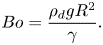
 $Bo\tilde {\rho }\tilde {z}$ represent the mechanical and the hydrostatic pressures, respectively. Here,
 $\tilde {z}$ is the distance away from the non-wetting substrate (see figure 1) and the Bond number
 $Bo$ compares gravity with the surface tension force
 \begin{equation} Bo = \frac{\rho_d g R^2}{\gamma}. \end{equation}
Using this reduced pressure approach ensures an exact hydrostatic balance as described in Popinet (Reference Popinet2018) and Popinet et al. Reference Popinet(2013–2022b). This formulation requires an additional singular body force at the interface such that  $\tilde {\boldsymbol {f}}$ takes the form (Brackbill, Kothe & Zemach Reference Brackbill, Kothe and Zemach1992)
 \begin{equation} \tilde{\boldsymbol{f}} \approx \left(\tilde{\kappa} + Bo\left(1 -\frac{\rho_a}{\rho_d}\right)\tilde{z}\right) \tilde{\boldsymbol{\nabla}}\varPsi, \end{equation}
where the first and second terms on the right-hand side are the local capillary and hydrostatic pressure jumps across the interface, respectively, with  $\tilde {\kappa }$ the interfacial curvature calculated using the height-function approach (Popinet Reference Popinet2009).
Figure 1 shows the axisymmetric computational domain where we solve the equations discussed above. A no-slip and no-penetration boundary condition is applied on the substrate along with a zero normal pressure gradient. Here, we also impose  $\varPsi = 0$ to maintain a thin air layer between the drop and the substrate to model an ideal non-wetting substrate (for a detailed discussion about this method, readers are referred to Sanjay Reference Sanjay2022b). Physically, this implies that the minimum thickness of this air layer is
 $\varDelta /2$, where
 $\varDelta$ is the minimum grid size, throughout the simulation duration. We use Basilisk C's (Popinet Reference Popinet2013–2022a) adaptive mesh refinement capabilities to finely resolve regions of high velocity gradients and at the drop–air interface. We undertook a mesh independence study to ensure that the results are independent of this mesh resolution and use a minimum grid size
 $\varDelta = R/1024$ for this study. Initially, we assume that the drop is spherical and that it impacts with a dimensionless velocity,
 $\tilde {V} = V/V_\gamma = \sqrt {We}$, where the impact Weber number
 \begin{equation} We = \frac{\rho_d R V^2}{\gamma}, \end{equation}
is the ratio of the inertial pressure during impact to the capillary pressure. We refer the readers to Popinet (Reference Popinet2009, Reference Popinet2015, Reference Popinet2013–2022a), Zhang et al. (Reference Zhang, Sanjay, Shi, Zhao, Lv and Lohse2022) and Sanjay (Reference Sanjay2022a,Reference Sanjayb) for details of the computational method employed in this work.
3. Bouncing inhibition
We investigate the behaviour of drops impacting on non-wetting substrates by exploring the influence of the following dimensionless parameters: the Weber number  $We = \rho R V^2/\gamma$, the Bond number
 $Bo = \rho _dgR^2/\gamma$ and the drop Ohnesorge number
 $Oh = \eta _d/\sqrt {\rho _d\gamma R}$. We restrict ourselves to impacts with
 $We \ge 1$ and do not discuss the bouncing to non-bouncing transition observed for
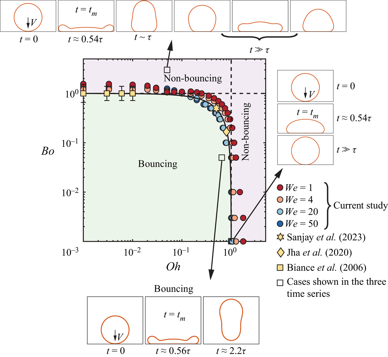
 $We \ll 1$ (gentle deposition) (Richard & Quéré Reference Richard and Quéré2000; Moláček & Bush Reference Moláček and Bush2012; Planchette, Biance & Lorenceau Reference Planchette, Biance and Lorenceau2012). In figure 2, we evidence the bouncing to non-bouncing transition in the parameter space spanned by the Ohnesorge and Bond numbers for several fixed Weber numbers. We extract three key pieces of information from this regime map:
(i) The Weber number has a small influence on the transition between the bouncing and non-bouncing regime in the range probed in this study,
 $We = 1\unicode{x2013}50$, the same as what was reported by Jha et al. (Reference Jha, Chantelot, Clanet and Quéré2020) and Antonini et al. (Reference Antonini, Jung, Wetzel, Heer, Schoch, Moqaddam, Chikatamarla, Karlin, Marengo and Poulikakos2016) for the bouncing inhibition of viscous drops (see also Appendix B).
(ii) We recover the two limiting cases of non-bouncing (see insets of figure 2): drops smaller than their visco-capillary length, (i.e.
$R < \eta _d^2/\rho _d\gamma$, giving $Oh > 1$) stop bouncing due to viscous dissipation (Jha et al. Reference Jha, Chantelot, Clanet and Quéré2020), while those larger than their gravito-capillary length, (i.e. $R > \sqrt {\gamma /\rho _d g}$, giving $Bo > 1$) cannot bounce due to their weight (Biance et al. Reference Biance, Chevy, Clanet, Lagubeau and Quéré2006). We will elaborate on the mechanisms of rebound inhibition in these two non-bouncing regimes in § 4.(iii) Experiments performed with millimetre-sized drops of water or silicone oil do not lie on either asymptote (Jha et al. Reference Jha, Chantelot, Clanet and Quéré2020; Sanjay et al. Reference Sanjay, Lakshman, Chantelot, Snoeijer and Lohse2023), suggesting that both the effects of viscosity and gravity need to be taken into account to predict the bouncing to non-bouncing transition.


Regime map in terms of the Bond number  $Bo = \rho _dgR^2/\gamma$ and the drop Ohnesorge number
 $Oh = \eta _d/\sqrt {\rho _d\gamma R}$, distinguishing the bouncing and non-bouncing regimes. The data points represent the transition between the bouncing and non-bouncing regimes at different Weber numbers
 $We$. The three series of insets illustrate typical cases in these regimes, namely
 $(We, Oh, Bo) = (16, 0.05, 3)$ for the upper,
 $(16, 1, 0.001)$ for the right and
 $(16, 0.75, 0.05)$ for the bottom series of images, respectively. The solid black line delineates the prediction of this transition ((3.6)). Lastly, the black dashed vertical and horizontal lines mark the two asymptotes, i.e. the viscous limiting case,
 ${Oh}_{c} = 1$ and the weight limiting case,
 ${Bo}_{c} = 1$, respectively. See also the supplementary movie SM1 available at https://doi.org/10.1017/jfm.2023.55.
In this section, we focus on situations where bouncing is prevented by both viscous and gravitational effects (i.e.  $Bo < 1$ and
 $Oh < 1$). Figure 3 shows snapshots illustrating three representative cases lying in this region of the parameter space for
 $We = 20$. Each snapshot displays three pieces of information: the position of the liquid–air interface, the dimensionless rate of viscous dissipation per unit volume (i.e. the dimensionless viscous dissipation function, left panel) and the magnitude of the velocity field normalised with the initial impact velocity (right panel). For
 $Oh = 0.2$ and
 $Bo = 0.4$ (figure 3a), the drop undergoes typical rebound dynamics. The liquid first spreads radially up to
 $t = t_m$, when the maximum extent is reached (Clanet et al. Reference Clanet, Béguin, Richard and Quéré2004; Eggers et al. Reference Eggers, Fontelos, Josserand and Zaleski2010; Laan et al. Reference Laan, de Bruin, Bartolo, Josserand and Bonn2014; Wildeman et al. Reference Wildeman, Visser, Sun and Lohse2016). This stage is followed by liquid retraction (Bartolo et al. Reference Bartolo, Josserand and Bonn2005), parallel to the substrate, until the drop contracts (
 $t = 2t_m$) and the motion becomes vertical (Chantelot Reference Chantelot2018; Zhang et al. Reference Zhang, Sanjay, Shi, Zhao, Lv and Lohse2022). Finally, the drop leaves the substrate at
 $t = 2.25\tau$ (Richard & Quéré Reference Richard and Quéré2000; Richard et al. Reference Richard, Clanet and Quéré2002).
Direct numerical simulations snapshots illustrating the drop impact dynamics for (a)  $(Oh, Bo) = (0.2, 0.4)$, (b)
 $(Oh, Bo) = (0.6, 0.4)$ and (c)
 $(Oh, Bo) = (0.2, 0.8)$. The left-hand side of each numerical snapshot shows the dimensionless viscous dissipation function
 $\tilde {\xi }_\eta = 2Oh(\tilde {\boldsymbol{\mathcal{D}}}:\tilde {\boldsymbol{\mathcal{D}}})$ on a
 $\log _{10}$ scale to identify regions of maximum dissipation (black). The right-hand side shows the magnitude of the velocity field normalised by the initial impact velocity,
 $V$. The black velocity vectors are plotted in the drop's centre of mass reference frame to evidence the internal flow. The numbers inside the bracket at right-top corner of each snapshot represent the dimensionless time,
 $t/\tau$. For all cases, the impact Weber number is
 $We = 20$. See also the supplementary movie SM2.
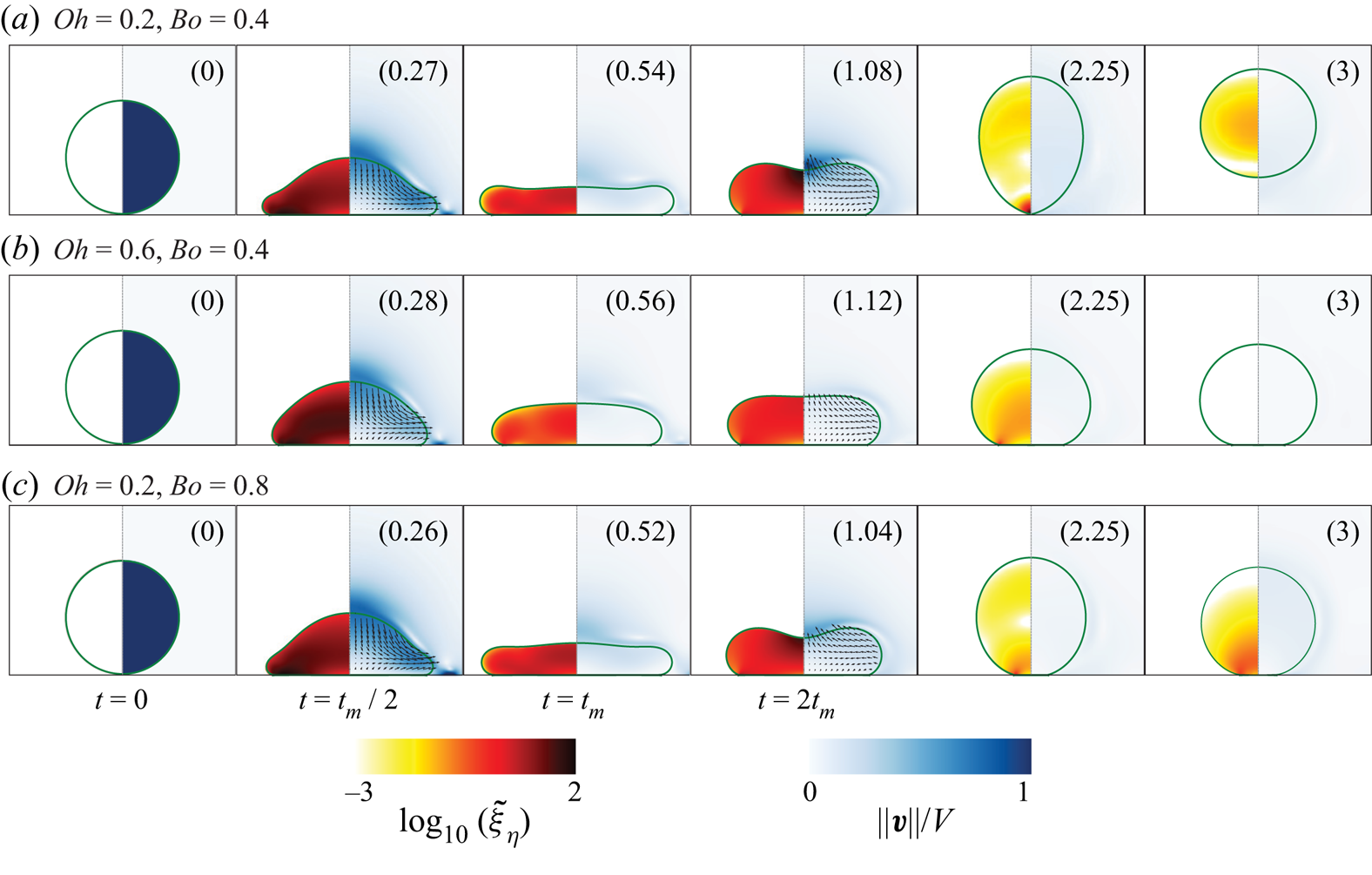
Surprisingly, increasing  $Oh$ to
 $0.6$, below the critical value reported by Jha et al. (Reference Jha, Chantelot, Clanet and Quéré2020), while keeping
 $Bo = 0.4$ (figure 3b), prevents the rebound. The motion is damped before the drop can bounce off the substrate. Similarly, increasing
 $Bo$ to 0.8, below the critical value reported by Biance et al. (Reference Biance, Chevy, Clanet, Lagubeau and Quéré2006), while fixing
 $Oh = 0.2$ (figure 3c), also inhibits bouncing. Yet, the deposited liquid undergoes multiple oscillation cycles on the substrate before coming to rest (see the last snapshot
 $t = 3\tau$).
In all three cases, the impact dynamics and flow in the drop are qualitatively similar until the maximum extent is reached at  $t=t_m$. At this instant, the absence of internal flow suggests that the initial kinetic energy has either been converted into surface energy or lost to viscous dissipation, which occurs throughout the drop volume owing to
 $Oh \sim {O}(0.1)$ (Eggers et al. Reference Eggers, Fontelos, Josserand and Zaleski2010). Close to the bouncing to non-bouncing transition, the rebound can thus be understood as a process which converts an initial surface energy into kinetic energy, disentangling the later stages of the rebound from the initial impact dynamics.
This observation prompts us to introduce an analogy with coalescence-induced jumping, in which an excess surface energy, gained during coalescence, is converted into upward motion of the liquid (Boreyko & Chen Reference Boreyko and Chen2009; Liu et al. Reference Liu, Ghigliotti, Feng and Chen2014; Farokhirad et al. Reference Farokhirad, Morris and Lee2015). The spread drop, at rest at  $t=t_m$, reduces its surface area through a Taylor–Culick-type retraction, converting excess surface energy into kinetic energy. The capillary force driving this radially inwards flow is
 \begin{equation} F_\gamma \sim \gamma R. \end{equation}
The velocity  $v$ associated with this Taylor–Culick-type retraction scales as
 $v \sim \sqrt {\gamma /(\rho _d e)}$, where
 $e$ is the typical thickness of the spread liquid, which can be rearranged as
 $v \sim V_\gamma \sqrt {R/e}$ upon introducing the inertio-capillary velocity (Bartolo et al. Reference Bartolo, Josserand and Bonn2005; Chantelot Reference Chantelot2018). At the bouncing to non-bouncing transition, in the presence of both viscous and gravitational effects (see figure 2), we make the hypothesis that
 $e \sim R$, as no pronounced central film forms during spreading (see figure 3 at
 $t=t_m$), implying that the inertio-capillary velocity is the relevant velocity scale, i.e.
 $v \sim V_\gamma$. Similarly to the coalescence-induced jumping of two identical drops, a dissipative force
 $F_\eta \sim \varOmega \eta _d\nabla ^2v$, where
 $\varOmega$ is the volume of the drop and
 $v$ is a typical radial flow velocity, opposes the capillarity driven flow (Mouterde et al. Reference Mouterde, Nguyen, Takahashi, Clanet, Shimoyama and Quéré2017b; Lecointre et al. Reference Lecointre, Mouterde, Checco, Black, Rahman, Clanet and Quéré2019). Taking
 $v \sim V_\gamma$ as explained above, the resistive viscous force then scales as
 \begin{equation} F_\eta \sim \eta_d V_\gamma R, \end{equation}
and the effective momentum converging in the radial direction is
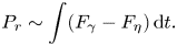 \begin{equation} P_r \sim \int (F_\gamma - F_\eta)\, \mathrm{d}t. \end{equation}
The asymmetry originating from the presence of the substrate enables the conversion of the radially inward momentum to the upwards direction (figure 3,  $t = 2t_m$). Following Mouterde et al. (Reference Mouterde, Nguyen, Takahashi, Clanet, Shimoyama and Quéré2017b) and Lecointre et al. (Reference Lecointre, Mouterde, Checco, Black, Rahman, Clanet and Quéré2019), we assume that the vertical momentum scales with the radial one, i.e.
 $P_v \sim P_r$, allowing us to determine a criterion for the bouncing transition by balancing the rate of change of vertical momentum with the drop's weight
 $F_g$:
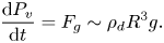 \begin{equation} \frac{{\rm d} P_v}{{\rm d} t} = F_g \sim \rho_d R^3 g. \end{equation}
 \begin{equation} \gamma R - \eta_d V_\gamma R \sim \rho_dR^3g. \end{equation}
Lastly, substituting  $V_\gamma = \sqrt {\gamma /\rho _dR}$, and rearranging, we arrive at a criterion to determine the bouncing to non-bouncing transition as
 \begin{equation} {Oh}_{c} + {Bo}_{c} \sim 1, \end{equation}
where the subscript  $c$ stands for ‘critical’. Equation (3.6), which is independent of the impact Weber number
 $We$, is the main result of the manuscript.
We test the criterion (3.6) for the bouncing to floating transition against data extracted from our direct numerical simulations and experiments from Biance et al. (Reference Biance, Chevy, Clanet, Lagubeau and Quéré2006), Jha et al. (Reference Jha, Chantelot, Clanet and Quéré2020) and Sanjay et al. (Reference Sanjay, Lakshman, Chantelot, Snoeijer and Lohse2023). In figure 2, the solid black line, representing (3.6) with prefactor  $1$, is in excellent quantitative agreement with the data when viscous and gravitational effects inhibit bouncing, as well as in the two limiting regimes,
 ${Oh}_{c} \sim 1$ for
 $Bo \ll 1$ (Jha et al. Reference Jha, Chantelot, Clanet and Quéré2020), and
 ${Bo}_{c} \sim 1$ for
 $Oh \ll 1$ (Biance et al. Reference Biance, Chevy, Clanet, Lagubeau and Quéré2006) (black dotted lines).
In the next section, we focus on evidencing the physical mechanisms leading to bouncing suppression in each of the two limiting cases. But before this, we note that the data for different Weber numbers do not exactly collapse on the prediction of (3.6), suggesting that the critical Ohnesorge and Bond numbers vary weakly with the Weber number, and hinting at the limitations of our hypothesis in choosing  $V_\gamma$ as the velocity scale, and neglecting the influence of
 $We$ on the retraction velocity.
4. Limiting cases
4.1. How does a viscous drop stop bouncing?
We first investigate how viscous drops, much smaller than their gravito-capillary length, i.e. with  $Bo \ll 1$, stop bouncing. We study this regime, in which the transition criterion (3.6) reduces to
 ${Oh}_{c} \sim 1$, by setting
 $Bo$ to
 $0$ (i.e. by assuming that capillarity dominates over gravity) and by systematically varying the drop Ohnesorge number,
 $Oh$. We characterise the rebound behaviour by measuring the apparent contact time
 $t_c$ between the drop and the substrate and the coefficient of restitution
 $\varepsilon$, that we define as
 $\varepsilon = v_{cm}(t_c)/V$, where
 $v_{cm}(t_c)$ is the centre of mass velocity at take-off. The procedure used to extract
 $t_c$ and
 $\varepsilon$ from the direct numerical simulations is detailed in Appendix A.
In figure 4, we plot the coefficient of restitution  $\varepsilon$ and the normalised contact time
 $t_c/\tau$ as a function of
 $Oh$ for Weber numbers ranging from 1 to 50. The effect of
 $Oh$ on
 $\varepsilon$ and
 $t_c$ is markedly different. On the one hand, the coefficient of restitution monotonically decreases from its low
 $Oh$, Weber-dependent value
 \begin{equation} \varepsilon_0(We) = \varepsilon(We, Oh \to 0, Bo = 0), \end{equation}
with increasing  $Oh$, until a critical Ohnesorge number of order one,
 ${Oh}_{c}$, marking the end of the bouncing regime. On the other hand, increasing
 $Oh$ by over two orders of magnitude hardly affects
 $t_c$. It keeps its Weber-independent value
 $\tau _0 = 2.25\tau$, expected from the inertio-capillary scaling in the low
 $Oh$ limit (Wachters & Westerling Reference Wachters and Westerling1966; Richard et al. Reference Richard, Clanet and Quéré2002), until
 $t_c$ diverges as
 $Oh$ tends towards
 ${Oh}_{c}$.
Variation of (a) the restitution coefficient  $\varepsilon$, and (b) the contact time
 $t_c$, normalised by the inertio-capillary time scale
 $\tau = \sqrt {\rho _dR^3/\gamma }$, with the drop Ohnesorge number
 $Oh$ for
 $Bo = 0$ at different Weber numbers
 $We$. In both panels, the solid lines represent the predictions of the spring–mass–damper system of Jha et al. (Reference Jha, Chantelot, Clanet and Quéré2020) (contact time, (4.3) and restitution coefficient, (4.4)). The horizontal dashed lines represent the contact time and restitution coefficient values in the
 $Oh \ll 1$ limit, in which
 $\tau _0 = 2.25\tau$, independent of
 $We$, while
 $\varepsilon _0(We) = \varepsilon (We, Oh \to 0, Bo = 0)$ (4.1) depends on
 $We$. Lastly, the black vertical lines and the grey shaded regions mark the critical Ohnesorge number
 ${Oh}_{c} \sim {O}(1)$ beyond which drops do not bounce.
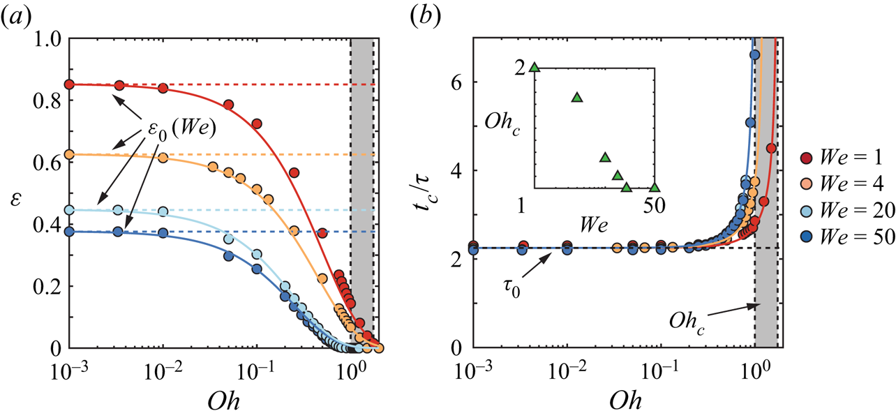
Figure 4 also highlights that  ${Oh}_{c}$ varies weakly with
 $We$ (
 ${Oh}_{c} = 1.75, 1.5, 1, 1$ at
 $We = 1, 4, 20, 50$, respectively, see inset of figure 4b) as evidenced by the narrow grey shaded region, and in agreement with the limit predicted from (3.6). Varying
 $We$ mainly affects the low
 $Oh$ restitution limit
 $\varepsilon _0(We)$, which we elaborate on in Appendix B. We stress that the weak variation of the coefficient of restitution in the shaded region, where
 $\varepsilon <0.1$, could go unnoticed in typical side view experiments. Indeed,
 $\varepsilon = 0.1$ corresponds to a centre of mass rebound height of
 $0.01$ times the initial impact height, that is
 $10\ \mathrm {\mu }{\rm m}$ for
 $We = 1$.
We now seek to understand the evolution of the restitution coefficient  $\varepsilon$ with
 $Oh$ by quantifying the overall energy budget during an impact event. In the
 $Bo = 0$ limit, the energy balance reads
 \begin{equation} \tilde{E}_0 = \tilde{E}_k(\tilde{t}) + {\rm \Delta}\tilde{E}_\gamma(\tilde{t}) + \tilde{E}_\eta(\tilde{t}), \end{equation}
where each energy component is normalised using the capillary energy scale  $\gamma R^2$,
 $E_0$ denotes the drop's initial kinetic energy, (
 $\tilde {E}_0 = E_0/(\gamma R^2) = (2{\rm \pi} /3)We$),
 $E_k(t)$ and
 $E_\gamma (t)$ are the drop's time-dependent kinetic and surface energies, with
 ${\rm \Delta} E_\gamma (t) = E_\gamma (t) - E_\gamma (t = 0)$, and
 $E_\eta (t)$ is the viscous dissipation until time
 $t$. Readers are referred to Landau & Lifshitz (Reference Landau and Lifshitz1987), Wildeman et al. (Reference Wildeman, Visser, Sun and Lohse2016), Ramírez-Soto et al. (Reference Ramírez-Soto, Sanjay, Lohse, Pham and Vollmer2020), Sanjay et al. (Reference Sanjay, Sen, Kant and Lohse2022b) and Sanjay (Reference Sanjay2022) for details of energy budget calculations.
Figure 5(a) evidences the time evolution of the energy balance contributions for an impact with  $We=1$ and
 $Oh=0.001$. The drop's initial kinetic energy
 $E_0$ is transferred into surface energy until the liquid reaches its maximal extent at
 $t = t_m$ (note that for
 $We = 1$,
 $t_m \approx \tau$, see Zhang et al. Reference Zhang, Sanjay, Shi, Zhao, Lv and Lohse2022). At this instant, the energy available to the drop is almost exclusively stored in the form of excess surface energy, as hypothesised in our analogy with coalescence-induced jumping. As the drop retracts, surface energy is converted back into kinetic energy and, at take-off, the drop recovers a large proportion of its initial kinetic energy,
 $E_k(t_c) \approx 0.75E_0$. Energy dissipation throughout the rebound,
 $E_\eta (t_c)$, and the non-spherical drop shape at take-off, storing excess surface energy
 ${\rm \Delta} E_\gamma (t_c)$, hamper the recovery of the initial kinetic energy. Even in the low
 $We$ and low
 $Oh$ case at hand, where dissipation is restricted to the boundary layer at the drop–air interface and happens due to the propagation of capillary waves (see the insets of figure 5(a) and Renardy et al. Reference Renardy, Popinet, Duchemin, Renardy, Zaleski, Josserand, Drumright-Clarke, Richard, Clanet and Quéré2003; Zhang et al. Reference Zhang, Sanjay, Shi, Zhao, Lv and Lohse2022), viscous stresses dissipate
 $20$% of the initial energy during the rebound.
Energy budgets for drop impacts with  $Bo = 0$ and
 $We = 1$ for (a)
 $Oh = 0.001$ and (b)
 $Oh = 2$. Here,
 $E_k$ and
 $E_\eta$ represent the kinetic energy and viscous dissipation, respectively,
 ${\rm \Delta} E_\gamma$ denotes the change in surface energy with its zero set at
 $t = 0$. The numerical snapshots in the insets illustrate the drop morphologies and the anatomy of the flow with a colour code identical to that of figure 3. The black dotted lines in panels (a) and (b) mark the instant
 $t_c$ when the drop takes off and when the normal contact force between the drop and the substrate is minimum, respectively. (c,d) Energy distributions at
 $t = t_c$ for
 $We = 1$ (c) and
 $We = 20$ (d) as function of
 $Oh$. The black vertical lines and the grey shaded regions mark the critical Ohnesorge number
 ${Oh}_{c} \sim {O}(1)$ beyond which drops do not bounce. See also supplementary movie SM3.
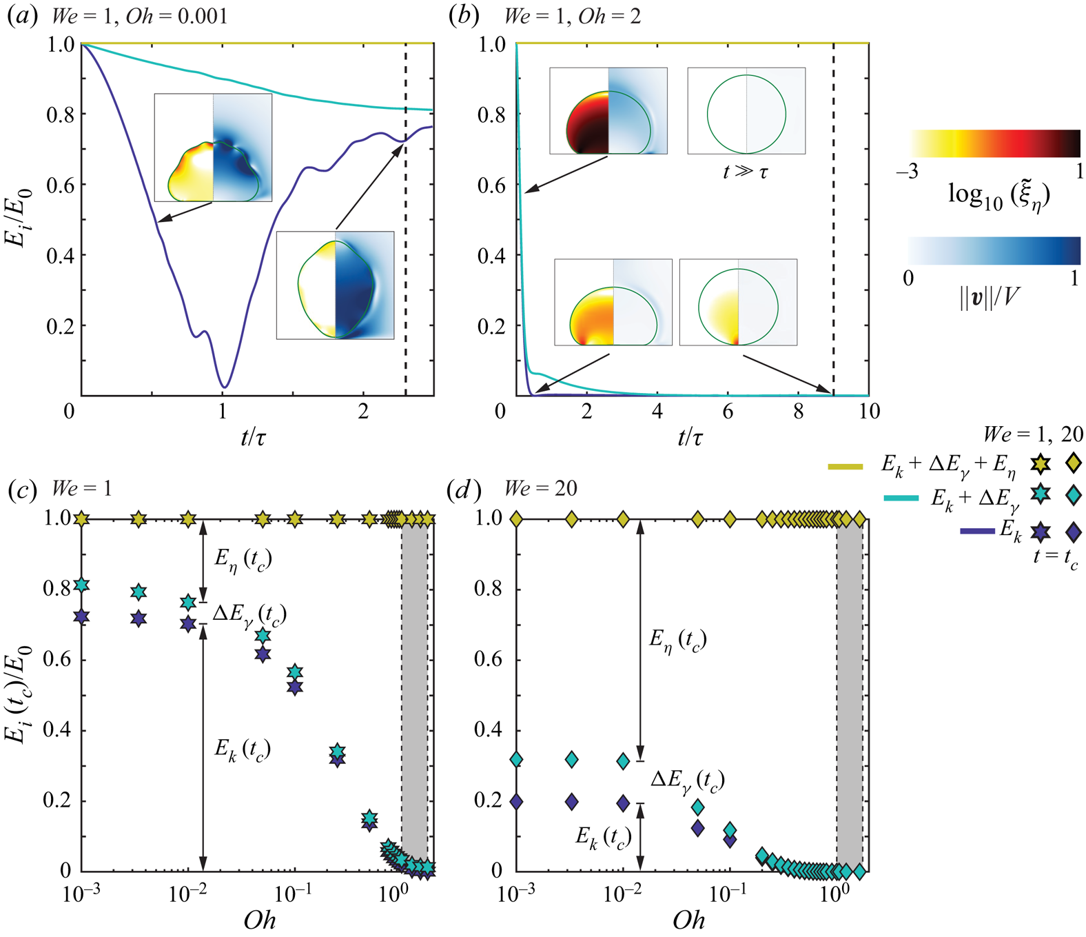
Increasing the drop Ohnesorge number to  $Oh = 2$ does not affect the energy transfer dynamics (figure 5b), but it enhances viscous dissipation, which now takes place in the whole liquid volume (see the insets of figure 5(b) and Eggers et al. Reference Eggers, Fontelos, Josserand and Zaleski2010). Beyond the critical Ohnesorge number
 ${Oh}_{c}$, the initial kinetic energy is dissipated before the drop can rebound off the substrate. The drop impact process becomes over-damped and, in this small Bond number limit, the drop slowly relaxes back to its sessile spherical shape (figure 5b).
Figures 5(c) and (d) summarise the distribution of energy at take-off as a function of  $Oh$ for
 $We = 1$ and
 $We = 20$, respectively. For
 $Oh < 0.01$, the overall energy budget is not affected by a change in drop Ohnesorge number, extending the validity domain of the so-called inviscid drop limit (Richard & Quéré Reference Richard and Quéré2000). Strikingly, the independence of
 $E_\eta (t_c)$, and thus of
 $\varepsilon$, with
 $Oh$ in this limit does not imply that viscous dissipation is negligible. Indeed, (i) the dissipated energy accounts for more than two thirds of the total kinetic energy loss during impact at
 $We = 1$, where the restitution is maximal, and (ii) the increase of viscous dissipation is mainly responsible for the decrease of
 $\varepsilon$ with
 $We$. The dissipated energy
 $E_\eta (t_c)$ accounts for
 $20\,\%$ and
 $70\,\%$ of
 $E_0$ for
 $We = 1$ and
 $We = 20$, respectively, contradicting the inviscid nature of this regime. The transfer of the initial kinetic energy into surface energy
 ${\rm \Delta} E_\gamma (t_c)$ at take-off, that is the rebound of the liquid in a non-spherical shape, while accounting for one third the total energy loss during impact at
 $We = 1$, cannot alone explain the significantly lower than one value of the coefficient of restitution.
The presence of a finite energy dissipation in the limit  $Oh \to 0$ is reminiscent of the dissipative anomaly in fully developed turbulence, expressing that, even in the limit of vanishing viscosity (i.e. diverging Reynolds number
 $Re \to \infty$), the energy dissipation rate remains finite (Kolmogorov Reference Kolmogorov1941; Onsager Reference Onsager1949; Eyink Reference Eyink1994; Eggers Reference Eggers2018; Dubrulle Reference Dubrulle2019). The dissipative anomaly reflects in the finite drag experienced by solid bodies at diverging Reynolds numbers, through the creation of boundary layers (Prandtl Reference Prandtl1904), somewhat similar to the localisation of viscous dissipation at the liquid–air interface during drop impact (see the inset of figure 5(a) and Philippi et al. Reference Philippi, Lagrée and Antkowiak2016).
For larger Ohnesorge numbers, the dissipated energy  $E_\eta (t_c)$ increases with
 $Oh$, reflecting that viscous dissipation is responsible for the loss of the rebound elasticity. Interestingly, increasing
 $Oh$ also reduces the drop deformation at take-off, decreasing the fraction of energy stored as surface energy
 ${\rm \Delta} E_\gamma (t_c)$. Consequently, energy which is not lost to viscous dissipation is mainly converted back into the kinetic energy of the drop, leading to a more efficient recovery of the initial kinetic energy (figure 5c,d).
We further rationalise our observations by comparing our simulation results with the predictions of Jha et al. (Reference Jha, Chantelot, Clanet and Quéré2020) that extend the liquid spring analogy to viscous drops. This minimal model, that has been shown to successfully capture the variation of  $t_c$ and
 $\varepsilon$ with
 $Oh$, gives the time of apparent contact as
 \begin{equation} t_c(We,Oh, Bo = 0) = \tau_0 \left(\frac{1}{\sqrt{1 - (Oh/{Oh}_{c} (We))^{2}}}\right), \end{equation}
which is in quantitative agreement with our simulation data (figure 4b) when the critical Ohnesorge number  ${Oh}_{c}(We)$ at which bouncing stops is taken from the simulations (see the inset of figure 4b). Jha et al. (Reference Jha, Chantelot, Clanet and Quéré2020) also predict the coefficient of restitution, written in our notations as
 \begin{equation} \varepsilon(We, Oh, Bo = 0) = \varepsilon_0(We)\exp\left( \frac{-\beta Oh/{Oh}_{c}(We)}{\sqrt{1 - (Oh/{Oh}_{c}(We))^{2}}} \right), \end{equation}
where  $\beta$ is an adjustable
 $We$-independent parameter. The simulation data and the model are in excellent agreement for
 $\beta = 4.00 \pm 0.25$ (figure 4a). Note that Jha et al. (Reference Jha, Chantelot, Clanet and Quéré2020) further reduced (4.4) to
 $\varepsilon (We, Oh, Bo = 0) \approx \varepsilon _0(We)\exp (-\alpha Oh )$ for
 $Oh \ll {Oh}_{c}$, where
 $\alpha = \beta /{Oh}_{c} = 2.5 \pm 0.5$ best fits the experimental data, independent of the impact Weber number. The equivalent fitting parameter for our case is
 $\alpha ^{\prime } = \beta ^\prime /{Oh}_{c} = 3 \pm 1$, in very good agreement with the value reported by Jha et al. (Reference Jha, Chantelot, Clanet and Quéré2020), despite the different Bond number (
 $Bo = 0$ here vs.
 $Bo = 0.167$ for Jha et al. (Reference Jha, Chantelot, Clanet and Quéré2020), also see § 4.2 and Appendix B).
Finally, we discuss the failure of the model of Jha et al. (Reference Jha, Chantelot, Clanet and Quéré2020) to predict the low  $Oh$ behaviour of the coefficient of restitution that is contained in the prefactor
 $\varepsilon _0$. The analysis of the overall energy budget shows that two ingredients are responsible for the loss of the initial drop kinetic energy in the
 $Oh < 0.01$ limit: (i) the presence of excess surface energy at take-off
 ${\rm \Delta} E_\gamma (t_c)$ and (ii) the viscous dissipation in thin boundary layers at the liquid–air interface. Both these contributions are not accounted for in the model of Jha et al. (Reference Jha, Chantelot, Clanet and Quéré2020) which takes no deformation, i.e.
 ${\rm \Delta} E_\gamma (t_c) = 0$ as a take-off condition, and
 $\eta _d V R$ as the scaling form of the viscous damping term, added to the liquid spring, which supposes that dissipation occurs at the drop length scale. However, as
 $Oh$ increases, bulk dissipation becomes dominant, explaining the ability of the model to capture bouncing inhibition.
4.2. How does a heavy drop stop bouncing?
We now discuss the rebound inhibition of heavy drops, much larger than than their visco-capillary lengths, i.e. with  $Oh \ll 1$. We study this limit, in which (3.6) reduces to
 ${Bo}_{c} \sim 1$, by fixing
 $Oh = 0.01$, in the so-called inviscid bouncing regime (figures 4 and 5), and by varying the Bond number
 $Bo$.
In figure 6, we show the evolution of the coefficient of restitution  $\varepsilon$ and of the normalised contact time
 $t_c/\tau$ as a function of the Bond number
 $Bo$ for four values of the Weber number. The variation of
 $\varepsilon$ with
 $Bo$ is qualitatively similar to that observed when sweeping across the viscous drop asymptote. The coefficient of restitution
 $\varepsilon$ slowly decreases from its Weber-dependent value
 $\varepsilon _*(We) = \varepsilon (We,Oh = 0.01,Bo = 0)$ with increasing Bond number, until it approaches a critical Bond number
 ${Bo}_{c}$, of order one, at which it sharply decreases to zero. Here, in the so-called inviscid regime,
 $\varepsilon _*(We) \approx \varepsilon _0(We)$. However, the influences of
 $Bo$ and
 $Oh$ on
 $t_c$ are different. The contact time value hardly deviates from its inertio-capillary value,
 $\tau _0 = 2.25 \tau$, when varying
 $Bo$ over two orders of magnitude. Yet, we only observe a moderate increase of
 $t_c$ as
 ${Bo}_{c}$ is approached, contrasting with the divergence of
 $t_c$ close to
 ${Oh}_{c}$.
Variation of (a) the restitution coefficient  $\varepsilon$, and (b) the contact time
 $t_c$, normalised by the inertio-capillary time scale
 $\tau = \sqrt {\rho _dR^3/\gamma }$, with the Bond number
 $Bo$ at different Weber numbers
 $We$ in the so-called inviscid regime (
 $Oh = 0.01$). In panel (b), the solid lines represent the predictions of the model of Biance et al. (Reference Biance, Chevy, Clanet, Lagubeau and Quéré2006), see (4.6). The horizontal dashed lines represent the contact time and restitution coefficient values in the limit of zero Bond number (
 $\varepsilon (We, Oh = 0.01, Bo = 0)$), while the black vertical lines and the grey shaded regions mark the critical Bond number
 ${Bo}_{c} \sim {O}(1)$ beyond which drops do not bounce. Note that the model of Biance et al. (Reference Biance, Chevy, Clanet, Lagubeau and Quéré2006) predicts a constant
 $t_c$ (horizontal dashed line in panel a), in contradiction to our numerical simulations.

Figure 6 also evidences that varying the Weber number  $We$ from 1 to 50 hardly affects the critical Bond number
 ${Bo}_{c}$ (see the inset of figure 6b), marking the transition from bouncing to floating, as underlined by the grey shaded regions and in agreement with the transition criterion (3.6). Similarly as for viscous drops, increasing
 $We$ does not influence the contact time but markedly decreases
 $\varepsilon _*$, an effect we quantify in Appendix B.
To further investigate the variation of  $\varepsilon$ with
 $Bo$, we compute the overall energy budget during an impact event. In the presence of gravity, the energy balance (4.2) incorporates an additional contribution from the drop's gravitational potential energy,
 ${\rm \Delta} E_g$, whose zero is set at the instant of maximum drop deformation. The modified energy balance reads
 \begin{equation} \tilde{E}_0 = \tilde{E}_k(\tilde{t}) + {\rm \Delta}\tilde{E}_g(\tilde{t}) + {\rm \Delta}\tilde{E}_\gamma(\tilde{t}) + \tilde{E}_\eta(\tilde{t}), \end{equation}
where the initial energy also includes gravity,  $\tilde {E}_0 = (4{\rm \pi} /3)(We/2 + Bo(1-\mathcal {H}))$, with
 $\mathcal {H}$ denoting the centre of mass height of the drop at maximum deformation.
Figure 7(a) illustrates the energy budget for  $(We, Oh, Bo) = (1, 0.01,0)$. The energy transfer follows a similar dynamics as that described in figure 5(a), where
 $(We, Oh, Bo) = (1, 0.001, 0)$. The fraction of the initial kinetic energy recovered at take-off is the same,
 $E_k(t_c) \approx 0.75 E_0$. We also note that, although
 $Oh$ has increased by an order of magnitude compared with the case shown in figure 5(a), the energy lost to viscous dissipation still accounts for a similar fraction of the initial energy,
 $E_\eta (t_c)\approx 0.2 E_0$, as expected in the so-called inviscid drop limit. The snapshots of the drop's internal flow (see the insets of figures 5a and 7a) give insight into the independence of
 $E_\eta (t_c)$ with
 $Oh$. As the drop Ohnesorge number is increased, two antagonistic effects take place: (i) the viscous boundary layer grows larger, increasing dissipation, and (ii) capillary waves are attenuated, decreasing local dissipation. This competition qualitatively explains the independence of
 $E_\eta (t_c)$ and
 $\varepsilon$ on the drop Ohnesorge number for
 $Oh<0.01$.
Energy budgets for drop impacts with  $Oh = 0.01$ and
 $We = 1$ for
 $Bo = 0$ (a) and
 $Bo = 2$ (b). Here,
 $E_k$ and
 $E_\eta$ represent the kinetic energy and viscous dissipation, respectively,
 ${\rm \Delta} E_g$ and
 ${\rm \Delta} E_\gamma$ denote the the change in gravitational potential energy and surface energy with their zeros set at the instant of maximum spreading of the impacting drop, and at
 $t = 0$, respectively. The numerical snapshots in the insets illustrate the drop morphologies and the anatomy of the internal flow with a colour code identical to that of figure 3. The vertical dotted line in panel (a) marks the instant when the drop takes off. In panel (b), the black vertical lines and the grey shaded regions bounds the time interval when the normal contact force between the drop and the substrate is zero. (c,d) Energy distributions at
 $t = t_c$ for
 $We = 1$ (c) and
 $We = 20$ (d) as a function of
 $Bo$. For non-bouncing cases,
 $t_c$ represents the end of first drop oscillation cycle. The black vertical lines and the grey shaded regions in panels (c) and (d) mark the critical Bond number
 ${Bo}_{c} \sim {O}(1)$ beyond which drops do not bounce. See also supplementary movie SM4.
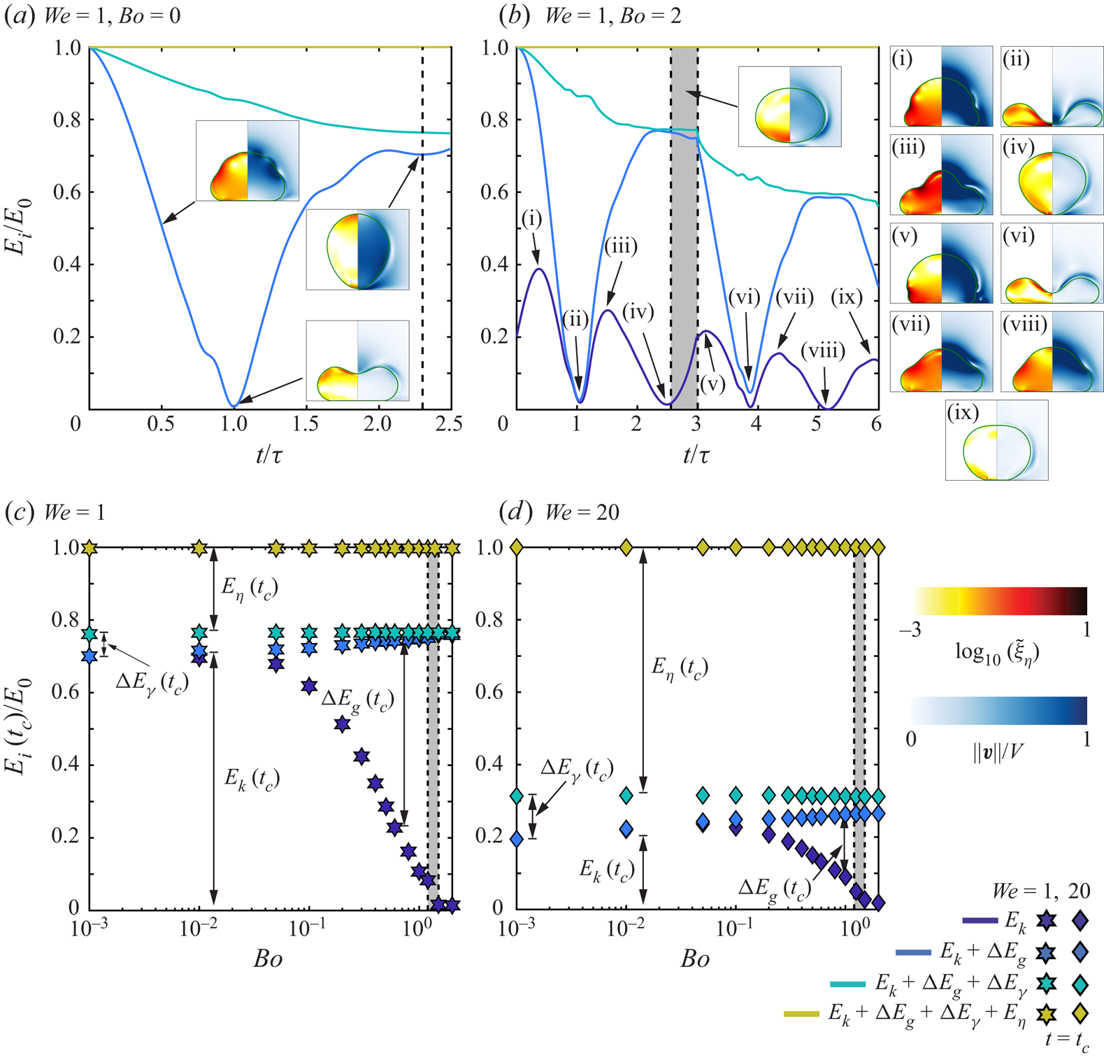
Increasing the Bond number to  $Bo = 2$, beyond
 ${Bo}_{c}$, sheds light on the mechanism of bouncing inhibition of heavy drops. At
 $t=0$, the drop has a higher initial energy owing to the contribution from the gravitational potential energy. As a result, the kinetic energy
 $E_k$ increases until the inertial shock is propagated throughout the drop (see figure 7b-i and Gordillo et al. Reference Gordillo, Sun and Cheng2018; Cheng, Sun & Gordillo Reference Cheng, Sun and Gordillo2021), before decreasing and reaching a minimum as the drop then attains maximum deformation (figure 7b-ii). In spite of these differences, the maximal spreading time is the same as that observed at low
 $Bo$,
 $t_m \approx \tau$ (for
 $We = 1$, see Zhang et al. Reference Zhang, Sanjay, Shi, Zhao, Lv and Lohse2022), and viscous dissipation enervates a similar proportion of the initial energy as in the low
 $Bo$ case during spreading. During the retraction stage,
 $E_k$ increases (figures 7b-ii to 7b-iii), until the motion goes from being dominantly in the radial direction to being dominantly in the axial direction (figure 7b-iii,
 $t \approx 1.5\tau$, see Chantelot Reference Chantelot2018; Zhang et al. Reference Zhang, Sanjay, Shi, Zhao, Lv and Lohse2022). Beyond this instant, gravity opposes the upward motion of the drop,
 $E_k$ decreases and is mainly transferred to
 $E_g$ until, eventually, at
 $t \approx 2.5\tau$ (figure 7b-iv) the drop's centre of mass starts moving in the downward direction. At this instant, only
 $20\,\%$ of the drop's initial energy goes to viscous dissipation, identical to the case of
 $Bo = 0$, but bouncing is inhibited. In contrast to the viscous asymptote, energy is still available to the drop even though the rebound is suppressed. Subsequently, the drop undergoes several capillary oscillations at the substrate with a time period of approximately
 $2.5\tau$ (figures 7b-v to 7b-ix).
Figures 7(c) and 7(d) show the distribution of energy at take-off as a function of  $Bo$ for
 $We = 1$ and
 $We =20$, respectively. For both Weber numbers, as
 $Bo$ increases, the fraction of initial energy that goes into viscous dissipation,
 $E_\eta (t_c)$, is constant. However, the gravitational potential energy
 ${\rm \Delta} E_g(t_c)$, initially negligible for
 $Bo = 0.001$, increases with increasing
 $Bo$, leading to a decrease of the drop's kinetic energy at take-off
 $E_k(t_c)$, which eventually drops to zero as bouncing stops at
 ${Bo}_{c}$. Noticing that energy is still available to the drop in the form of gravitational potential energy at
 $t=t_c$ allows us to rationalise the different behaviour of
 $t_c$ with
 $Bo$ and
 $Oh$. Indeed, the viscous rebound suppression corresponds to a transition from an underdamped to an overdamped system, associated with a divergence of the oscillation period, while heavy drops undergo successive energy transfers between gravitational potential, kinetic and surface energy on the inertio-capillary time scale.
Finally, we compare the variation of  $\varepsilon$ and
 $t_c$ with
 $Bo$ extracted from our simulations to the spring–mass model of Biance et al. (Reference Biance, Chevy, Clanet, Lagubeau and Quéré2006) which takes into account the role of gravity but neglects viscous dissipation. In our notation, the dependence of
 $\varepsilon$ on
 $Bo$ in the model of Biance et al. (Reference Biance, Chevy, Clanet, Lagubeau and Quéré2006) is written as
 \begin{equation} \varepsilon(We, Oh = 0.01, Bo) = \varepsilon_*(We)\sqrt{(1-Bo/{Bo}_{c}(We))(1 + Bo/(3{Bo}_{c}(We)))}. \end{equation}
Equation (4.6) is in excellent quantitative agreement with the values of  $\varepsilon _*(We)$ and
 ${Bo}_{c}(We)$ extracted from the simulations (figure 6a). However, this model predicts a constant
 $t_c$ which is in disagreement with our simulations as we approach
 $Bo_c$ (figure 6b). We further stress that the model of Biance et al. (Reference Biance, Chevy, Clanet, Lagubeau and Quéré2006), similarly to that of Jha et al. (Reference Jha, Chantelot, Clanet and Quéré2020), does not capture the evolution of the prefactor
 $\varepsilon _*$ or
 $\varepsilon _0$ with
 $We$. It indeed does not take into account viscous dissipation, which we have shown to be the main ingredient responsible for the loss of rebound elasticity as
 $We$ is increased. We address the relevance of this model in predicting the variation of the coefficient of restitution with
 $We$ in Appendix B.
5. Conclusion and outlook
Drops smaller than their visco-capillary length, i.e. with  $Oh > 1$, stop bouncing due to viscous dissipation, while those larger than their gravito-capillary length, i.e. with
 $Bo > 1$, cannot bounce due to their weight. In this paper, we investigate how viscous stresses and gravity oppose capillarity to prevent drops of intermediate sizes, with
 $\eta _d^2/\rho _d\gamma < R < \sqrt {\gamma /\rho _d g}$, corresponding to
 $Bo < 1$ and
 $Oh < 1$, from bouncing off non-wetting substrates. We emphasise the relevance of this regime, which describes the bouncing inhibition of millimetre-sized aqueous or silicone oil drops, commonly used in experiments. Drawing an analogy with coalescence-induced jumping of two identical drops, we propose the criterion
 ${Oh}_{c} + {Bo}_{c} \sim 1$ for the bouncing to non-bouncing transition. Through a series of direct numerical simulations, we show the validity of this criterion over a wide range of Weber numbers in the
 $Bo$–
 $Oh$ phase space.
We also study the details of the mechanism of rebound suppression in the two limiting cases of low drop Ohnesorge number and Bond number, by relating the overall energy budget to the drop morphology and flow anatomy. For drops much smaller than their gravito-capillary lengths ( $Bo \ll 1$), simulations confirm that the increase of viscous dissipation in the bulk of the liquid is responsible for rebound suppression. The restitution coefficient decays exponentially with increasing
 $Oh$ until a critical Ohnesorge number
 ${Oh}_{c}$, of order one, is reached and the contact time diverges as the rebound process becomes over-damped. This behaviour is well captured by the model of Jha et al. (Reference Jha, Chantelot, Clanet and Quéré2020) which extends the spring–mass analogy to viscous drops by including bulk viscous dissipation in the liquid. Moreover, the energy budgets reveal that the rebound elasticity in the so-called inviscid regime
 $Oh < 0.01$, in which the restitution coefficient is independent of
 $Oh$, is controlled by viscous dissipation occurring in thin boundary layers, shedding light on the failure of simple scaling models to capture this regime. We also evidence that the decrease of rebound elasticity with increasing
 $We$ in the so-called inviscid regime is a consequence of enhanced viscous dissipation, as the surface energy stored at take-off plays a negligible role in setting
 $\varepsilon$.
For drops much larger than their visco-capillary lengths ( $Oh \ll 1$), the excess gravitational potential energy at take-off stops the drop from rebounding when the Bond number reaches a critical value
 ${Bo}_{c}$, of order one. Indeed, an increase in
 $Bo$ does not change the fraction of the drop initial energy that goes into viscous dissipation during the impact process. The restitution coefficient deviates slowly from its
 $We$-dependent value at zero Bond number, until it decreases sharply to zero as
 ${Bo}_{c}$ is reached. This decrease is quantitatively captured by the spring–mass model of Biance et al. (Reference Biance, Chevy, Clanet, Lagubeau and Quéré2006), which takes into account the effect of gravity. We stress that, as the rebound is suppressed, energy is still available to the drop which subsequently oscillates on the substrate on the inertio-capillary time scale. Contrary to viscous bouncing inhibition, the rebound suppression of heavy drops is not associated with a divergence of the contact time.
Finally, we emphasise that this work describes the upper bound of the bouncing to non-bouncing transition on ideal non-wetting substrates. Indeed, water drops can cease bouncing due to substrate pinning on superhydrophobic substrates (Sarma, Dalal & Basu Reference Sarma, Dalal and Basu2022). We also idealised the role of the surrounding medium by keeping a small value for the Ohnesorge number,  ${Oh}_{a} = 10^{-5}$. We anticipate that dissipation in the surrounding medium might play a role in the impact of microdrops as
 ${Oh}_{a}$ increases (Kolinski, Mahadevan & Rubinstein Reference Kolinski, Mahadevan and Rubinstein2014; Tai et al. Reference Tai, Zhao, Guo, Li, Wang and Xia2021). Lastly, the influence of the Weber number on the elasticity of the impact process deserves further investigation. Here, we only focus on impacts with
 $We \ge 1$, where the bouncing inhibition and drop contact time are reasonably insensitive to an increase in Weber number. Yet, modelling the full Weber number dependence of the restitution coefficient at both low
 $Oh$ and low
 $Bo$ still demands further work. It will be particularly interesting to study the regime
 $We \ll 1$, where drops only deform weakly, and the internal flow is still significant at the instant of maximum spreading.
Supplementary material
Supplementary movies are available at https://doi.org/10.1017/jfm.2023.55. The codes used in the present article are permanently available on GitHub (Sanjay Reference Sanjay2022a).
Acknowledgements
We thank A. Jha for sharing data and for stimulating discussions. We also thank U. Sen, M. Jalaal, A. Prosperetti, D. Quéré and J. Snoeijer for discussions. We acknowledge S. Lakshman for preliminary experiments that made us numerically and theoretically explore the effect of gravity in viscous drop bouncing. This work was carried out on the national e-infrastructure of SURFsara, a subsidiary of SURF cooperation, the collaborative ICT organisation for Dutch education and research.
Funding
The authors acknowledge the ERC Advanced Grant No. 740479-DDD.
Declaration of interests
The authors report no conflict of interest.
Appendix A. Measuring the restitution coefficient
Throughout this manuscript, we have used the time of contact and restitution coefficient to study the drop impact dynamics. In this appendix, we describe the procedure used to determine the restitution coefficient which is the ratio of take-off velocity  $v_{cm}(t_c)$ to the impact velocity
 $V$:
 \begin{equation} \varepsilon = \frac{v_{cm}(t_c)}{V}, \end{equation}
where  $t_c$ denotes the contact time when the drop leaves the substrate. We assume an ideal non-wetting substrate by ensuring that a thin air layer (with a minimum thickness of
 $\varDelta = R/1024$, where
 $\varDelta$ is the minimum grid size employed in the simulations) is always present between the drop and the substrate (also see Ramírez-Soto et al. Reference Ramírez-Soto, Sanjay, Lohse, Pham and Vollmer2020). Hence, we need to define a criterion for the end of contact. We do so at the instant when the normal reaction force
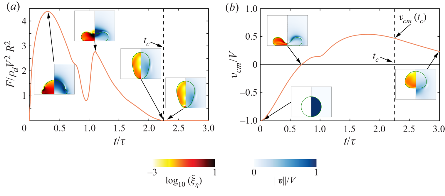
 $F$ between the substrate and the drop is zero (for calculation details, see Zhang et al. Reference Zhang, Sanjay, Shi, Zhao, Lv and Lohse2022), as shown in figure 8(a). Subsequently, we read out the centre of mass velocity (figure 8b) at this instant. If this centre of mass velocity is not in the upward direction (i.e. it is zero or negative), we categorise the case as non-bouncing. For the representative case in figure 8,
 $\varepsilon = 0.47$.
A representative temporal variation of (a) the normal reaction force  $F$ on the drop and (b) its centre of mass velocity
 $v_{cm}$. Time is normalised using the inertio-capillary time scale
 $\tau$. Insets illustrate the different stages of the drop impact process. The background shows the magnitude of the rate of viscous dissipation per unit volume (
 $\tilde {\xi }_\eta = 2Oh(\tilde {\boldsymbol {\mathcal {D}}}:\tilde {\boldsymbol {\mathcal {D}}})$) on the left and the magnitude of velocity field normalised by the impact velocity on the right. The vertical dashed black line represents the contact time calculated using the criterion
 $F = 0$, marking the end of contact between the drop and the substrate. Here,
 $(We, Oh, Bo) = (4, 0.034, 0.5)$, the contact time
 $t_c = 2.25\tau$ and the coefficient of restitution
 $\varepsilon = 0.47$.
Appendix B. Influence of Weber number
We report that the bouncing inhibition and drop contact time are fairly insensitive to an increase in the impact Weber number ( $We$) while the restitution coefficient decreases monotonically with
 $We$. Figure 9 illustrates the variation of the restitution coefficient with
 $We$ at different
 $Oh$ and fixed
 $Bo = 0.167$, enabling comparison with the experimental data of Jha et al. (Reference Jha, Chantelot, Clanet and Quéré2020). In the so-called inviscid drop limit (
 $Oh \lesssim 0.01$), the coefficient of restitution is approximately equal to the prefactors
 $\varepsilon _0(We)$ and
 $\varepsilon _*(We)$ used in § 4, (4.4) and (4.6), respectively.
Variation of the restitution coefficient with the impact Weber number ( $We$) at different drop Ohnesorge numbers (
 $Oh$). The simulations (circle data points) match perfectly with the experimental results (diamond data points) of Jha et al. (Reference Jha, Chantelot, Clanet and Quéré2020) without any fitting parameters. Here, the Bond number (
 $Bo$) is
 $0.167$.
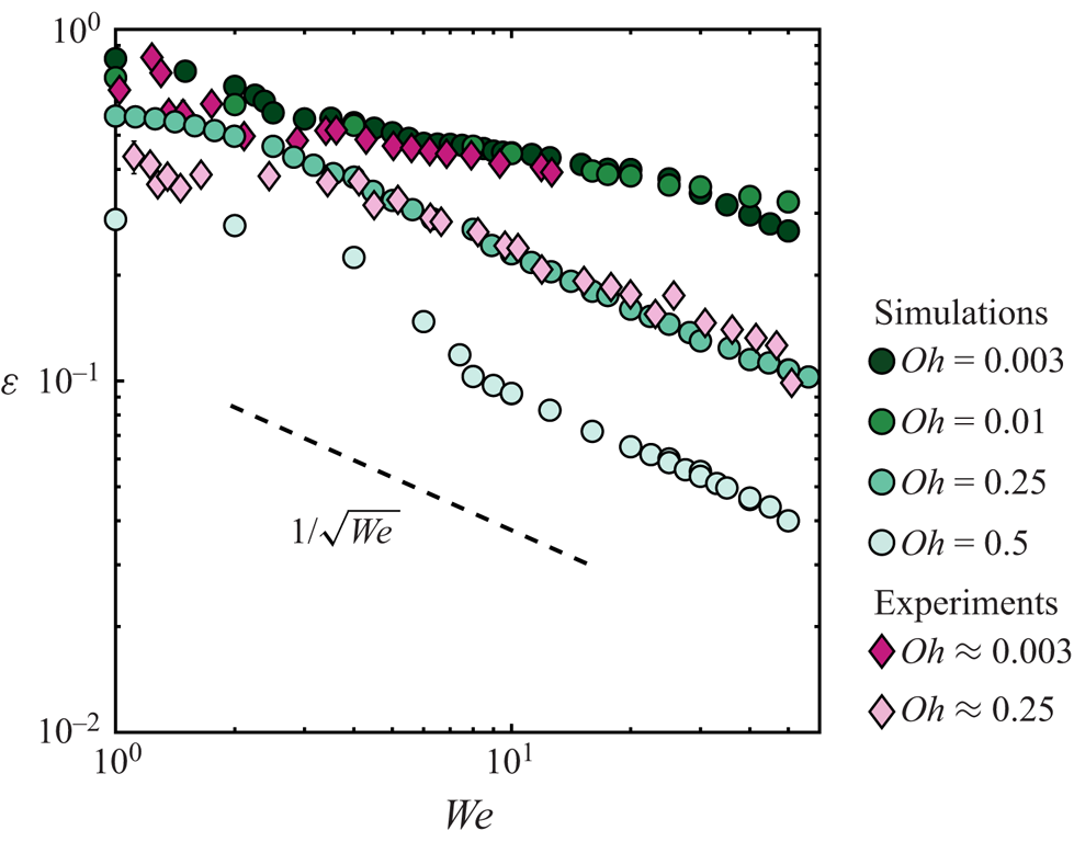
For  $Oh \lesssim 0.01$,
 $\varepsilon$ does not follow the
 $1/\sqrt {We}$ scaling relation derived by Biance et al. (Reference Biance, Chevy, Clanet, Lagubeau and Quéré2006) using a spring–mass model that neglects the influence of the drop viscosity. Indeed, the energy budgets reported in figures 5(c,d) and 7(c,d) evidence that the transfer to surface energy at take-off
 ${\rm \Delta} E_\gamma (t_c)$, proposed by Biance et al. (Reference Biance, Chevy, Clanet, Lagubeau and Quéré2006) to account for the loss of rebound elasticity, negligibly contributes to the decrease of
 $\varepsilon$ with
 $We$. Instead, we find that the increase of viscous dissipation with
 $We$ drives the decrease of
 $\varepsilon$, even in the so-called inviscid limit.
Interestingly, the restitution coefficient for viscous drop impacts ( $Oh \gtrsim 0.1$) seems to follow the
 $1/\sqrt {We}$ scaling relation, implying that the take-off velocity scales with the Taylor–Culick-type velocity (
 $v_{cm}(t_c) \sim \sqrt {\gamma /\rho _dR}$), and is independent of the impact velocity
 $V$, consistent with our assumption that the retraction and take-off stages are independent of the impact Weber number. We caution here that the range of
 $We$
 $(1 \le We \le 50)$ is too small to claim this scaling relation convincingly.
Lastly, notice the remarkable agreement between our simulations and the experimental data points from Jha et al. (Reference Jha, Chantelot, Clanet and Quéré2020) for two different drop Ohnesorge numbers, which differ by over two orders of magnitude (see figure 9).


 Open access

