1 Introduction
The fluid mechanics of flapping wings is a subject of long-standing interest to biologists. More recently, it has also attracted attention in the context of unmanned air vehicles.
Experimental work in this field has benefited greatly from the emergence of particle image velocimetry (PIV) as a viable non-intrusive full-field measurement technique. As a result, velocity data from unsteady wing-flow tests are typically available to an unprecedented extent. Force data, however, are less easily obtained. The conventional load-cell-based approach which is so successful for steady flows becomes less straightforward; the force levels in the parameter ranges relevant to flapping flight are typically much lower than for conventional wings, and measurements are contaminated by inertial loads. Hence, there is interest in alternative techniques that make use of the readily available velocity data, via the link between force and momentum.
The standard starting point (e.g. van Oudheusden et al. Reference van Oudheusden, Scarano, Roosenboom, Casimiri and Souverein2007) is a force–momentum balance for a control volume enclosing the wing. This requires knowledge of the pressure on the outer boundaries. Direct measurement of this quantity is difficult, but in incompressible flow it is fully determined by the velocity field. Hence, most momentum-based load estimates include a pressure calculation as a first step (cf., for example, Unal, Lin & Rockwell Reference Unal, Lin and Rockwell1997; van Oudheusden, Casimiri & Scarano Reference van Oudheusden, Casimiri and Scarano2008; Mohebbian & Rival Reference Mohebbian and Rival2012; Gharali & Johnson Reference Gharali and Johnson2014). Alternatively, the dependence of pressure on velocity allows the primitive control-volume formulation to be manipulated into one that is pressure-free, at the price of greater complexity in the boundary flux terms (Noca, Shiels & Jeon Reference Noca, Shiels and Jeon1999; Simão Ferreira et al. Reference Simão Ferreira, van Bussel, van Kuik and Scarano2011; DeVoria & Ringuette Reference DeVoria and Ringuette2013). At present, it is unclear whether this step conveys a significant practical advantage. Common to both methods is the possibility of accuracy problems when organised flow structures cross the boundary (Mohebbian & Rival Reference Mohebbian and Rival2012; DeVoria & Ringuette Reference DeVoria and Ringuette2013).
An alternative to the control-volume approach is one based on the impulse of the flow field. Historically, the deduction of force from impulse is linked to first potential, and then inviscid, flow theory, but it has since been shown (Wu Reference Wu1981) that the formulae arising in these contexts are special cases of a general result for a real viscous fluid. The impulse-based formulation is attractive because it eliminates the need to calculate pressure (or equivalent) contributions at a boundary. It also has the potential to provide useful physical insight, as it is founded on the vorticity field. However, it requires every significant part of that field to have been captured. In particular, the details of the ‘starting’ vorticity must be available. As a result, this approach cannot be regarded as a candidate to supplant the momentum formulation in all cases. Nonetheless, where applicable, it represents a complementary, and potentially valuable, line of attack.
Examples of impulse-based load estimation are given by Lin & Rockwell (Reference Lin and Rockwell1996), Poelma, Dickson & Dickinson (Reference Poelma, Dickson and Dickinson2006) and DeVoria & Ringuette (Reference DeVoria and Ringuette2013). In each case, the starting flow is included in the available data, and the results show promising agreement with direct measurements. None, however, addresses the issue of resolution near the body surface. This is a particular concern for impulse-based methods, based as they are on the vorticity field. Vorticity generated at the surface diffuses very slowly into the bulk fluid, over periods of the order of the Reynolds number greater than the convective time scale, so the local field consists of intense spatially concentrated regions. Inevitably, not all will be properly captured by the experimental measurements, introducing an unquantifiable, and possibly significant, potential for error. The purpose of this paper is to present a means of accounting for the deficit.
The key idea is to represent the ‘missing’ vorticity as a vortex sheet on the body surface. The concept of a surface vortex sheet arises naturally for inviscid flow, as an interpretation of the physically unrealistic slip velocity that the theory permits (Lighthill Reference Lighthill and Rosenhead1963). Perhaps surprisingly, it is also useful for viscous fluids. Here, although the singular distribution of vorticity that it represents cannot occur in a physically realisable flow, it appears when the vorticity evolution equation is discretised in time. After a finite time step, the evolved vorticity field is no longer consistent with the no-slip condition on bounding surfaces. The vortex sheet associated with the discrepancy is identified as the accumulation of vorticity generated at the surface over the time step. In the real flow, such vorticity is continuously diffused into the fluid and the field remains finite; in the numerical method, the diffusion requires a separate subsequent calculation. This qualitative algorithm description was first given by Lighthill (Reference Lighthill and Rosenhead1963), and forms the basis of the ‘vortex-method’ approach to flow computation. Its implementation in practice is discussed by Cottet & Koumoutsakos (Reference Cottet and Koumoutsakos2000, chap. 6).
The approach presented in this paper bears a strong superficial resemblance to the vortex-method algorithm: the velocities associated with the (incomplete) experimental-vorticity field are inconsistent with the no-slip condition on the body surface, and the discrepancy corresponds to our vortex sheet. Conceptually, however, it is crucially different, in that the sheet cannot be directly linked to vorticity generation. Indeed, if the experimental-vorticity field were complete and fully resolved, there would be no sheet, but there would of course still be vorticity generation at the surface. Our vortex sheet is simply an approximate representation of the part of the (real finite) vorticity field that has not been captured by the experimental measurements. We argue that this must be accounted for if the impulse formulation is to be valid.
Fortunately, this is entirely possible; given the experimental-vorticity field and the body motion, the sheet strength is uniquely determined (Lighthill Reference Lighthill1986, chap. 6). (A supplementary condition may also be required. Typically, this issue only arises in two-dimensional flows, and is resolved by application of Kelvin’s circulation theorem.) In general, it would be calculated using a two- or three-dimensional panel method, but here we consider an application – two-dimensional flow around a flat plate – that is amenable to a quasi-analytical approach. The theoretical details are set out in § 2. An initial experimental assessment of the method is then presented in § 3.
2 Application: translating plate in two dimensions
2.1 Description
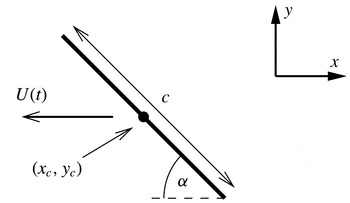
The problem geometry is defined in figure 1. A flat plate of chord
 $c$
moves parallel to the
 $x$
axis in fluid that is stationary at infinity. The plate is oriented at an angle
 $\unicode[STIX]{x1D6FC}$
to the horizontal, with centre at
 $(x_{c},y_{c})$
and speed
 $U(t)(=-\text{d}x_{c}/\text{d}t)$
. It starts from rest, with the fluid quiescent, so according to Kelvin’s theorem the circulation around a contour enclosing the plate and its shed vorticity is zero throughout the motion.
The translating flat-plate wing. The plate has chord
 $c$
and centre coordinates
 $(x_{c},y_{c})$
. It moves horizontally to the left at incidence
 $\unicode[STIX]{x1D6FC}$
and with speed
 $U(t)$
.

2.2 Vortex-sheet strength
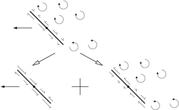
The strength of the vortex sheet is given by the spurious plate-surface slip velocity associated with the experimental-vorticity field. Thus, although it is conceptually different from the sheet that arises in a vortex method, its calculation is algorithmically identical. As noted by Eldredge (Reference Eldredge2010), it depends linearly on the plate motion and the vorticity field, so its strength can be expressed as the sum of their individual contributions. This decomposition is shown schematically in figure 2.
Schematic representation of the decomposition of the surface vortex sheet into components associated with the plate motion (left) and the experimental-vorticity field (right).

Each vortex-sheet component requires its overall circulation to be specified before it is uniquely determined. It should be noted, first, that the plate-motion part has an irrotational surrounding flow field. Therefore, if its circulation is chosen to be zero, it is simply the potential flow associated with the classical ‘added-mass’ force contribution (Batchelor Reference Batchelor2000, § 6.4). While it is not intuitively obvious that added mass should persist in this form even when the overall flow is strongly rotational, Leonard & Roshko (Reference Leonard and Roshko2001, appendix) have convincingly argued that it must. Hence, we follow Eldredge (Reference Eldredge2010), and make this term non-circulatory. The other vortex-sheet component, due to the known vorticity, then has circulation equal and opposite to that of the known vorticity. It will henceforth be referred to as the ‘circulatory part’ of the vortex sheet.
The expression for the vortex-sheet strength is most conveniently found by conformal mapping. In terms of the complex variable
 $$\begin{eqnarray}z=(x-x_{c})+\text{i}(y-y_{c}),\end{eqnarray}$$
the mapping defined by
 $$\begin{eqnarray}z=\unicode[STIX]{x1D701}+\left(\frac{c}{4}\text{e}^{-\text{i}\unicode[STIX]{x1D6FC}}\right)^{2}\unicode[STIX]{x1D701}^{-1}\end{eqnarray}$$
transforms the plate into the cylinder
 $\unicode[STIX]{x1D701}=(c/4)\text{e}^{\text{i}\unicode[STIX]{x1D703}}$
, with
 $\unicode[STIX]{x1D703}$
denoting angular position. The problem is now to determine the flow around the cylinder, subject to the plate motion and the known vorticity. The former appears straightforwardly as an oncoming free stream with horizontal velocity
 $U$
, but the latter requires further consideration. Without loss of generality, we represent the vorticity field as a collection of point vortices with circulations
 $\unicode[STIX]{x1D6E4}_{k}$
at locations
 $(x_{k},y_{k})$
. The mapping of (2.2) conserves circulation, so the
 $\unicode[STIX]{x1D701}$
plane contains point vortices
 $\unicode[STIX]{x1D6E4}_{k}$
at the positions
 $$\begin{eqnarray}\unicode[STIX]{x1D701}_{k}=\frac{1}{2}\left[z_{k}+\left(z_{k}-\frac{c}{2}\text{e}^{-\text{i}\unicode[STIX]{x1D6FC}}\right)^{1/2}\left(z_{k}+\frac{c}{2}\text{e}^{-\text{i}\unicode[STIX]{x1D6FC}}\right)^{1/2}\right],\end{eqnarray}$$
with
 $z_{k}$
defined in terms of
 $x_{k}$
and
 $y_{k}$
by (2.1).
According to the circle theorem (Batchelor Reference Batchelor2000, § 6.5), the cylinder-surface boundary condition can be satisfied by introducing, for each vortex, images of circulation
 $-\unicode[STIX]{x1D6E4}_{k}$
and
 $\unicode[STIX]{x1D6E4}_{k}$
at
 $\unicode[STIX]{x1D701}=(c/4)^{2}/\unicode[STIX]{x1D701}_{k}^{\ast }$
and
 $\unicode[STIX]{x1D701}=0$
respectively. However, this leaves the cylinder with zero circulation, rather than the required value
 $-\sum \unicode[STIX]{x1D6E4}_{k}$
, which must therefore be added via an additional point vortex at the origin. Since this element exactly cancels all of the image vortices at that point, we conclude that the known-vorticity contribution to the cylinder flow can equally be found by simply introducing the
 $-\unicode[STIX]{x1D6E4}_{k}$
images alone.
The upshot of these considerations is a complete description of the cylinder-plane flow, consisting of contributions from the known point vortices, their images and the oncoming free stream. The quantity of interest is the azimuthal velocity,
 $u_{\unicode[STIX]{x1D703}}$
, on the cylinder surface, and this can be written as
 $$\begin{eqnarray}u_{\unicode[STIX]{x1D703}}=u_{\unicode[STIX]{x1D703}}^{c}+u_{\unicode[STIX]{x1D703}}^{am},\end{eqnarray}$$
with
 $$\begin{eqnarray}\displaystyle & \displaystyle u_{\unicode[STIX]{x1D703}}^{c}=-\frac{2}{\unicode[STIX]{x03C0}c}\mathop{\sum }_{k}\unicode[STIX]{x1D6E4}_{k}\frac{|\unicode[STIX]{x1D701}_{k}|^{2}-(c/4)^{2}}{|\unicode[STIX]{x1D701}_{k}-(c/4)\text{e}^{\text{i}\unicode[STIX]{x1D703}}|^{2}}, & \displaystyle\end{eqnarray}$$
 $$\begin{eqnarray}\displaystyle & \displaystyle u_{\unicode[STIX]{x1D703}}^{am}=-2U\sin \unicode[STIX]{x1D703}. & \displaystyle\end{eqnarray}$$
It should be noted that this split mirrors the plate-plane decomposition of figure 2;
 $u_{\unicode[STIX]{x1D703}}^{c}$
is the circulatory part associated with the known-vorticity field and
 $u_{\unicode[STIX]{x1D703}}^{am}$
is the added-mass term. Their link to the plate-plane vortex-sheet strength will be explained in the following section.
2.3 Impulse
The impulse components are given by the area integrals (Wu Reference Wu1981),
 $$\begin{eqnarray}I_{x}=\int y\unicode[STIX]{x1D714}\,\text{d}A,\quad I_{y}=-\int x\unicode[STIX]{x1D714}\,\text{d}A,\end{eqnarray}$$
where
 $\unicode[STIX]{x1D714}$
is the vorticity field. (Wu extends this quantity to the interior of the moving body as well, but the additional contribution to the impulse is zero in our case.) It should be recalled that, here,
 $\unicode[STIX]{x1D714}$
consists of both the known vorticity in the fluid and the surface vortex sheet required to fulfil the no-slip boundary condition. The former is represented by the point vortices
 $\unicode[STIX]{x1D6E4}_{k}$
and the latter will be denoted as
 $\unicode[STIX]{x1D6FE}$
. Hence, (2.7) becomes
 $$\begin{eqnarray}I_{x}=I_{x}^{kv}+I_{x}^{vs},\quad I_{y}=I_{y}^{kv}+I_{y}^{vs},\end{eqnarray}$$
with
 $$\begin{eqnarray}I_{x}^{kv}=\mathop{\sum }_{k}y_{k}\unicode[STIX]{x1D6E4}_{k},\quad I_{y}^{kv}=-\mathop{\sum }_{k}x_{k}\unicode[STIX]{x1D6E4}_{k}\end{eqnarray}$$
and
 $$\begin{eqnarray}I_{x}^{vs}=\oint y\unicode[STIX]{x1D6FE}\,\text{d}l,\quad \mathop{I}_{y}^{vs}=-\oint x\unicode[STIX]{x1D6FE}\,\text{d}l,\end{eqnarray}$$
the contour integrals being taken around the plate surface.
To evaluate the vortex-sheet contributions, we must link
 $\unicode[STIX]{x1D6FE}$
to the mapped cylinder flow field. To do so, we first view the latter in the same way, i.e. as a combination of surrounding vorticity and a vortex sheet on the body surface. The vortex-sheet strength is then given by the tangential slip velocity,
 $u_{\unicode[STIX]{x1D703}}$
(cf. (2.5) and (2.6)). Furthermore, the circulation-conserving property of the plate–cylinder mapping implies the relation
 $$\begin{eqnarray}\unicode[STIX]{x1D6FE}\,\text{d}l=u_{\unicode[STIX]{x1D703}}\frac{c}{4}\,\text{d}\unicode[STIX]{x1D703},\end{eqnarray}$$
which allows the integrals of (2.10) to be found without derivation of an explicit expression for
 $\unicode[STIX]{x1D6FE}$
. Finally, then, in terms of the separate components of
 $u_{\unicode[STIX]{x1D703}}$
,
 $$\begin{eqnarray}I_{x}^{vs}=I_{x}^{c}+I_{x}^{am},\quad I_{y}^{vs}=I_{y}^{c}+I_{y}^{am},\end{eqnarray}$$
where
 $$\begin{eqnarray}I_{x}^{c}=\frac{c}{4}\int _{0}^{2\unicode[STIX]{x03C0}}y|_{\unicode[STIX]{x1D701}=(c/4)\text{e}^{\text{i}\unicode[STIX]{x1D703}}}u_{\unicode[STIX]{x1D703}}^{c}\,\text{d}\unicode[STIX]{x1D703},\quad I_{y}^{c}=-\frac{c}{4}\int _{0}^{2\unicode[STIX]{x03C0}}x|_{\unicode[STIX]{x1D701}=(c/4)\text{e}^{\text{i}\unicode[STIX]{x1D703}}}u_{\unicode[STIX]{x1D703}}^{c}\,\text{d}\unicode[STIX]{x1D703},\end{eqnarray}$$
 $$\begin{eqnarray}I_{x}^{am}=\frac{c}{4}\int _{0}^{2\unicode[STIX]{x03C0}}y|_{\unicode[STIX]{x1D701}=(c/4)\text{e}^{\text{i}\unicode[STIX]{x1D703}}}u_{\unicode[STIX]{x1D703}}^{am}\,\text{d}\unicode[STIX]{x1D703},\quad I_{y}^{am}=-\frac{c}{4}\int _{0}^{2\unicode[STIX]{x03C0}}x|_{\unicode[STIX]{x1D701}=(c/4)\text{e}^{\text{i}\unicode[STIX]{x1D703}}}u_{\unicode[STIX]{x1D703}}^{am}\,\text{d}\unicode[STIX]{x1D703}.\end{eqnarray}$$
The plate-plane
 $x$
and
 $y$
coordinates in these expressions are defined by (2.2) and (2.1). It should be noted that this formulation, despite its representation in the cylinder plane, evaluates the contributions to the plate-plane impulse in the absolute frame of reference (i.e. with the fluid stationary at infinity). We also observe in passing that, in this particular application, the integrals of (2.13) can be evaluated in closed form, via residue theory (Wang & Eldredge Reference Wang and Eldredge2013).
Finally, as shown by Wu (Reference Wu1981), the (two-dimensional) drag and lift forces on a body of negligible cross-sectional area (the general result includes an additional, straightforwardly calculable, term associated with the inertia of the fluid displaced by the body) are given by
 $$\begin{eqnarray}D_{2D}=-\unicode[STIX]{x1D70C}\frac{\text{d}I_{x}}{\text{d}t},\quad L_{2D}=-\unicode[STIX]{x1D70C}\frac{\text{d}I_{y}}{\text{d}t}.\end{eqnarray}$$
These expressions also define the forces associated with the various impulse components, via (2.8) and (2.12).
At this stage, it is worth recalling that Wu’s results apply for a viscous fluid; i.e. the forces found via (2.15) include both pressure and shear-stress contributions. This point deserves emphasis because of the aforementioned similarity between the current approach and the enforcement of the no-slip boundary condition in a vortex method. We reiterate that the vortex sheet here is not purely associated with vorticity generation, and is hence not directly linked to the surface pressures. Instead, it represents the unmeasured part of the vorticity field, which, when complete, determines the overall fluid force through the impulse relation.
3 Experimental assessment
This section presents an initial evaluation of the proposed method, using PIV velocity-field data and force-balance measurements. As two-dimensional flow is difficult to achieve experimentally, the test case is three-dimensional, and the impulse analysis is based on a single plane in the velocity field. Support for this approach comes from the investigations of Luttges (Reference Luttges1989), Jones, Pitt Ford & Babinsky (Reference Jones, Pitt Ford and Babinsky2011) and Jardin, Farcy & David (Reference Jardin, Farcy and David2012), which have found starting flows to be quasi-two-dimensional. Nonetheless, it introduces a discrepancy between the theoretical assumptions and the experiment which must be borne in mind.
3.1 Apparatus and measurements
The experimental facility has already been documented by Pitt Ford & Babinsky (Reference Pitt Ford and Babinsky2013), so it will only be described briefly here. It consists of a 7 m-long by 1 m-square towing tank, through which a rectangular carbon-fibre flat-plate wing is transported by a carriage. For the tests reported here, the plate has chord 0.12 m and span 0.48 m. A skim plate on the carriage end provides a symmetry plane, so the effective aspect ratio is 8. Force measurements are made with a two-component strain-gauge balance and velocity measurements using PIV. The wing position is found from its image in the PIV frames.
3.2 Test cases
For all tests reported here, the incidence was set to a nominal angle of
 $45^{\circ }$
and the wing was translated over 10 chords with a constant-acceleration/constant-velocity/constant-deceleration profile. Two different profiles were investigated, with acceleration to final velocity over one-chord or six-chord displacement. For both, the deceleration to rest was over the final chord of motion.
In order to optimise data quality, force and PIV measurements were carried out at different Reynolds numbers, 35 000 and 10 000 (based on final velocity and chord). The justification for this approach rests on previous observations (Tangler & Ostowari Reference Tangler and Ostowari1991; Ol et al. Reference Ol, Altman, Eldredge, Garmann and Lian2010) of Reynolds-number independence for high-incidence aerofoil flows with well-defined separation points.
In all cases, the PIV measurement plane was at half-span.
3.3 Data processing
3.3.1 Position tracking
The wing appears as a thin white line in the raw PIV images. Its position was determined using a template-matching algorithm, starting from manually determined estimates for vertical coordinate and angle. In a first pass through the images, matching was performed for horizontal coordinate and angle simultaneously, displacement normal to chord and displacement tangent to chord. The resulting vertical-coordinate estimates showed a slight increasing trend inconsistent with the nominal trajectory, and confirmed as spurious by direct inspection of velocity fields. A second pass was thus made with vertical position fixed at an (approximate) average value, with the matching over horizontal coordinate and angle repeated. Both first- and second-pass angle estimates also showed a trend, from approximately
 $46.6^{\circ }$
to
 $47.4^{\circ }$
. For subsequent analysis, the wing angle was taken as
 $47^{\circ }$
. The uncertainty in final results associated with the angle and vertical-coordinate discrepancies is discussed in § 3.5.
The impulse calculation requires a value for the instantaneous wing velocity that is robust to the subsequent differentiation required to deduce force. This was obtained by least-squares fitting of the estimated position to its nominal form. For the six-chord acceleration-distance case, the acceleration is constant throughout the PIV field of view, and the fit was unconstrained. In contrast, the one-chord case reaches its final velocity within the field of view, and the fit was constrained to have one-chord displacement at this point. Both fits showed excellent agreement with the tracked position data, with root-mean-square errors in the region of 0.2 mm. The kinematic parameters obtained from the fits are given in table 1.
Trajectory parameters for the PIV runs.

For the force-measurement runs, in the absence of tracking information, a trigger channel providing start and stop markers was employed. The kinematic parameters deduced from the overall times and nominal position profiles of the runs are shown in table 2.
Trajectory parameters for the force-measurement runs.

3.3.2 Velocity-field analysis
Each velocity field was estimated from the average of five experimental runs. Details of the PIV analysis are given by Pitt Ford & Babinsky (Reference Pitt Ford and Babinsky2013).
The quantities required here are the elemental circulations
 $\unicode[STIX]{x1D6E4}_{k}$
, which define the known-vorticity contribution to impulse explicitly, via (2.9), and the circulatory vortex-sheet contribution implicitly, via the term
 $u_{\unicode[STIX]{x1D703}}^{c}$
in (2.13). They were found by direct trapezoidal integration around each (square) data-grid cell. The associated position coordinates were set to the cell-centre values.
All of the velocity fields are incomplete. Most notably, the region directly below the wing is shaded from the laser light sheet and contains no reliable data. Elsewhere, a number of grid points have velocity vectors identified as spurious during the PIV data processing. These non-physical contributions must be excluded from the impulse calculation. Equally, it is advantageous for numerical efficiency to ignore regions of irrotational flow.
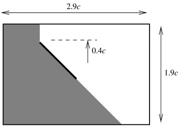
The upshot of these considerations is indicated schematically in figure 3, which shows the wing at a representative position in the PIV field of view. The shaded area both contains the unreliable light-sheet shadow region and is expected, on physical grounds, to be irrotational (with the exception of an attached boundary layer on the plate underside, which will be accounted for by the vortex sheet). Hence, the cell-circulation analysis was restricted to the remaining white part of the field. Within this area, only contributions from cells with legitimate velocity vectors at all four corners (the vast majority) were considered.
The flat-plate wing in the PIV field of view, showing overall dimensions and the approximate vertical position of the plate. Data in the shaded region are excluded from the calculation of the experimental-vorticity impulse contribution.

3.3.3 Force-balance data
Each case was repeated five times, and the results were averaged to obtain normal and tangential force records. High-frequency noise was removed by filtering and downsampling (from 2 kHz to 200 Hz), using a proprietary decimation routine (http://uk.mathworks.com/help/signal/ref/decimate.html). No further smoothing was applied. The forces were then resolved into the
 $x$
and
 $y$
directions, using the incidence deduced from the tracking analysis.
Rig-inertia effects were characterised by running the same displacement profiles in the emptied tow-tank. The effective inertia was found by least-squares fitting to the point-mass force profile associated with the nominal acceleration history. This quantity was used to calculate, and subtract, the rig-inertia force in the filled-tank runs.
3.4 Results
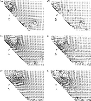
The finite PIV field of view (cf. figure 3), along with the need to capture all of the shed vorticity, limits the available impulse data to the first two chords of plate travel. Sample plate-region velocity fields from this part of the motion are presented in figure 4.
Particle image velocimetry velocity fields in the vicinity of the plate. Panels (a,c,e) are for acceleration over one chord, with plate displacements of (a)
 $c/2$
(
 $t=1.4c/U_{0}$
), (c)
 $c$
(
 $t=2c/U_{0}$
) and (e)
 $3c/2$
(
 $t=2.5c/U_{0}$
). Panels (b,d,f) show the six-chord acceleration results for the same displacements, with times (b)
 $3.5c/U_{0}$
, (d)
 $4.9c/U_{0}$
and (f)
 $6c/U_{0}$
. The arrows marked ‘
 $U$
’ and ‘
 $U_{0}$
’ indicate the instantaneous and final plate velocities respectively. Also plotted are contours of dimensionless vorticity,
 $\unicode[STIX]{x1D714}c/U$
, at levels
 $-30$
,
 $-20$
,
 $-10$
, 10, 20 and 30.

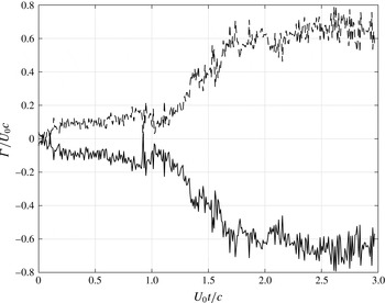
Figure 5 shows the evolution of the measured circulation with time in the one-chord acceleration case. The notable feature of this plot is the departure of the circulation from the zero value that would be found if all of the vorticity were captured by the experimental data. By the end of the record, the discrepancy is approximately
 $0.7U_{0}c$
, which is significant. (A wing in steady flow with bound circulation at this level would have a lift coefficient of 1.4.) Figure 5 also includes the circulation associated with the plate vortex sheet, calculated in the same way as the corresponding impulse components. This provides a useful algorithmic check – as required, it is equal and opposite to the measured value – and a means of assessing the required discretisation. Two hundred panels were used, yielding a typical accuracy of better than 0.01 %.
Experimental (——) and vortex-sheet (– – –) circulations for the one-chord acceleration case.

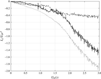
An example of the calculated impulse – the
 $x$
component in the one-chord acceleration case – is shown in figure 6. Also plotted are its two constituents according to the decomposition of (2.8): the known-vorticity (2.9) and vortex-sheet (2.10) contributions. Both are seen to be relevant. The reduced ‘noise’ in the overall curve should also be noted; we ascribe this to the compensating effect of the vortex-sheet calculation. There will inevitably be some variation in the extent of near-plate vorticity captured by the PIV measurements, but any circulation lost here must, due to the Kelvin-theorem constraint, reappear in the vortex sheet. Furthermore, as long as the missed vorticity is not too far from the plate, its substitute in the sheet will be located appropriately, and will thus give the correct contribution to the impulse.
Horizontal impulse for the one-chord acceleration case: ——, experimental-vorticity contribution; – – –, vortex-sheet contribution;
 $\cdots \cdots$
, total.

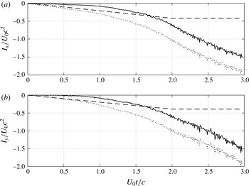
The decomposition of the impulse into known-vorticity and vortex-sheet contributions is dependent on the resolution of the measurements near the plate. Hence, it is of algorithmic, rather than physical, interest. Figure 7 shows, for both components of the impulse, an alternative: into circulatory
 $(I_{x}^{kv}+I_{x}^{c},I_{y}^{kv}+I_{y}^{c})$
and added-mass
 $(I_{x}^{am},I_{y}^{am})$
contributions. The latter increase linearly with time during the (one-chord) acceleration phase up to
 $t=2U_{0}/c$
, and remain constant thereafter. This, of course, is exactly the behaviour expected of the added mass. It is also possible to confirm correspondence between the current formulation and the classical added-mass concept; the forces deduced from the gradients match the theoretical results for the flat plate (which can be derived analytically from the general expressions given by, for example, Batchelor Reference Batchelor2000, § 6.4).
Horizontal (a) and vertical (b) impulse components for the one-chord acceleration case: ——, vortical contribution; – – –, added-mass contribution;
 $\cdots \cdots$
, total.

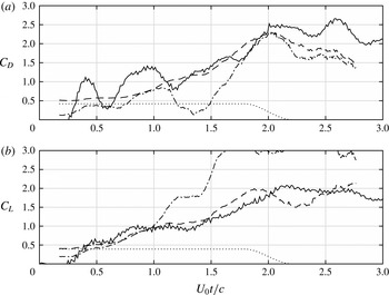
The drag- and lift-coefficient predictions obtained from the impulses of figure 7, via (2.15), are compared with the direct force measurements in figure 8. The numerical differentiation was performed via a linear least-squares fit over a window of 0.5 s centred on the time of interest. (The filtering effect of this method can be seen in the added-mass contribution.) The non-dimensionalisation is on
 $(\unicode[STIX]{x1D70C}U_{0}^{2}c)/2$
. For the force-balance data, the corresponding quantity is
 $2\unicode[STIX]{x1D70C}U_{0}^{2}c^{2}$
(recall that the wing span is
 $4c$
). Also shown are the predictions that would arise if the impulse were calculated from the experimental-vorticity field alone, without the vortex-sheet contribution.
Drag (a) and lift (b) coefficients for the one-chord acceleration case: ——, force-balance data; – – –, impulse-based prediction; — ⋅ —, prediction from experimental-vorticity impulse alone;
 $\cdots \cdots$
, added-mass contribution to the prediction.

It is immediately evident that this component is crucial. Without it, the predictions bear little relation to the direct measurements. When it is included, the agreement is much better, albeit still imperfect at a detailed level. (It should be noted, however, that the large-scale measured-force oscillations are probably associated with vibration, and hence spurious.) Finally, the benefit of being able to identify the added-mass contribution is clear; we see that this term initially dominates, but is gradually superseded by the circulatory part.
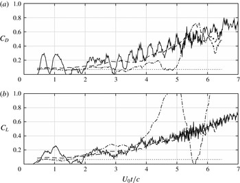
All results presented so far have been for the one-chord acceleration case, which includes the transition from constant acceleration to constant velocity within the PIV field of view. We conclude with the force comparison for the six-chord acceleration case (figure 9). Here, an impulse-differentiation fitting window of 1.0 s was employed. The direct measurement is significantly noisier than previously, but it is still possible to discern good agreement – if anything, better than in figure 8 – with the impulse-based prediction, as long as the vortex-sheet contribution is accounted for. Added mass again represents a dominant proportion of initial force levels but (unlike the one-chord case) becomes almost insignificant before the acceleration phase is complete.
Drag (a) and lift (b) coefficients for the six-chord acceleration case: ——, force-balance data; – – –, impulse-based prediction; — ⋅ —, prediction from experimental-vorticity impulse alone;
 $\cdots \cdots$
, added-mass contribution to the prediction.

3.5 Errors and uncertainty
3.5.1 Direct force measurements
The precision error of the force balance is 0.01 N (Pitt Ford & Babinsky Reference Pitt Ford and Babinsky2013), which corresponds to an absolute uncertainty of
 $3\times 10^{-3}$
in the force coefficients of figures 8 and 9. These results are also affected by the choice of incidence angle, which was set to
 $47^{\circ }$
on the basis of the tracking analysis. The uncertainty associated with the range observed there (
 $46.6^{\circ }$
–
 $47.4^{\circ }$
) can be estimated on the basis that the overall force on the plate is predominantly in the normal direction. This implies a relative uncertainty of 0.7 %.
In practice, the variance of the force-measurement ensembles for each case implies considerably greater uncertainty than the estimates above. This quantity is reasonably constant as a function of time, allowing the standard deviation of the ensemble means to be estimated at approximately 0.1 N, corresponding to an absolute uncertainty in drag and lift coefficients of 0.03.
3.5.2 Forces derived from impulse
The most obvious error path for this calculation is from the PIV velocity data, for which the error estimates are given by Pitt Ford & Babinsky (Reference Pitt Ford and Babinsky2013). Unfortunately, the propagation is not straightforward to predict; while the summations of (2.9) imply a beneficial reduction in variation, there is also significant cancellation in the cell-circulation calculation. Certainly, as shown in figure 6, there are notable fluctuations in the impulse estimates. However, these occur on a time scale much shorter than the fitting window used for differentiation, which was deliberately chosen to include a large number of time samples (50 in this case). Hence, in the expected absence of significant correlation in time, we argue that stochastic uncertainty in the velocity data is likely to be unimportant. This leaves the bias error of
 $-1\,\%$
(Pitt Ford & Babinsky Reference Pitt Ford and Babinsky2013), which would feed through directly.
A more subtle, but more important, issue is the influence of estimated plate position on the force predictions. This was assessed by running the analysis again for alternative parameter specifications. For the plate incidence, values of
 $46.6^{\circ }$
and
 $47.4^{\circ }$
were specified, and found to yield variations typically under 1 %, with extremes exceeding 2 % only very rarely. Similar differences were found for vertical positions 2 mm either side of the nominal value.
3.6 Discussion
While inevitably limited, the results of this initial assessment clearly support our fundamental contention: that an impulse-based force prediction method must account for vorticity near the body surface that is either unavailable or unresolved in the experimental data. Without its contribution, the impulse yields force estimates of little, if any, utility. Its inclusion improves the quality of prediction to a level that, if not perfect, is usable. Furthermore, these conclusions are not compromised by uncertainties in the data analysis.
Strictly, the demonstration applies only to the current measurements. However, as argued before, it is hard to envisage any present-day experimental data set that fully resolves the vorticity field at practical Reynolds numbers, so some degree of augmentation will always be necessary. The quantitative significance of such augmentation will, of course, vary, and this is a topic for further investigation. Similarly, the relative accuracy of impulse-based and control-volume approaches remains an open question.
A secondary conclusion follows from the correspondence between the impulse-based method (as implemented here) and the direct measurements: strong two-dimensionality in the unsteady flow, at least during the starting phase. While important on its own, this observation also has significance for the approach proposed here. If the flow is two-dimensional, not only are data requirements reduced, but the vortex-sheet calculation is simplified, and the impulse-based approach becomes particularly attractive. Equally, starting flows form an ideal context for its application (because of the need for complete vorticity-field information). Thus, if the tendency towards two-dimensionality observed here is indeed a general feature of starting flows, the proposed method will be a natural choice for force estimation.
Finally, it is worth mentioning that the idea of using the experimental velocity field and the body boundary condition to correct for data incompleteness could also be used in momentum-based force calculations. Under the same conditions as assumed here – all missing vorticity close to the body – the combined experiment/vortex-sheet system uniquely determines the velocity field at all points in the fluid. Hence, unavailable or spurious velocities in irrotational regions of a control volume could be reconstructed.
4 Conclusions
In this paper, we have proposed an impulse-based method for estimating body forces, given velocity-field data. Its novelty lies in allowance for incompleteness in the data, via a surface vortex sheet introduced to ensure that the no-slip boundary condition is satisfied. We argue that experimental measurements from high-Reynolds-number flows are inevitably incomplete to some extent; even the best quality and most extensive sets will fail to resolve high-shear regions close to the body. However, these are exactly the locations where the vortex sheet compensates correctly for missing data. Thus, as long as there are no significant lacunae away from the body, the upshot is a complete flow description which will provide accurate impulse estimates.
To illustrate the method, we have set out the necessary analysis for the case of a translating plate in two dimensions. We have then applied the resulting formulation to experimental data for which direct force measurements are also available. The significance of the surface vortex sheet in this instance has been demonstrated, with its contributions both materially altering the overall impulse levels and compensating, to some extent, the noise in the measured-vorticity component. Finally, the force predictions arising from the impulse calculation have been shown to agree satisfactorily with the direct measurements. Implicit in this agreement is a high degree of two-dimensionality in the (three-dimensional) experiment.
The prospects for the proposed method thus appear good. In particular, it is well suited to starting flows, where the requirement for measurements to span the entire vorticity field is most easily met. The case is even more compelling if, as is the case here, the flows are essentially two-dimensional; data need only be collected on a plane, and the vortex-sheet calculation is simplified.
We conclude by reiterating the theoretical attraction of an impulse-based method: it allows flow features to be linked with body forces, thereby providing insight and understanding. However, these benefits are crucially dependent on the availability of a complete, physically consistent, description of the vorticity field. We argue that, at the Reynolds numbers of interest, this is highly unlikely to be provided purely by experimental data; hence, we recommend the introduction of a surface vortex sheet to enforce the no-slip condition in all impulse-based force calculations.
Acknowledgements
The second author thanks the Engineering and Physical Sciences Research Council (EPSRC) for financial support via its ‘Doctoral Training’ scheme. The paper itself has benefited significantly from the thorough appraisal provided by its reviewers. Supporting research data are available at: https://www.repository.cam.ac.uk/handle/ 1810/261928.