




No CrossRef data available.
Article contents
Nematode parasites of sheep: extension of a simple model to include host variability
Published online by Cambridge University Press: 18 November 2004
Abstract
We use results from a simulation-based model of nematode infection of sheep to refine the parameters in a simpler generic model of host–parasite population dynamics. These parameters describe the following host–parasite traits: probability of establishment of ingested larvae, mortality rate of adult parasites, and fecundity of adult female parasites. This simple model is then extended by allowing those parameters to vary amongst individual hosts. A sensitivity analysis is performed to determine which parameters have most influence on host parasite burden. The establishment parameter has the greatest effect on the peak value of parasite burden whilst the other two parameters have more effect on the duration of the burden. A comparison is made with results from the flock model after discussion of the definition of an average host. By allowing these parameters to vary simultaneously within the individual hosts we are able to reproduce the over-dispersed distribution of adult parasites frequently seen in nematode infections of sheep flocks.
Information
- Type
- Research Article
- Information
- Copyright
- 2005 Cambridge University Press
INTRODUCTION
For nematode infections of domestic sheep, the modelling literature has fallen into two distinct types: simulation-based models e.g. Barnes & Dobson (1990a,b), Leathwick, Barlow & Vlassoff (1992) and mechanistic, dynamic models e.g. Grenfell (1988), Roberts & Heesterbeek (1995), Kao et al. (2000).
The simulation-based models are usually very detailed and are constructed in close association with experimental studies (Paton, Thomas & Waller, 1984; Smith & Galligan, 1988; Smith & Grenfell, 1994). Their main purpose has been to evaluate control measures in specific regions or circumstances, as for example in Australia (Barnes & Dobson 1990a,b). By contrast, the simpler dynamic models (Roberts & Grenfell, 1991; Roberts & Heesterbeek, 1995) have been used to elucidate general principles applicable to all control situations. All these models have thus far focussed on the flock and their outcomes are usually average values (Callinan et al. 1982; Roberts & Grenfell, 1991, 1992; Smith et al. 1999).
Management practices that control for mean levels of parasitism may risk unacceptably high levels of parasitism in individual animals, where the recourse to treatment is a last resort, or unnecessary treatment of lambs with low or nil infections, in a conventional system where intervention is based on a mean count. The level of infection within a flock is not normally distributed, but skewed, with the majority of individuals with nil or a low level and a few with high levels (Barger, 1985). The individual animal's ability to avoid or withstand larval infection relies on a variety of factors: genotype, grazing behaviour, current diet, nutrient reserves and physiological state and stress. Understanding more about how each of these factors influences the performance of individual animals under a parasite challenge offers scope for developing strategies for preventing unnecessary suffering or treatment. There will also be interactions that occur between a number of these factors and the difficulty of controlling these individually under experimental conditions necessitates a modelling approach.
Generally speaking, healthy adult sheep (>12 months age) and ewes outside lactation or parturition have negligible parasite burdens. They typically maintain a high level of immunity to parasites and are almost fully resistant to worm establishment unless put under stress. In this paper we therefore concentrate on young lambs (up to 12 months) which, with minimal anthelmintic intervention, would generally harbour the majority of the adult parasites and would be responsible for most of the contamination with eggs that give rise to larvae on the pasture.
THE MODEL
We briefly review the variables and parameters in the previously published simple generic model on which our extended individual model is based (Roberts & Grenfell, 1991, 1992). Most of the detailed processes described explicitly in the simulation-based models are subsumed into a few rate mechanisms and are expressed as differential equations (DEs) for the appropriate state variables. The three state variables of the model are the mean number of adult nematodes per host A, the pasture density (per m2 or ha) of infective nematode larvae L, and the mean level of immunity in the host r (modelled as cumulative larval challenge). The model variables are defined in Table 1 and the dynamics are described by the following DEs:


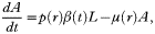

- Infective nematode larval density: This DE expresses the fact that infective larvae are lost from pasture by either host ingestion or other factors such as mortality, and regained by the successful development of new larvae from worm eggs deposited on the pasture in host faeces.
- Adult nematodes per host: This DE states that the mean worm burden (number of adult parasites) per host increases by ingestion of infective larvae which successfully develop into adult worms, and decreases due to worm mortality. The probability of successful development of ingested larvae to adult stage and worm mortality both depend on the host immunity level.
- Level of immunity: This DE models host immunity as cumulative larval intake and allows immunity to decline in the absence of larval intake. As pointed out by Kao et al. (2000), the use of cumulative larval intake as a proxy for host immune response is potentially controversial. Nevertheless, it does capture, in the simplest manner, the observation that prolonged exposure to larvae is necessary for the development and maintenance of the host immune response.
In the analysis of this model to date, the time dependence of β and ρ has been ignored, along with the host immunity dependence of the adult parasites' fecundity and mortality rates (Kao et al. 2000). This is because previous work has focussed on the effect(s) of management decisions on between-, rather than within-year dynamics. A good example of this would be resetting adult parasite numbers and host immunity at the beginning of each year to describe newborn lambs being introduced on to previously contaminated pasture. When using the model to examine within-year dynamics, varying pasture consumption rate during the year and the effect of host immunity on adult parasite fecundity and mortality become more important. We have obtained better estimates for these by incorporating some of the input and results from a simulation model for nematodiasis in New Zealand lambs (Leathwick et al. 1992). Specifically, the pasture consumption rate β now depends on host age and is assumed to be zero in the first 2 weeks, thereafter increasing in a sigmoid fashion to a plateau value of 1·45 kg DM d−1 for a mature host. The mortality rate of parasites increases with time, and since immunity level (cumulative larval intake) also increases with time, we can determine the relationship between mortality rate and immunity level.
The extended individual host model
The flock model above has output variables of mean parasite burden, mean immunity level and pasture larval density. We now consider a group of n individual hosts, each of which might possess different pasture consumption rates, larval establishment probabilities, and parasite mortality and fecundity rates. The basis for this difference between individuals is probably genetic and we would expect some correlation between the latter three traits. For example, a host with a lower probability of larval establishment than another with the same level of immunity would also be expected to have higher parasite mortality and lower parasite fecundity rates. It has been conjectured that much of the observed variation in parasite burden between hosts is attributable to host heterogeneity (Grenfell et al. 1995; Cornell, Isham & Grenfell, 2004). The following model will enable us to explore the consequences of allowing some of the most important host characteristics to vary individually. The corresponding DEs to (1) become:



where the subscript i runs from 1 to n for the n hosts. We use l to indicate number of infective larvae and

to stand for the larval intake rate by the ith host at time t. This is a slightly different interpretation for β(t) than used before so we have indicated this by inserting a tilde, (β(t) has units of m2 week−1 whereas
will have units of week−1). Each host carries its own adult parasite burden Ai and immune status ri.
The establishment rate probability pi(ri), adult parasite mortality μi(ri) and fecundity λi(ri) depend on the individual host's immune status and may also vary for each host, even when those hosts have the same immune status. One simplifying assumption would be to amend this so that individual hosts are distinguished only by differences in their immune status. In that case we are dealing with a group of genetically identical hosts (clones). However, differences in immune status could still arise through varying larval ingestion rates or immunity fade rates. In dealing with clones we can drop the first subscript i in the adult parasite parameters pi(ri), μi(ri) and λi(ri) so that each individual will have the same adult parasite establishment probability, mortality and fecundity as other hosts with the same immunity status.
Parameter values
Here we present the functional forms used for the parameters appearing in Table 2.

The probability that an ingested larva develops into an adult parasite decreases as host immunity increases, and for the ith host (i=1 to n) we assume this is given by

A graph of this function for various values of ki is shown in Fig. 1A. The value of p0 (probability of an ingested larva developing into an adult parasite in an immunologically naïve host with r=0) can vary from 0·35 to 0·77 depending on parasite species (Kao et al. 2000).
The parameter ki controls how rapidly the probability of an ingested larvae developing successfully to an adult parasite in host i declines with that host's increasing immune status.

Fig. 1. The variation amongst individuals of the 3 host–parasite traits considered in the model. The most resistant host is represented by the solid curves and the least resistant host by the dashed-dotted curves. Two other hosts with intermediate resistance are also shown (dotted and dashed curves).
The mortality rate of adult parasites increases as host immunity increases, and for the ith host (i=1 to n) we assume this is given by

A graph of this function for various values of mi is shown in Fig. 1B. The value of μ0 is the common mortality rate when all hosts have reached full immunity. The parameter mi controls the point of inflection occurring in the function defined by equation (4). Kao et al. (2000) use constant values for the mortality rate ranging from 0·01 d−1 to 0·11 d−1 depending on parasite species.
The fecundity rate of adult parasites decreases as host immunity increases, and for the ith host (i=1 to n) we assume this is given by

A graph of this function for various values of fi is shown in Fig. 1C. The value of λ0 is the common fecundity rate for immunological naïve hosts with r=0. The parameter fi controls the point of inflection occurring in the function defined by equation (5). Kao et al. (2000) used constant values for the fecundity rate ranging from 150 eggs d−1 to 6300 eggs d−1 (per adult female) depending on parasite species.
For the purposes of the present model the pasture consumption rate is assumed not to vary between hosts but will increase with age. Consumption of pasture is zero for host age less than 2 weeks and thereafter is given by the relationship of Leathwick et al. (1992)
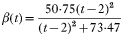
where t is the age of the host in weeks and the units of β are m2 week−1. To convert this parameter for use in the individual model we need to divide β by the grazing area a as noted previously. We have assumed the pasture cover is uniform at 0·2 kg DM m−2 throughout the year so consumption of 1·45 kg DM d−1 is equivalent to grazing 50·75 m2 week−1.
Because the host immunity level r is being modelled by cumulative larval intake, its value ranges from zero (immunologically naïve) to millions (full immunity). Thus the values for parameters ki, mi and fi appearing in (3)–(5) above will be of the order 10−6, 106 and 106 respectively to ensure a reasonable range of response as the immunity level increases from zero to its final value. For the purpose of demonstrating the effect of individual host variability we choose (i) ki to vary uniformly from 23×10−6 (most resistant) to 5×10⁻⁶ (least resistant), (ii) mi to vary uniformly from 0·1×106 (most resistant) to 4·6×106 (least resistant) and (iii) fi to vary uniformly from 0·1×106 (most resistant) to 1·9×106 (least resistant).
By most resistant we mean that at a given level of immunity this host has the lowest probability of ingested larvae developing to adult parasite, and the highest mortality and lowest fecundity rates for its adult parasites. For large groups of hosts the variation in these parameters is more likely to be normally distributed (Niezen, Waghorn & Charleston, 1998; Harrison et al. 1999; Leathwick et al. 1999; Hong, Michel & Lancaster, 1986; Sutherland et al. 1997). We chose a uniform distribution with small host numbers for illustrative purposes. The other parameter values used are given in Table 2 and are constant in producing the results in Figs 2 and 3 and during the sensitivity analysis of the next section.
Sensitivity analysis
Because there is considerable variation in the values for ki, mi and fi and uncertainty in their field measurement, a sensitivity analysis was undertaken. Sensitivity analyses assist in identifying those parameters responsible for greatest perturbations in the model output and whose values must be known most precisely. To do this in a systematic fashion, one parameter set was varied at a time using the base values prescribed for ki, mi and fi in the preceding section. Ten hosts were modelled varying each set of ki, mi and fi by ±50%. For example, to test the sensitivity of the model to variation in establishment of ingested larvae, we allowed ki to vary uniformly from 34·5×10−6 to 7·5×10−6 (+50%) and then from 11·5×10−6 to 2·5×10−6 (−50%) with mi and fi as prescribed before. The results are shown in Figs 2A through 2C. In these figures and the remainder of this section, the 10 hosts start with zero worm burdens and graze a 1 ha field which initially has 106 infective larvae on it. For clarity of presentation we have shown worm burdens for only the most and least resistant hosts.

Fig. 2. Results from the parameter sensitivity analysis for host–parasite traits in a group of 10 hosts. Graphs A to C (column 1), D to F (column 2) and G to I (column 3) are from varying the parameters controlling establishment probability, mortality rate and fecundity rate respectively. The solid curves show results when default parameter values for the 10 hosts were used. The dotted and dashed curves resulted from varying the default parameter set by minus and plus 50% respectively.
The effect of varying ki on pasture larval density, worm burdens for the most and least resistant host, and the host immunity are shown in Fig. 2A and C respectively. There are considerable differences in the peak values of larval density and worm burdens. Also note that the worm burden in the least resistant host is sustained for much longer; the adult parasites in this host being largely responsible for the secondary peak in larval density seen after day 200, when climatic conditions are again conducive to larval establishment from their deposited eggs. The primary peak in larval density lags the peak in worm burden for the most resistant host, but of course every host is contributing to the larvae on pasture, so the timing of these peaks is not sequential as in the identical host case. Because we are assuming the larval intake and immunity fade rates for each host are the same, in Fig. 2C the immunity status for each host will remain identical if they start with the same value.
We now reset ki to the default values and vary the mortality rate parameter mi. The results are shown in Fig. 2D–F. The most striking difference here is that the peak values of pasture larval density and worm burdens show almost no change as mi varies (Fig. 2D and E). However, both the pasture larval densities and worm burdens for the least resistant host remain at different levels through to 365 days, whereas for varying ki the values came together by that time. The host immunities in Fig. 2F also remain very similar for considerably longer here (about 150 days). This would go some way to explaining why the peak worm burdens remain at approximately the same level in Fig. 2E.
Finally we examine the sensitivity of the results to varying the fecundity parameter fi. These results are displayed in Fig. 2G–I. There are larger dif-ferences in the value of the second peak of pasture larval density (Fig. 2G), which is not entirely unexpected as this would be the output most directly affected by changes in fecundity. There is no difference in the value or timing for the peak of the worm burdens (Fig. 2H) and the difference in worm burden, though again sustained through to day 365, is not as great as when varying mi. The changes in host immunity are intermediate compared to the two previous cases (Fig. 2I): a divergence is apparent about day 120 which then grows as before through to day 365.
In terms of worm burden, clearly the most sensitive parameter is ki associated with establishment of ingested larvae as adult parasites. To some extent this reflects the functional form we have chosen to represent this process. However, when the establishment probability is plotted as a function of time and compared with the corresponding graph from running the simulation model of Leathwick et al. (1992), there is very little difference in the result. This indicates that the functional form we have chosen can be justified on the basis of field data.
The three parameters considered in this section are unlikely to vary independently within a group of hosts. For example, we would expect individuals with a high value of ki to have both lower values for mi and fi. Thus, when comparing two groups, increasing ki for each individual within that group should also be accompanied by decreasing values for both mi and fi for every individual. This would tend to reinforce the trends already seen in Fig. 2.
Comparison with flock model
To demonstrate clearly the connection between the individual and flock models, we consider first the simplest case of n indistinguishable hosts grazing on an area a. That is, we have n genetically identical individuals which are also grazing in an identical manner. The DE in equation (2c) shows that the immune status of every host will remain identical if they started with the same immune status. Thus we can drop the subscript i from the variables A and r in equations (2b) and (2c), and equation (2a) becomes

On dividing this DE through by the grazing area a we get

where H is the host density n/a and L is the pasture larval density l/a. Thus the DEs are identical with the flock model in equations (1a–c) as long as we take

(which also makes their units agree).
We next examine the case where individuals are identical except for one varying host parasite trait and compare with the flock model. This differs from the sensitivity analysis of the preceding section in that only one host parasite trait is allowed to vary whilst the other two traits are held constant (at the flock value) between hosts. For the sensitivity analysis each host had three different parameter values describing the three parasite traits.
There are two obvious ways in which we can define an average value for the varying host parasite trait so that comparison can be made with the flock model. The first is to use the median value of the parasite parameter. With μ(r) and λ(r) held fixed at the flock values, consider a group of ten individual hosts with ki varying uniformly from 23×10−6 (most resistant) to 5×10⁻⁶ (least resistant). The median value of ki for this group of ten hosts is

, and we define the median establishment probability as

Alternatively, we could use the mean establishment probability, defined as
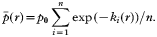
This differs considerably from the median probability, particularly at higher levels of immunity. Note that these definitions do not actually depend on the parameter ki being uniformly distributed. The critical assumption is that the form of p(r) is identical for each individual and that host heterogeneity can be described by variation in ki.
It is straightforward to show from the governing DEs of the individual model that if we use this mean establishment probability as the group average, and define the mean worm burden as

, then the outcomes from the individual and flock models will be identical (see Appendix). This result is not true if we use the median establishment probability

as the group average.
Now hold p(r) and μ(r) fixed at the flock values and vary the fecundity parameter fi only. Equation (2b) shows that in this case every host has the same worm burden over time if all hosts started with the same burden. Using this result in equation (2a) renders it identical to equation (1a) as long as we define the group average fecundity as

. Again, this result is not true were we to use the median fecundity as the group average.
Lastly, hold p(r) and λ(r) fixed at the flock values and vary the mortality parameter mi only. Equation (2b) shows that worm burden will now be different for each host. Furthermore, there is now no definition of a group average mortality for adult worms that will make this DE agree with its flock counterpart in (1b).
As already noted when we first introduced the individual model, the parameters describing the host parasite traits are unlikely to vary independently, and are more likely to be related with one another. Thus, when comparing hosts, one that has a lower probability for establishment of ingested larvae is also likely to have a higher adult parasite mortality and lower adult parasite fecundity. When the parameters are varied at the same time in this manner, (i.e. high ki implies both low mi and low fi for the ith individual) there is a large degree of over-dispersion in the distribution of the adult worm burden. In other words, a plot of flock fraction against worm burden would not be a Poisson distribution but would be significantly skewed, with most of the flock having low or moderate burdens whilst a small fraction of the flock possesses very high burden. This is because the above host–parasite traits interact strongly to produce far greater burdens than if the traits were not related. To demonstrate this, the contribution to the total worm burden in a flock of 10 individuals by the 2 least resistant hosts is shown in Fig. 3. For comparative purposes, also plotted in the figure is the same contribution by the two least resistant hosts when the host–parasite traits are varied singly (i.e. are assumed to be not related). As before, we assume the flock is grazing on a 1 ha field which initially contains 106 larvae and use the default host parasite parameters from the sensitivity analysis section. When each of the parasite parameters is varied, the other two parameters are set at the mean flock value as defined above. From Fig. 3 we see also that host variation in mortality rate of adult parasites has the greatest effect on the proportion of the parasite population present in susceptible individuals. However, it is only when the parasite parameters are all allowed to vary that the fraction of total worm burden carried by the two least resistant hosts of the flock reaches a value nearing 80%. This provides further confidence in the parameter values used as these figures are supported by field measurements where parasite populations are generally found to be over-dispersed with the majority of hosts generally carrying few worms and a few are heavily infected and harbour the majority of the total parasite population (Barger, 1985; Sréter et al. 1994).

Fig. 3. Demonstration of the over-dispersed worm burden distribution that occurs when the host–parasite traits vary simultaneously for 10 hosts (solid curve). Also shown for comparative purposes are the distributions when these traits vary singly. The dotted, dashed and dashed-dotted curves show the results from varying only the mortality rate, establishment probability and fecundity rate respectively.
DISCUSSION
The extended individual host model developed in this paper has many similarities with the original flock model (Roberts & Grenfell, 1991, 1992) and has identical outcomes when mean values are used for all the parasite parameters. When a parasite parameter varies with each individual host (the other two parameters remaining at their mean values) the outcome will depend on which parameter is varying. If it is ki, associated with establishment of ingested larvae, then each host will have a different parasite burden. The mean burden will be identical to the outcome given by the flock model when using the mean establishment parameter defined previously. Varying only fi that controls adult female parasite fecundity, results in each host having an identical parasite burden. The pasture larval density will also be identical to the outcome given by the flock model using the mean fecundity parameter. However, when varying the mortality parameter mi, neither the parasite burden nor pasture larval density will agree with the outcome from the flock model, no matter how we define the mean mortality. To sum up, the individual and flock model outcomes will agree if the parameters ki and fi are varied amongst the hosts, but will not agree when the parameter mi is varied. This occurs because ki is associated with increase in worm burden due to larval ingestion from pasture and all individual hosts contribute to this larval load. Thus an increase in mean worm burden can be calculated from a corresponding mean larval ingestion. When mortality of adult parasites varies amongst hosts the mean worm burden can no longer be calculated in this simple manner.
Our individual model may be used in a number of different ways. It is still simple enough for deriving control thresholds and understanding the long-term (between-year) dynamics of nematode populations. In this regard it shares the advantages of the flock model on which it is based. However, there is also sufficient flexibility inherent in the parasite parameters to examine individual variability in response to short-term control measures e.g. drenching/selective drenching of a proportion of a flock and the overall effect of breeding programmes designed to produce more resistant hosts (Bisset et al. 2001). There is an increasing interest in alternative methods for controlling nematodes in sheep such as these breeding programmes, better grazing management and timely use of different stock classes because of the escalating incidence of nematodes resistant to currently available anthelmintics in New Zealand (Leathwick, Pomroy & Heath, 2001). The outcomes of this kind of modelling exercise could have considerable practical implications in the management of parasitism by providing general trends that may be expected when varying the parameters describing the host–parasite traits.
In focussing on the probability of larval establishment, adult parasite mortality and fecundity, together with the manner in which these traits depend on host immunity, we have greatly simplified a complex parasitological scenario. Moreover, as our model's description of host immunity is basically equivalent to cumulative larval intake, this assumption needs to be examined more critically and refined in future models. However, dependence on host immunity notwithstanding, the advantage of being able to manipulate these parameters is that alternative control methods might be evaluated more precisely. As seen from the sensitivity analysis, any method which can reduce the proportion of ingested larvae establishing as adult parasites will have a far greater impact on parasite burden than a method which kills, or reduces the fecundity of those parasites, once established. This is especially important for the less resistant hosts. In contrast, the sensitivity analysis reveals that variation in the traits has little impact on larval numbers on pasture, with all traits having almost equivalent effect. This argument must be considered more carefully when considering the impact on long-term (between-year) dynamics. The results from Fig. 2 show that pasture larval density at the end of the year are at very similar levels to their starting values, irrespective of which host–parasite trait is varied. There are a few extended studies of larvae on pasture in several areas of New Zealand, with ewes and lambs, and lambs after weaning, in most instances under low or no control scenarios (as in the model). Under these conditions in the field larval numbers returned to a similar level at the end of each winter. In one longitudinal study of the larval population on pasture over 3 years (Vlassoff, 1976), numbers returned to <500 larvae/kg green grass in August/September which is about the same as the model's assumption of 106 larvae ha−1 and 0·2 kg DM m−2.
It might be of interest to use this model to compare and contrast the long-term effects of different control measures. For example, anthelmintic treatment removes the majority of the worm burden from every host and this will obviously have large impact on eggs produced and larvae developed for ingestion by the hosts grazing in the following years. However, because in this model larval intake is necessary for development of immune response, such treatment might not be as effective in the long run as a vaccine which instead reduces the fecundity of any worms present. Thus, in the latter case, enough eggs and hence larvae are still being produced to stimulate the host immune response but not at a level to cause very high worm burdens and production losses.
Our model's focus on individual variability also allows for more precisely targeted control measures, whether conventional or novel. We have demonstrated that even for a small flock of animals this individual variability leads to a small proportion of hosts carrying the majority of the total flock parasite burden. This aggregation has been observed in many host–parasite systems but detailed data sets for nematodes in sheep are rare (Barger, 1985; Hong, Michel & Lancaster, 1987). In the flock model, of course, the total worm burden must by definition be evenly distributed amongst the hosts. If the most susceptible hosts could be identified early in life and treated, or even removed from the flock, it is likely that much lower pasture larval contamination will occur later, resulting in benefits for the remaining animals. Indeed, this is the rationale behind the breeding programme for more resistant hosts already mentioned (Bisset et al. 2001).
Future development of the model will incorporate the effect of parasitism on host live weight. Again, the focus will be on the individual host; in particular examining why growing lambs show such large variation in weight gain when grazing as flocks on contaminated pasture. Because weight gain is one of the key measures of productivity, the ability to maintain the gain under parasitic challenge is extremely important. An extended model such as the one proposed is necessary if alternative control methods, such as biocontrol agents for reducing infective larvae numbers on pasture, breeding programme selecting animals for resilience to parasites, management practices including the strategic use of ‘clean’ forages, etc are to be rigorously evaluated. This approach provides an insight into the relative value of each option and under what circumstances each is most effective, assists in identifying our knowledge gaps and helps determine whether further experimental work is warranted.
This work was carried out as part of New Zealand Foundation for Research, Science and Technology Contract C10X0236. We would like to thank Dr Andy Bray and Mr Deane Carson of AgResearch (Lincoln); Dr Annette Litherland and Mr Keith Betteridge of AgResearch (Grasslands); Dr Simon Lovatt and Mr Chris Boom of AgResearch (Ruakura) for their input during the development phase of the model.
APPENDIX
We are considering the individual model where only the establishment probability pi(r) varies between the hosts. The mortality and fecundity rates for each host are identical and equal to the flock values. In this case equations (2a–c) become
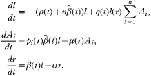
We sum the second of these DEs over all hosts i and divide by the total number of hosts n to obtain

which simplifies to
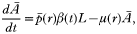
where Ā is the mean worm burden and

is the mean establishment probability as defined in equation (6). Thus, using this definition of an average value
for the hosts, the DEs reduce to those of the flock model in (1a–c). This is not the case if we use the alternative median establishment probability

. Similar analysis can be carried out when only the mortality or fecundity vary between hosts with the other two parasite traits held constant.
References
REFERENCES
BARGER, I. A. (
1985).
The statistical distribution of Trichostrongylid nematodes in grazing lambs.
International Journal for Parasitology 15,
645–649.CrossRefGoogle Scholar
BARNES, E. H. &
DOBSON, R. J. (
1990 a).
Population dynamics of Trichostrongylus colubriformis in sheep: mathematical model of worm fecundity.
International Journal for Parasitology 20,
375–380.Google Scholar
BARNES, E. H. &
DOBSON, R. J. (
1990 b).
Population dynamics of Trichostrongylus colubriformis in sheep: computer model to simulate grazing systems and the evolution of anthelmintic resistance.
International Journal for Parasitology 20,
823–831.Google Scholar
BISSET, S. A.,
MORRIS, C. A.,
McEWAN, J. C. &
VLASSOFF, A. (
2001).
Breeding sheep in New Zealand that are less reliant on anthelmintics to maintain health and productivity.
New Zealand Veterinary Journal 49,
236–246.CrossRefGoogle Scholar
CALLINAN, A. P. L.,
MORLEY, F. H. W.,
ARUNDEL, J. H. &
WHITE, D. H. (
1982).
A model of the life cycle of sheep nematodes and the epidemiology of nematodiasis in sheep.
Agricultural Systems 9,
199–225.CrossRefGoogle Scholar
CORNELL, S. J.,
ISHAM, V. S. &
GRENFELL, B. T. (
2004).
Stochastic and spatial dynamics of nematode parasites in farmed ruminants.
Proceedings of the Royal Society of London, Series B 271,
1243–1250.CrossRefGoogle Scholar
GRENFELL, B. T. (
1988).
Gastrointestinal nematode parasites and the stability and productivity of intensive ruminant grazing systems.
Philosophical Transactions of the Royal Society of London, B 229,
47–67.CrossRefGoogle Scholar
GRENFELL, B. T.,
WILSON, K.,
ISHAM, V. S.,
BOYD, H. E. G. &
DIETZ, K. (
1995).
Modelling patterns of parasite aggregation in natural populations: trichostrongylid nematode–ruminant interactions as a case study.
Parasitology 111,
S135–S151.CrossRefGoogle Scholar
HARRISON, G. B. L.,
PULFORD, H. D.,
GATEHOUSE, T. K.,
SHAW, R. J.,
PFEFFER, A. &
SHOEMAKER, C. B. (
1999).
Studies on the role of mucus and mucosal hypersensitivity reactions during rejection of Trichostrongylus colubriformis from the intestine of immune sheep using an experimental challenge model.
International Journal for Parasitology 29,
459–468.CrossRefGoogle Scholar
HONG, H. A.,
MICHEL, J. F. &
LANCASTER, M. B. (
1986).
Populations of Ostertagia circumcincta in lambs following a single infection.
International Journal for Parasitology 16,
63–67.CrossRefGoogle Scholar
HONG, H. A.,
MICHEL, J. F. &
LANCASTER, M. B. (
1987).
Observations on the dynamics of worm burdens in lambs infected daily with Ostertagia circumcincta.
International Journal for Parasitology 17,
951–957.CrossRefGoogle Scholar
KAO, R. R.,
LEATHWICK, D. M.,
ROBERTS, M. G. &
SUTHERLAND, I. G. (
2000).
Nematode parasites of sheep: a survey of epidemiological parameters and their application in a simple model.
Parasitology 121,
85–103.CrossRefGoogle Scholar
LEATHWICK, D. M.,
BARLOW, N. D. &
VLASSOFF, A. (
1992).
A model for nematodiasis in New Zealand lambs.
International Journal for Parasitology 22,
789–799.CrossRefGoogle Scholar
LEATHWICK, D. M.,
VLASSOFF, A. &
BARLOW, N. D. (
1995).
A model for nematodiasis in New Zealand lambs: the effect of drenching regime and grazing management on the development of anthelmintic resistance.
International Journal for Parasitology 25,
1479–1490.CrossRefGoogle Scholar
LEATHWICK, D. M.,
MILLER, C. M.,
BROWN, A. E. &
SUTHERLAND, I. A. (
1999).
The death rate of Ostertagia circumcincta and Trichostrongylus colubriformis in lactating ewes: implications for anthelmintic resistance.
International Journal for Parasitology 27,
411–416.Google Scholar
LEATHWICK, D. M.,
POMROY, W. E. &
HEATH, A. C. G. (
2001).
Anthelmintic resistance in New Zealand.
New Zealand Veterinary Journal 49,
227–235.CrossRefGoogle Scholar
NIEZEN, J. H.,
WAGHORN, G. C. &
CHARLESTON, W. A. G. (
1998).
Establishment and fecundity of Ostertagia circumcincta and Trichostrongylus colubriformis in lambs fed lotus (Lotus pedunculatus) or perennial ryegrass (Lolium perenne).
Veterinary Parasitology 78,
13–21.CrossRefGoogle Scholar
PATON, G.,
THOMAS, R. J. &
WALLER, P. J. (
1984).
A prediction model for parasitic gastro-enteritis in lambs.
International Journal for Parasitology 14,
439–445.CrossRefGoogle Scholar
ROBERTS, M. G. &
GRENFELL, B. T. (
1991).
The population dynamics of nematode infections of ruminants: periodic perturbations as a model for management.
IMA Journal of Mathematics Applied in Medicine and Biology 8,
83–93.CrossRefGoogle Scholar
ROBERTS, M. G. &
GRENFELL, B. T. (
1992).
The population dynamics of nematode infections of ruminants: the effect of seasonality in the free-living stages.
IMA Journal of Mathematics Applied in Medicine and Biology 9,
29–41.CrossRefGoogle Scholar
ROBERTS, M. G. &
HEESTERBEEK, J. A. (
1995).
The dynamics of nematode infections of farmed ruminants.
Parasitology 110,
493–502.CrossRefGoogle Scholar
SMITH, G. &
GALLIGAN, D. T. (
1988).
Mathematical models of the population biology of Ostertagia ostertagi and Teladorsagia circumcincta, and the economic evaluation of disease control strategies.
Veterinary Parasitology 27,
73–83.CrossRefGoogle Scholar
SMITH, G. &
GRENFELL, B. T. (
1994).
Modelling of parasite populations: gastrointestinal nematode models.
Veterinary Parasitology 54,
127–143.CrossRefGoogle Scholar
SMITH, G.,
GRENFELL, B. T.,
ISHAM, V. &
CORNELL, S. (
1999).
Anthelmintic resistance revisited: underdosing chemoprophylactic strategies and mating probabilities.
International Journal for Parasitology 29,
77–91.CrossRefGoogle Scholar
SRÉTER, T.,
MOLNÁR, V. &
KASSAI, T. (
1994).
The distribution of nematode egg counts and larval counts in grazing sheep and their implications for parasite control.
International Journal for Parasitology 24,
103–108.CrossRefGoogle Scholar
SUTHERLAND, I. A.,
LEATHWICK, D. M.,
BROWN, A. E. &
MILLER, C. M. (
1997).
Prophylactic efficacy of persistent anthelmintics against challenge with drug-resistant and susceptible Ostertagia circumcincta.
The Veterinary Record 141,
120–123.CrossRefGoogle Scholar
VLASSOFF, A. (
1976).
Seasonal incidence of infective trichostrongyle larvae on pasture: the contribution of the ewe and the role of the residual pasture infestation as sources of infection to the lamb.
New Zealand Journal of Experimental Agriculture 4,
281–284.CrossRefGoogle Scholar
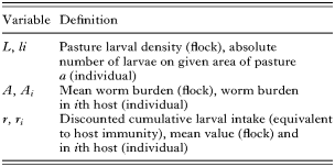
Table 1. Definition of model variables
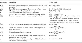
Table 2. Definition of model parameters
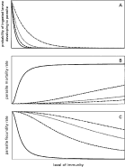
Fig. 1. The variation amongst individuals of the 3 host–parasite traits considered in the model. The most resistant host is represented by the solid curves and the least resistant host by the dashed-dotted curves. Two other hosts with intermediate resistance are also shown (dotted and dashed curves).
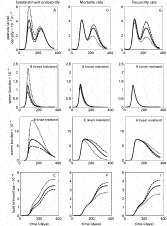
Fig. 2. Results from the parameter sensitivity analysis for host–parasite traits in a group of 10 hosts. Graphs A to C (column 1), D to F (column 2) and G to I (column 3) are from varying the parameters controlling establishment probability, mortality rate and fecundity rate respectively. The solid curves show results when default parameter values for the 10 hosts were used. The dotted and dashed curves resulted from varying the default parameter set by minus and plus 50% respectively.
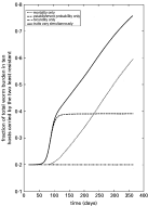
Fig. 3. Demonstration of the over-dispersed worm burden distribution that occurs when the host–parasite traits vary simultaneously for 10 hosts (solid curve). Also shown for comparative purposes are the distributions when these traits vary singly. The dotted, dashed and dashed-dotted curves show the results from varying only the mortality rate, establishment probability and fecundity rate respectively.
 You have
Access
- 18
- Cited by