Notation

• x Distance along the flume (cm)

• z Vertical distance from the bottom (cm)

• g Gravity acceleration (m s⁻²)

• l ₀ Length of the initial saline solution (cm)

• h ₀ Initial height of the saline solution (cm)

• H Initial water height (cm)

• ϕ = h ₀/H

• u Velocity in the x direction (m s⁻¹)

• x _f Distance covered by the front of the gravity current (cm)

• u _f Front velocity (cm s⁻¹)

• ρ _a Ambient fluid density (Mg m^s−3)

• ρ ₀ Saline solution initial density (Mg m⁻³)

• ρ Density of the gravity current (Mg m⁻³)

• t Time (s)

• Fr Froude number

• x _s = l ₀(3 + 7.4 h ₀/H) Slump distance (cm)

• y = x − x _s (cm)

• r Ambient fluid entrainment ratio

• A ₀ (l ₀ h ₀) Initial volume per unit width

Introduction

A gravity current is the flow of a heavy fluid into a light one. It is produced by the gravitational force applied to the difference in density between both fluids. The density contrast can be due to differences in temperature, composition or bulk properties of suspensions. Some examples of such currents are: submarine turbidity, pyroclastic flows released during volcanic eruptions, powder-snow avalanches, etc. The study of these phenomena in situ is very difficult. In order to determine the laws governing the dynamics of these flows, physical models have been elaborated and developed in laboratories. The use of scale models allows flexibility in experimentation and the possibility of controlling the slope, the released volume, the initial composition and the position of obstacles. Several papers have been published on this topic by Reference Hopfinger and Tochon-Danguy.Hopfinger and Tochon-Danguy (1977), Reference Huppert and SimpsonHuppert and Simpson (1980), Reference SimpsonSimpson (1987), Reference Beghin and OlagneBeghin and Olagne (1991), Reference Hermann and HutterHermann and Hutter (1991) and Reference Hallworth, Phillips, Huppert and Sparks.Hallworth and others (1993, Reference Hallworth, Phillips, Huppert and Sparks.1996). Numerical models have also been developed in order to understand and predict the behaviour of powder avalanches. Three-dimensional numerical models have been proposed by Reference Brandstatter, Hagen, Sampl and SchaffhauserBrandstatter and others (1992), Reference Bonnecaze, Hallworth, Huppen and ListerBonnecaze and others (1993), Reference Hermann, Issler, Keller, Buisson and BrugnotHermann and others (1993) and Reference NaaimNaaim (1995). To validate such models, numerical results are compared to experimental ones obtained from scale models. Earlier studies have provided many data on front velocity, the geometry of currents (height and length), particle concentration and entrainment of the ambient fluid. The aim of the present study is to complete these data, in the ease of a two-dimensional gravity current on a horizontal bottom, by internal measurements of the density and velocity. By using image-processing techniques and a salt-concentration measurement device, we obtained the concentration and velocity profiles inside the gravity current during its flow. It has been shown by Reference Brandstatter, Hagen, Sampl and SchaffhauserBrandstatter and others (1992), Reference Hermann, Issler, Keller, Buisson and BrugnotHermann and others (1993) and Reference NaaimNaaim (1995) that the proposed numerical model reproduces well global observations such as the height and the front velocity. The new experimental results will be used to lest our numerical model reproducing the internal density and velocity evolution.

Horizontal Bottom Gravity Current

Many studies have been undertaken to define the dynamics of gravity currents. In 1940, von Kármán showed theoretically that a gravity current of density ρ and height h (height of the head), in a less dense fluid of infinite depth, propagates with a front velocity:

(1)

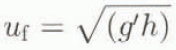
where g′ is the reduced gravity.

These studies have provided a large amount of data concerning the front velocity in relation to the distance covered. Reference BenjaminBenjamin (1968) improved the initial formula of von Kármán by including a coefficient dependent on the height of the gravity current in the expression for the front velocity. u _f becomes:

(2)

The different phases in the flow of a gravity current on a horizontal bottom are characterized by different dynamics of propagation. A more detailed Observation reveals noticeable variations in the front velocity along the flow. Reference Huppert and SimpsonHuppert and Simpson (1980) have elaborated a theoretical model of propagation. They observed that the ratio of front height to water height (h/H = ϕ) plays an important role in flow velocity. The influence of ϕ on the flow has been discussed theoretically by Reference BenjaminBenjamin (1968) and the proposed evolution of the Froude number has been verified by Reference Britter and SimpsonBritter and Simpson (1978)

(3)

(4)

The expression of the front velocity found in this way depends on the density, front height and the ratio ϕ. The analysis proposed by Reference Huppert and SimpsonHuppert and Simpson (1980) is based on two-dimensional spreading of a finite volume of a dense fluid. Initially, the height of the dense fluid is equal to the height of the water (H). A vertical water gate separates the two fluids. The authors have shown experimentally that the flow goes through two successive stages before the effects of the viscosity become dominant. The transition between the two stages takes place when the wave generated by the reflection of the counter-current upstream of the flume catches up with the front. The transition distance (x _s) has been determined empirically to be given by

(5)

where l ₀ is the initial length of the dense fluid, h ⁰ is height and H is the depth of the ambient fluid. At the first stage, the velocity and the height of the front are constant and the flow Froude number is given by

(6)

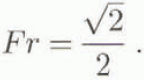
In the second phase, the front velocity is not constant but decreases. The height of the gravity current h is seen as constant along its full length but it decreases with time. The front is assimilated to a hydraulic jump and, if u _f indicates its velocity, the authors obtained

(7)

From the box model collapse of a two-dimensional gravity current of initial volume A ₀, Reference Hallworth, Phillips, Huppert and Sparks.Hallworth and others (1996) determined the time evolution of the length of the gravity current by

(8)

where the Froude number depends on the flow regime. They studied the entrainment of ambient fluid into the head of a gravity current propagating along a horizontal surface. The experimental technique relies on the neutralization of an alkaline current by entrainment of acidic ambient fluid. From dimensional analysis, they showed that the propagation of ambient-fluid entrainment into a gravity-current head depends only on the initial volume and distance from the release point. This result has been confirmed by their experimental results.

Physical Modelling and Experiments

In order to analyse the internal dynamics of gravity currents, we performed experiments on a scale model. Our experiments were undertaken in a horizontal flume 8.5 m long, 0.3 m wide and 0.5 m high (Fig. 1). A gate situated 0.30 m from one extremity contains the initial saline solution. The gate does not disturb the flow of the dense solution because it can be opened very rapidly. Fhe flume lateral walls are made of Plexiglas and meshed horizontally and vertically in order to examine the flow. The salt concentration is determined using a potentiomelric method. It consists of measuring the difference in potential between a reference electrode (whose potential depends only on temperature) and an electrode placed in the flow. The main merit of this method is the relatively high frequency of measurement. It is possible to obtain more than ten potential data per second. Such frequencies cannot be attained using a pH or conductimetry method.

Fig. 1.

Experimental flume.

An optical device was used to determine the internal velocity profiles. This makes it possible to examine particles using a light sheet about 1 cm thick. PVC particles are introduced into the initial saline solution in very small quantities in order to obtain some traces in the images. For each image, the camera stays open 1 second. The images are then digitized and processed by computer. The trace of each particle is then obtained and its velocity determined.

After the gate opens, the density gradient produces a motion that evolves rapidly into a developed gravity current. The flow rapidly takes a stable form with a head (lobes, fissures and whirls) and a body that spreads upstream. The whirls generate an incorporation of the ambient fluid through the interface. Near the ground the friction raises the front.

Numerical Modelling

In this section, the gravity current is considered to be a two-phase flow of a heavy fluid in a light fluid. The proposed model assumes that both fluids are Newtonian and that the solution does not modify either the behaviour of the fluid or the turbulence of the flow. The equations are written in a Galilean coordinates system formed by three axes: X and Y are in the horizontal plane (X is the flow direction) and Z is upward vertical, tn this coordinate system, the gravity vector is given by . The other variables are: ρ the density of the ambient fluid, the velocity vector, p the pressure and c the particle volumetric concentration.

The equations governing this kind of flow are the fluid-mechanics conservation laws. They are the conservation of air mass, conservation of salt or particle mass and momentum conservation. The introduction of Reynold’s decomposition followed by statistical processing produces the average equations of the mean flow. In these equations some new variables appear. They correspond to the second-order correlation resulting from the non-linearity of the Navier–Stokes equations. We determine them using the Boussinesq law which belongs to the class of models using the turbulent-viscosity concept. The equations of motion can be written as follows

(9)

The scale of the large turbulent eddies can be represented by the height of the gravity current.The turbulent viscosity is then linked to the kinetic turbulent energy k by the formula where L is the height of the gravity current. The turbulent-energy dissipation is then given by and the turbulent-energy production is given by

The calculation area is decomposed using an unstructured mesh into cells of variable dimensions. The equation system is written in the conservative form for its numerical resolution. The scheme is carried out in finite volumes. That allows good adaptation to an area of variable shape (relief of an avalanche path). The system is integrated on each cell between two consecutive times. The scheme is obtained in two steps. The projection step consists in allocating to each cell the average value of the vector and the integration step consists in integrating the system on each cell between times t ⁿ and (t ⁿ⁺¹. The Ostrogradsky theorem transforms the volumetric integral into a surface integral. Using the average values of neighbouring cells, we build the U gradient in older to obtain its linear approximation. For calculation of the diffusion terms we use the U gradient. On the other hand, for calculation of the hyperbolic part of the equation system and in order to preserve the stability of the scheme, it is necessary to limit the gradient value of U on each element in order to avoid new local extrema. It is important to notice here the limitation of the time-step introduced using the explicit scheme. The scheme is of second-order accuracy in space and first-order accuracy in time. The model needs a set of boundary conditions near the ground where the flow is considered to be a turbulent boundary layer defined by friction velocity and roughness.

Experimental Results

The aim of our experiments was to obtain velocity and concentration profiles within a gravity current for different initial conditions, in order to understand the internal dynamics of this kind of flow and also to test the validity of the numerical model for reproducing the internal variations of the concentration and velocity.

We installed six probes at different distances from the gate. They were placed 25, 100, 200, 300. 450 and 600cm from the gate. These sensors were placed vertically 2 cm abov e the bottom. At 100 cm from the gate, we placed two other probes vertically at 6 and 15 cm above the bottom. Four initial heights of the saline solution were tested: 10, 15, 20 and 30 cm. For all these tests the height of water was taken equal to the height of the saline solution. The following densities were studied: 1.013. 1.018, 1.021, 1.025, 1.029, 1.030, 1.038, 1.039, 1.041, 1.045, 1.049 and 1.053 Mgm ⁻³.

Using the results of all these experiments, it is possible to observe changes in density at different distances from the gate and also its vertical variations. The gravity currents have two siages. When the gate opened, we observed a rapid movement, follow ed by a flow with a constant front velocity. It is the slump regime. For this stage, the initial conditions are very important. In the second stage, inertia–buoyancy regime, the flow decelerated. In the first regime, the ambient fluid entrainment was negligible and the second regime was characterized by important water incorporation (Reference Hallworth, Phillips, Huppert and Sparks.Hallworth and others (1993)). The transition distance x _s is given by Equation (5).

Front Velocity

The velocity and position of the front of the gravity current are not the subject of this study. However, with the measured concentration peaks, it was possible to determine the mean front velocity by dividing the distance between successive probes by the difference between the arrival times at the probes. It was interesting to compare the results obtained with the earlier studies.

In Figure 2, we compare our experimental front velocities with those obtained using the theoretical Reference Huppert and SimpsonHuppert and Simpson (1980) model, for two different initial densities 1.018 and 1.041 Mg m⁻³. From this figure, we observe that when the front position x _f is less than x _s our results differ from the velocities computed by the above model. In the second regime, our results show a better fit.

Fig. 2.

Front velocity determined experimentally and computed using the Reference Huppert and SimpsonHuppert and Simpson (1980) model for two initial densities: 1.018 and 1.041 Mg m^−3.

Density Evolution in Time

The flow produced consists of a head and a body. If we observe variations in density at different fixed points, we can understand better the dynamics of the front and distinguish the behaviour of the front in different regimes. In Figure (3) the density evolution in time at 25, 200, 300, 450 and 600 cm from the gate is shown. The initial conditions were; height of the saline solution at 20 cm, the water height at 20 cm and density at 1.025Mg m⁻³. First of all and for the every curve, we observed a density peak followed by a decrease and finally a stable state. We noticed that the maximum density was always found at the front of the flow. This maximum value decreased with the distance covered (x _f) and this decrease was very low if x _f was less than x _s. If we looked carefully, we observed that the peak possessed a certain length which decreased with the distance covered. Subsequently, it seems reasonable to assume that the length of the concentration peak, where the density is equal to the initial density, represents the length of the head. When we computed this length, we obtained 65 cm for the probe placed 25 cm from the gate where the measured front velocity was equal to 13 cm s⁻¹. For all the tests, we determined an empirical power law for the time evolution of the maximum front density. It is given by

(10)

where ρ _max is the front maximum density, ρ _a is the ambient fluid density, ρ ₀ is the initial density of the saline solution, g is the gravity acceleration and t the time. This empirical law is plotted in Figure 3.

Fig. 3.

Density variation in time for initial density of 1.025 Mg m⁻³, where initial saline-solution height is 20 cm, initial water height is 20 cm and probes placed at 25, 200, 300, 450 and 600 cm from the gate and 2 cm from the bottom.

In the following analysis the dimensionless variables below will be used:

(11)

(12)

(13)

(14)

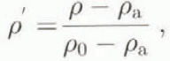
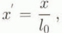
Figure 4 shows the variations in time of dimensionless densities obtained for initial densities equal to 1.013, 1.018, 1.032 and 1.041 Mg m⁻³ and x _s = 300 cm. In this figure, the probe has been placed 25 cm from the gate and 2 cm vertically above the bottom. We notice that the maximum density at this point is almost equal to the initial density.

Fig. 4.

Time variations of dimensionless density at x equal to 25 cm from the gate corresponding to the slump regime of the gravity current on a horizontal bottom and for initial densities of 1.013, 1.018, 1.032 and 1.041 Mg m ⁻³ and x_s equal to 300 cm.

Figure 5 shows the variations in time of dimensionless densities, obtained for initial densities of 1.013, 1.032 and 1.038 Mg m⁻³ and x _s = 300 cm, in the ease of a probe placed 600 cm from the gate. For all these cases, the probe is located more than x _s from the gate. We notice that the maximum density reached is below the initial density. In all these curves the maximum density is often less than 60% of the initial density. We can then conclude that beyond this distance entrainment becomes important and the front density decreases fast.

Fig. 5.

Time evolution of dimensionless density at 600 cm corresponding to the inertia–buoyancy of a gravity current on a horizontal bottom. The initial densities are 1.013, 1.032 and 1.038 Mg m⁻³ and x_s = 300cm.

Figure 6 shows the variations in time of dimensionless densities obtained for initial densities of 1.018, 1.032 and 1.041 Mg m⁻³ for a probe placed 200 cm from the gate. The distance between the probe and the gale is equal to a value of x _s (x _s = 200 cm). It is the transition zone where the maximum density is about 80% of the initial density.

Fig. 6.

Time evolution of dimensionless density at 200 cm corresponding to the transition regime of a gravity current on a horizontal bottom. The initial densities are 1.018, 1.032 and 1.041 Mg m⁻³ and x_s = 200 cm.

Figures 4, 5 and 6 show dimensionless density evolution respectively, corresponding to the slump zone, the transition zone and the inertia–buoyancy zone.

Front-Concentration Analysis

For all our experiments we determined the front density as a function of the distance covered and also the slump distance x _s, which is the distance after which we can identify the beginning of the significant mixing. Reference Hallworth, Phillips, Huppert and Sparks.Hallworth and others (1993) determined empirically the entrainment ratio r as a function of y(y = x _f − x _s) by

(15)

The dimensionless density can be linked to this ratio r by

(16)

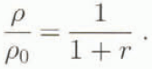
In Figure 7 we have plotted our measurements and compared them to the Hallworth law. For y < 0, the maximum density according to the distance covered, in our experiments, is often equal to the initial saline density. We can then confirm that before the from reaches a distance x _s, air entrainment is negligible. For y > 0, the maximum density decreases and evolves towards the Hallworth law.

Fig. 7.

Measured maximum front density divided by the initial density as a function of (yA₀ ^−0.5) for all data from two-dimensional constant-volume currents moving over a horizontal bottom.

Vertical Density Profiles

The probes placed vertically at x = 100 cm from the gate allowed us to determine for each experiment the density evolution according to time at three heights from the bottom (2,6 and 15 cm). From Figure 8, obtained for an initial density of 1.039 Mg m⁻³ and h ₀) = H = 30 cm. we can show that when the current arrives at x = 100 cm the density ai z = 2 cm reaches a value equal to the initial density, and the probe placed 6 cm from the bottom reaches a value of about 70% of the initial density. After passage of the peak, we observed that the probes placed at 2 and 6 cm recorded almost the same density. The density evolution obtained at z = 15 cm shows a lower density. The vertical density profiles, obtained at different steps of the flow, show that the concentration decreases upwards vertically. This decrease is smaller in the transition zone between the head and the body. In this zone, the vertical distribution of the density is quasi-uniform in the lower part of the flow.

Fig. 8.

Density evolution as a function of time at 100 cm from the gate and for three different distances above the bottom (2, 6 and 15 cm). The initial density is 1.039 Mg m⁻³, initial height of saline solution is 20 cm and the initial water height is 20 cm.

Velocity Measurements

From some images, we could establish the velocity profile within the flow. In Figure 9 we show the experimental profiles obtained for an initial density of 1.009 Mg m⁻³, h ₀ = 20 cm and H = 20 cm at x _f = 110, 120, 130, 140 and 150 cm from the gate. These profiles are shown in Figure 10 and allowed us to define the structure of the flow in the front and in the body of the slump regime.

Fig. 9.

Velocity profiles obtained at different dislances from the gate in the case of a constant-volume gravity current of initial density 1013 Mg m⁻³ and h₀ = H = 20 cm.

Fig. 10.

Structure of the head of a gravity current in the slump regime obtained using the velocity profiles of Figure 9.

Comparison between Numerical and Experimental Results

A comparison between the numerical and experimental results will be undertaken in order to show the ability of the numerical model to reproduce the experimental results. The first comparison concerns the evolution of the density as a function of the time at different distances from the gate. Figure 11 shows the experimental and numerical densities at x = 100 cm and x = 200 cm, in the case of an initial density of 1.038 Mg m⁻³, H = 20 cm and h ₀ = 20 cm. The arrival time and the front density are very well reproduced by the model. In the transition zone between the front and the body, the numerical results are smoothed and do not agree very well with the experimental results. The density evolution in the body is reproduced well. For greater distance from the gate, the numerical results agree well with the experimental results.

From the same test, and using the probes placed vertically the same distance from the gate, we can test the numerical model for reproducing variations in the vertical distribution of the density. In Figure 12, we show this comparison and can conclude that the density peak and its arrival time is reproduced well but also note that the numerical results are smoothed.

Fig. 11.

Numerical and experimental density profiles at 100 and 200 cm from the gate in the case of initial density of 1.038 Mg m⁻³ H = 20 cm, h₀ = 20 cm.

Fig. 12.

Numerical and experimental time–density evolution in the case of initial density of 1.038 Mg m⁻³, H = 20 cm, h₀ = 20 cm at different heights from the bottom (2.6 and 15 cm) at x = 100 cm from the gate.

Concerning the velocity profiles and for x = 110 cm from the gate (slump zone), we can show i see Fig. 13) that the numerical model profiles are close to the experimental ones. The lower part of the head of the current, where the velocity is positive, represents more than 60% of the height (h) of the head. The vorticity centre is situated at 0.7 h and the positive velocity in the lower part is greater than the negative velocity in the upper region.

Fig. 13.

Numerical and experimental velocity profiles at x_f = 110 cm and t = 12 s obtained in the case of two-dimensional constant-volume gravity currents on a horizontal bottom for the following initial density = 1.013 Mg m⁻³, initial height of the saline solution = 20 cm and height of the water = 20 cm.

Conclusion

Earlier theories and experiments concerning gravity currents contain a great deal of information about front dynamics in terms of velocity, height and ambient-fluid entrainment. The novelty of this paper resides in its analysis of the structure of the front of the gravity current using measurements of internal concentration and velocity profiles. This analysis was performed using an experimental device and a numerical model for the Navier–Stokes equations. We obtained measurements of the concentration within tin-gravity current using potentiometric sensors and also the velocity using image-processing techniques. We have analysed front dynamics and confirmed the existence of two important stages. The two parts behave quite differently. For x _f < x _s, where the dynamics depend on the initial conditions, where the flow consists of a head and body, and the front density is constant. For x _f > x _s, we show that the density of the front decreases and evolves towards the Hall-worth and others (1993) law. From a comparison between the experiments and the numerical model results, we show that this kind of model can predict well the flow in the slump regime and in the inertia–buoyancy regime with smoothed results in the transition from the head to the body of the gravity current.