





1 Introduction
We formalize the process by which a researcher uses fixed factor-loading thresholds (say, loadings
$\le 0.30$
 ) to delete items. This study provides insight into the process and suggests an alternative strategy that retains all items while weighting them in such a way that each item contributes to increasing reliability compared to deleting the item, when its weight would be zero. Many of our derivations are based on assuming congeneric items, and we focus on total-score reliability, but we also generalize some results to non-congeneric, multifactor contexts. To isolate the phenomena of interest, we ignore the fact that many additional criteria may be considered when constructing a test, such as content validity and interrater reliability.
Two rules of thumb that are frequently used to delete items in test construction are:
-
1. The fixed loading threshold rule: Remove items with factor loadings less than 0.30 (or some other fixed value).
-
2. The alpha contribution rule: Remove items if alpha-if-item-deleted (AIID) is greater than the coefficient alpha.
We refer to alpha because it is popular among researchers, but our theoretical developments use the formal reliability definition (Lord & Novick, Reference Lord and Novick1968, p. 61), independent of the method used to estimate reliability.
The two rules of thumb are closely related because, in unifactorial item sets, items with a low loading often have a low or negative contribution to coefficient alpha (see Section 2, where we discuss the rules of thumb in more detail). However, theoretical support for the fixed loading threshold is virtually nonexistent. In this article, we develop alternative thresholds for factor loadings, based on the idea that each item should contribute positively to reliability. An advantage of the new thresholds is that, unlike the fixed loading threshold rule, they are clearly motivated and rigorously derived from a model. A second advantage is that they are more generally applicable than the alpha contribution rule. Thus, we improve both rules but recognize that when one adopts a broader perspective of test improvement, reliability is just one of the various considerations to realize this goal. Focusing on reliability, removing an item means that the item gets scoring weight zero in the total score, and therefore we also investigate the more subtle alternative of giving such items a smaller but positive weight. We performed a computational study to support the theoretical results and obtained robustness results for multiple factors. A real-data example illustrates the applicability of the various methods.
Because of our theoretical perspective, we impose three limitations on this study, of which we already mentioned two: Firstly, we assume congeneric items that we consider also valid indicators of the intended attribute, so that they are interchangeable to a high degree. Secondly, we focus on reliability rather than a specific method for estimating reliability. The third limitation refers to studying the population covariances between items; then, exploratory and confirmatory factor analysis should yield identical factor loadings, so that for our theoretical results, it is immaterial whether the factor analysis is confirmatory or exploratory.
2 Literature review
In this section, we review literature recommending the loading threshold, we explore the origins of the loading threshold, and we discuss some criticisms. Next, we discuss the alpha contribution rule and its relationship to the loading threshold. We also discuss how our approach relates to the estimation of factor scores.
2.1 The fixed loading threshold rule
Researchers’ practical use of loadings to add items to or delete items from a test is rather informal and flexible. Loading lower bounds may vary between studies or within one study. Sometimes a fixed number of items having the lowest loadings are removed to realize a desired test length shorter than the original test length to ease the burden to test takers, such as patients and young children. Kruyen et al. (Reference Kruyen, Emons and Sijtsma2013) found that researchers regularly and flexibly use loadings to remove items. We focus on the much-used rule to remove (select) items having loadings below (above) some fixed threshold.
We mention a few examples of psychometricians’ recommendation that factor loadings should be at least 0.30 (or another value) for item inclusion: the COnsensus-based Standards for the selection of health Measurement Instruments (COSMIN, n.d., p. 2); also, see Clark and Watson (Reference Clark and Watson1995, p. 317), Costello and Osborne (Reference Costello and Osborne2005, p. 4), Field (Reference Field2009, pp. 645, 666), Floyd and Widaman (Reference Floyd and Widaman1995, pp. 294–295), Howard (Reference Howard2016, p. 55; Reference Howard2023), Izquierdo et al. (Reference Izquierdo, Olea and Abad2014, p. 397), Nunnally (Reference Nunnally1978, p. 422), Samuels (Reference Samuels2017, p. 1), and Tabachnick and Fidell (Reference Tabachnick and Fidell2001, p. 625; Reference Tabachnick and Fidell2013, p. 654). The earliest source we traced is Nunnally (Reference Nunnally1978), who already described it as “an old rule.” The motivations for the rules these authors provided can be grouped as follows:
-
1. A loading of 0.30–0.40 corresponds to 9%–16% explained variance (Nunnally; Tabachnick & Fidell; Field).
-
2. Low loadings imply only modest correlations with other variables (Clark & Watson).
-
3. Low loadings are nonsignificant or unstable (Floyd & Widaman; Samuels).
-
4. The empirical distribution of the smallest primary loading based on meta-analysis (Howard, Reference Howard2023).
-
5. Reference to a secondary source, repeating the rule without motivation (Costello and Osborne; Howard, Reference Howard2016).
-
6. No motivation and no reference (COSMIN; Izquierdo et al.).
Only four of the eleven cited sources (COSMIN; Samuels; Clark & Watson; Floyd & Widaman) suggest removing items with low loadings. The others recommend thresholds for interpreting factors, not for removing items. Most sources concern exploratory factor analysis (EFA).
These motivations are not convincing. Motivations (1) and (2) are merely restatements of the cutoff in different metrics, and motivation (3) depends strongly on sample size. Motivation (4) summarizes common practice but does not justify it. The sources in (5) cite either one of the sources in (1)–(4) or a source unavailable to us. Several authors have argued that loading thresholds are subjective and arbitrary and should depend on the attribute (Howard, Reference Howard2023, pp. 5, 9–10; Ondé & Alvarado, Reference Ondé and Alvarado2020, pp. 2, 8; Tabachnick & Fidell, Reference Tabachnick and Fidell2013, p. 654). We conclude that there are no compelling reasons for a fixed loading threshold.
Interestingly, none of the cited authors mentions the possibility that removing items with low loadings affects total-score reliability. If a researcher pursues high reliability and uses a loading threshold, then the 0.30 loading threshold may have an adverse effect. In some domains, such as evoked response potentials (ERPs), items may be highly similar and almost parallel, but single-item reliability is low yielding factor loadings ranging from 0.10 to 0.20. Yet, using many items, the Spearman–Brown formula implies that scale reliability can still be high. For example, unifactorial items with a loading of 0.20 have a reliability of 0.04, and a test of 100 of such items has a composite reliability of 0.81. Use of the 0.30 loading threshold would result in the deletion of all items, which is clearly an incorrect decision. Strict adherence to the 0.30 loading threshold may result in the opposite result of what the researcher pursues. The example of items with loadings of 0.20 suggests that it is not the absolute size of the loading that matters but its loading relative to the other items. We therefore investigated whether we could formulate a simple rule of thumb that uses the ratio of an item’s loading to other loadings to predict its contribution to reliability.
As an aside, a recommendation related to the loading threshold in the context of classical test theory is the requirement that the correlation of the item with the total score leaving out the item under consideration exceeds a certain threshold (e.g., Evers et al., Reference Evers, Lucassen, Meijer and Sijtsma2019). For many congeneric items with approximately equal loadings, the total score correlates highly with the underlying factor, so that the criterion that the (corrected) item-total correlation exceeds a certain threshold is almost equivalent to the criterion that the factor loading exceeds some (slightly different) threshold. Therefore, we do not discuss a fixed corrected item-total correlation threshold as a separate rule of thumb.
2.2 The alpha contribution rule
The alpha contribution strategy entails computing coefficient alpha (e.g., Sijtsma & Pfadt, Reference Sijtsma and Pfadt2021) for the total set of items and computing it again after one of the items is removed, resulting in
$AIID$
 ; if
$AIID> alpha$
 , the item is deleted because of its negative contribution to reliability. Raubenheimer (Reference Raubenheimer2004) discussed an application of AIID to Allport and Ross’ (Reference Allport and Ross1967) Religious Orientation Scale. AIID has been criticized because it can impair construct validity (Cho & Kim, Reference Cho and Kim2015) and criterion validity (Raykov, Reference Raykov2008). We concur, but study congeneric items to be able to control the formalization of the process. In their survey, Hoekstra et al. (Reference Hoekstra, Vugteveen, Warrens and Kruyen2019) found that most researchers hesitated to remove an item if that would increase alpha. We notice that because alpha is not necessarily equal to the reliability when items are not essentially tau-equivalent (Lord & Novick, Reference Lord and Novick1968, p. 50), reliability results may be misleading, but this is not a problem typical of alpha. An item with a relatively large error variance can lower composite reliability, regardless of how it is estimated.
2.3 Empirical examples of the relation between loadings and alpha contributions
To illustrate the relation between factor loadings and alpha contribution with data from the literature, we analyzed the data made available by Dragostinov and Mõttus (Reference Dragostinov and Mõttus2022) for the 27 items of the Short Dark Triad questionnaire at time 1. Three related factors underlie this questionnaire. We nevertheless estimated the factor loadings with the maximum likelihood method in a one-factor model. Figure 1 shows that there is a strong correlation between factor loadings and corrected item-total correlations (r = 0.96) and between factor loadings and AIID (r = −0.97). This result is typically found in other datasets as well. For the 20-item Driving Cognition Questionnaire in the dataset of Fischer et al. (Reference Fischer, Schröder, Taylor and Heider2023), we found r = 1.00 and r = −0.99; and for the 10-item scales of the Adjective Checklist in the dataset “acl” of the R package “mokken” (van der Ark, Reference van der Ark2012), restricted to the six scales that have RMSEA < 0.10 in an ML-factor analysis with one factor, we found mean correlations of 0.98 between loadings and item-rest correlation and −0.98 between loadings and AIID. For the other scales of this dataset, with RMSEA > 0.10, correlations could be as low as 0.80 and −0.76. The high correlations should not surprise us, because in a linear one-factor model, the corrected item-total correlations and AIIDs are completely determined by the factor loadings and the item variances. Therefore, in this article, we will study the effect of the factor loadings and item variances on reliability.
Relationships between factor loadings and corrected item-total correlations (left) and alpha-if-item-deleted (right) for the same data.

Figure 1. Long description
The image consists of two side-by-side scatter plots with orange data points.
Left Panel: Corrected Item-Total Correlation.
- The horizontal X axis is labeled Factor loading with values from 0.00 to 0.80.
- The vertical Y axis has values from 0.00 to 0.60.
- The data points show a strong positive linear increase. As factor loading increases from approximately 0.15 to 0.65, the corrected item-total correlation increases from approximately 0.18 to 0.58.
Right Panel: Cronbach's Alpha if Item Deleted.
- The horizontal X axis is labeled Factor loading with values from 0.00 to 0.80.
- The vertical Y axis has values from 0.83 to 0.84.
- The data points show a strong negative linear trend. As factor loading increases from approximately 0.15 to 0.65, the alpha-if-item-deleted value decreases from approximately 0.84 to 0.83.
2.4 Optimal weighting, factor scores, and item removal
Raykov (Reference Raykov2024) defines the optimal linear combination (OLC) of item scores as the linear combination that maximizes reliability. For congeneric items, the optimal scoring weight of the ith item is given by
${\beta}_i/{\varepsilon}_i^2$
 , where
${\beta}_i$
 is the factor loading and
${\varepsilon}_i^2$
 is the item’s unique variance (Conger, Reference Conger1980, p. 371; Jöreskog, Reference Jöreskog1971, p. 112; Raykov, Reference Raykov2024, p. 997). If the items are standardized, this expression reduces to
${\beta}_i/\left(1-{\beta}_i^2\right)$
 .
Alternatively, one may estimate factor scores with Thurstone’s least squares regression method (Grice, Reference Grice2001). For standardized items with correlation matrix
$\mathbf{R}$
 and structure matrix
$\mathbf{S}$
 (the correlations between the factors and the items), the matrix of factor-score coefficients
$\mathbf{W}$
 is given by
$\mathbf{W}={\mathbf{R}}^{-1}\mathbf{S}$
 (Grice, Reference Grice2001, p. 433). For congeneric items, applying the Sherman–Morrison formula (Bartlett, Reference Bartlett1951, Equation (2)) to obtain
${\mathbf{R}}^{-1}$
 , this yields the scoring weight for item
$i$
 as

where
$V=\sum \limits_j{\beta}_j^2/\left(1-{\beta}_j^2\right)$
 (see the Supplementary Material for a detailed derivation: https://osf.io/5nmr9). Hence, for congeneric items, the OLC equals the Thurstone factor scores up to the multiplicative constant
${\left(1+V\right)}^{-1}$
 .
In the following sections, we show that for congeneric items, adding a new item always increases the reliability of the total score, provided that the item is assigned a sufficiently small weight in the computation of the total score. In other words, instead of deleting an item, scale reliability may increase by assigning a smaller weight to the item. Since removing an item is equivalent to assigning it a weight of zero, it is logically impossible to increase the reliability of the OLC by removing an item. At first glance, our conclusion that items should be weighted rather than deleted may therefore seem trivial. However, our results do not only apply to the OLC but to any linear combination with positive weights. We introduce a strategy that assigns sufficiently small positive weights; the weights need not be optimal. This is relevant because test constructors may prefer to use unit weights for most items and adjust weights only for items that make a negative contribution to reliability under unit weighting. One motivation for this approach is that estimated optimal weights are not always superior to unit weights in finite samples (e.g., Grice, Reference Grice2001, p. 434; Sijtsma et al., Reference Sijtsma, Ellis and Borsboom2024). Using unit weights for most items and reduced weights for some items may thus represent a compromise between the methods of unit-weight scoring and fully optimal scoring. Consequently, our aim to develop a rule of thumb for identifying items with negative reliability contribution remains relevant.
3 Notation, assumptions, and definitions
Let the items be random variables, numbered
$1,2,\dots, n$
 , and let the corresponding observed-score variables be
${X}_1,{X}_2,\dots, {X}_n$
 . We assume that there are corresponding true-score variables
${T}_1,{T}_2,\dots, {T}_n$
 , for which we define the error-score variables
${E}_1,{E}_2,\dots, {E}_n$
 as
${E}_i={X}_i-{T}_i$
 for
$i=1,\dots, n$
 . We assume furthermore that
$Cov\left({E}_i,{T}_j\right)=0$
 for
$i,j=1,\dots, n$
 , and
$Cov\left({E}_i,{E}_j\right)=0$
 for
$i,j=1,\dots, n;i\ne j$
 . We assume that all these variables have finite variances, and we denote the following shorthand notations for the item variances and reliabilities:


and

We assume
${\tau}_i^2>0\;\mathrm{for}\kern0.17em \mathrm{each}\kern0.17em \mathrm{item}\;i=1,\dots, n.$
 We will consider the reliability of weighted sum scores. Such weighted sum scores can be written as
${\pi}_1{X}_1+{\pi}_2{X}_2+\dots +{\pi}_n{X}_n$
 , where the
${\pi}_i$
 s are real numbers that we will call scoring weights. An example with a test of four items would be if a researcher computes total scores as
$3.1{X}_1+2.7{X}_2+1.6{X}_3+0.6{X}_4$
 . We will also consider sum scores based on subsets of the total set of
$n$
 items and call them partial sum scores. To keep different partial sum scores on comparable scales, we will divide all sum scores we discuss by the sum of the weights and thus obtain weighted mean scores. In the previous example, the weighted mean scores would be
$\left(3.1{X}_1+2.7{X}_2+1.6{X}_3+0.6{X}_4\right)/\left(3.1+2.7+1.6+0.6\right)$
 . In general terms, we assume that there is some set of scoring weights
${\pi}_1,\dots, {\pi}_n\in \mathbb{R}$
 , chosen a priori, and for any subset of items
$A\subseteq \left\{1,\dots, n\right\},$
 we define the weighted mean scores as


Furthermore, we define for this item subset


and

We will give special attention to the case where all
${\pi}_i$
 s are equal to 1, which leads to the total score
$\sum \limits_{i=1}^n{X}_i/n$
 , which we call the simple mean score or unweighted mean score. The terms total score or test score will henceforth be used for any of the weighted sum scores delineated above.
We say that the items are congeneric (or unifactorial) if there is a variable
$T$
 such that for every item
$i=1,\dots, n$
 , there are scalars
${\beta}_i,{\gamma}_i\in \mathbb{R}$
 , with
${\beta}_i>0$
 , such that
${T}_i={\beta}_iT+{\gamma}_i$
 . We use the term loadings for the
${\beta}_i$
 . We say that the items are essentially tau-equivalent if they are congeneric with
${\beta}_i=1$
 , so that
${T}_i=T+{\gamma}_i$
 . We say that the items are tau-equivalent if
${T}_i=T$
 for all
$i=1,\dots, n$
 , and in this case, we write
${\tau}_i^2={\tau}^2$
 .
It is important to distinguish the scoring weights
${\pi}_i$
 from the loadings
${\beta}_i$
 . The loadings are determined by the data, because for congeneric items, we have
$Cov\left({X}_i,{X}_j\right)={\beta}_i{\beta}_j$
 . The scoring weights, on the other hand, are the weights that are used by the test user when a total score is computed for each subject. These weights are usually chosen by the test developer and prescribed in the test manual, but they need not have any relationship with the loadings. A few examples are: (1) more often than not, a simple mean score is used as the test score, regardless of the loadings (e.g., Sijtsma et al., Reference Sijtsma, Ellis and Borsboom2024); (2) a teacher may decide to emphasize essay questions more than multiple-choice questions because they require more time to answer; and (3) computing the mean of standardized item scores, with each item’s scoring weight equal to the reciprocal of its standard deviation.
Although factor loadings do not necessarily influence scoring weights, such influences are not uncommon either. For example, Guilford (Reference Guilford1941) argued that scoring weights should be regression coefficients. If the test developer decides to estimate factor scores, the scoring weights will be influenced by the loadings. In principal component analysis, the scoring weights for the first principal component are proportional to the loadings on the first principal component, but in other forms of factor analysis, the scoring weights are usually not proportional to the factor loadings; hence, distinguishing the concepts of scoring weights and factor loadings remains important. With this distinction in mind, our research questions become
-
1. Given the factor loadings, which restrictions should the scoring weights satisfy to increase the reliability of the total score when a new item is added?
-
2. Given the scoring weights, which restrictions should the factor loadings satisfy to increase the reliability of the total score when a new item is added?
4 If the test score is the weighted mean score
Consider two disjoint sets of items,
$A,B\subseteq \left\{1,\dots, n\right\};A\cap B=\varnothing$
 . Suppose that a subtest scoring weight
$\theta \in \left[0,1\right]$
 is used to create a weighted combination of subtest scores,

and let
$\rho \left(\theta \right)$
 be the reliability of
$X\left(\theta \right)$
 . Thus,
$X\left(\theta \right)$
 is the total test score obtained with new weights
${\pi}_i^{\prime }=\left(1-\theta \right){\pi}_i$
 if
$i\in A$
 and
${\pi}_i^{\prime }=\theta {\pi}_i$
 if
$i\in B$
 . The reliability of subtest A is
${\rho}_A$
 , the reliability of subtest B is
${\rho}_B$
 , and the reliability of their
$\theta$
 -weighted mean is
$\rho \left(\theta \right)$
 . For which
$\theta$
 is
$\rho \left(\theta \right)>{\rho}_A$
 ? That is, if we start with subtest A and extend it with subtest B, for which subtest scoring weight
$\theta$
 of subtest B will the reliability of the composite test exceed the reliability of the original subtest A?
Theorem 1.
If the items are tau-equivalent with
${\rho}_A<1$
 and
${\rho}_B>0$
 , then
$\rho \left(\theta \right)>{\rho}_A$
 if and only if

Proof. Because the items are tau-equivalent,
${T}_i=T$
 , and the item true-score variance equals
${\tau}_i^2={\tau}^2$
 . The subtest scores are weighted means of the item scores,
${X}_A=T+{E}_A$
 and
${X}_B=T+{E}_B$
 , which means that
${X}_A$
 and
${X}_B$
 are also tau-equivalent with each other. Then,
$X\left(\theta \right)=T+\left(1-\theta \right){E}_A+\theta {E}_B$
 , and

Hence, the error component of
$X\left(\theta \right)$
 is given by
$\left(1-\theta \right){E}_A+\theta {E}_B$
 , which has variance

Therefore,

We also know that

Then, comparing these two reliabilities,

is equivalent with comparing the error variances on both sides,

Note that we initially assumed
$\theta \ge 0$
 , and that
$\theta =0$
 would contradict the above inequality. After some algebraic manipulation we skip here, aimed at expressing
$\theta$
 in the other quantities, we obtain

Remark 1. The right-hand side is maximal if
${\varepsilon}_B^2=0$
 . Then, the theorem sets the bound
$\theta <2$
 , but
$\theta$
 was required to be in
$\left[0,1\right]$
 from the beginning. Thus, the theorem then says that
$\rho \left(\theta \right)>{\rho}_A$
 for all
$\theta \in \left(0,1\right]$
 .
Remark 2. The upper bound for
$\theta$
 can also be expressed in terms of the reliabilities of A and B. This can be done by first rewriting
${\rho}_A={\tau}^2/\left({\tau}^2+{\varepsilon}_A^2\right)$
 to
${\varepsilon}_A^2$
 , so that

and similarly, for
${\varepsilon}_B^2$
 , and then developing

until we obtain

Therefore, Theorem 1 can be rephrased as follows: If the items are tau-equivalent with
${\rho}_A<1 $
 and
${\rho}_B>0$
 , then the reliability of
$X\left(\theta \right)=\left(1-\theta \right){X}_A+\theta {X}_B$
 is greater than the reliability of
$\ {X}_A$
 if and only if

Remark 3. Under the conditions of Theorem 1, the reliability of the composite test with score
$X\left(\theta \right)=\left(1-\theta \right){X}_A+\theta {X}_B$
 is given by


Figure 2 shows how
$\rho \left(\theta \right)$
 depends on the subtest scoring weight
$\theta$
 for the case of reliabilities
${\rho}_A=0.5$
 and
${\rho}_B=0.1$
 . The reliability of the composite test (blue curve) exceeds the reliability of test A (orange line) only for
$0<\theta <0.2$
 . For larger weights
$\theta$
 , the reliability of the composite test comes closer to the reliability of test B and is smaller than the reliability of test A.
Relationship between
$\rho \left(\theta \right)$
 and
$\theta$
 for the case of reliabilities
${\rho}_A=0.5$
 and
${\rho}_B=0.1$
 , for the composite test (blue curve), test A (orange line), and test B (gray line).

Figure 2. Long description
The X-axis is labeled with the Greek letter theta, ranging from 0 to 1 in increments of 0.2. The Y-axis is labeled Reliability, ranging from 0 to 0.6 in increments of 0.1.
Three lines are plotted:
* Test A (orange line) is a horizontal constant at a reliability of 0.5.
* Test B (gray line) is a horizontal constant at a reliability of 0.1.
* Composite test (blue line) starts at 0.5 when theta is 0, rises slightly to a peak of approximately 0.53 near theta equals 0.1, and then follows a downward sigmoidal curve. It crosses the Test A line at theta equals 0.2 and continues to decrease until it meets the Test B line at a reliability of 0.1 when theta equals 1.
A legend at the bottom identifies the blue line as Composite test, the orange line as Test A, and the gray line as Test B.
Next, we discuss two corollaries. The first corollary is a qualitative rephrasing of Theorem 1, where we use a single item for subtest B, thus referring to the situation where we add one item at a time to the existing item set. Furthermore, we may replace the condition of tau-equivalence with essential tau-equivalence, since this does not affect the reliability.
Corollary 1. For essentially tau-equivalent items, adding a new item with positive reliability to an existing set of items with reliability less than 1 will increase the reliability of the weighted mean score if the scoring weight of the new item is positive and small enough.
The second corollary deals with the case where items are congeneric, but not necessarily essentially tau-equivalent. If the items are congeneric, and the items of B have positive reliability
${\rho}_i>0$
 , we can first multiply
${X}_B$
 with a factor
${\tau}_A/{\tau}_B$
 , which makes it essentially tau-equivalent with
${X}_A$
 . Next, we can apply Corollary 1. This leads to the following corollary.
Corollary 2. For congeneric items, adding a new item with positive reliability to an existing set of items with reliability less than 1 will increase the reliability of the weighted mean score if the scoring weight of the new item is positive and small enough.
Thus, for a congeneric item pool of items with positive item reliabilities, when one adds a new item from the item pool to the test, it is impossible that the new item decreases the reliability of the test per se; there is always a scoring weight for the new item that increases the reliability of the total score. Even if the new item has a very low reliability, including it in the test can still increase the reliability of the total score, provided that its scoring weight is small enough.
As discussed in Section 2.4, Jöreskog (Reference Jöreskog1971) and Conger (Reference Conger1980) showed that, for congeneric tests, the reliability of the weighted mean score is maximized with scoring weights
${\pi}_i={\beta}_i/{\varepsilon}_i^2$
 (see also Ogasawara, Reference Ogasawara2009; Raykov, Reference Raykov2024; Wang, Reference Wang1998). Using these scoring weights, we obtain the OLC. Raykov (Reference Raykov2024) notes that, logically, the reliability of the OLC cannot be lower than the reliability of the simple mean (i.e., with
${\pi}_i=1/n$
 ). Similarly, the reliability of the OLC cannot be lower than the reliability of the simple mean with one item removed (i.e., with
${\pi}_i=1/\left(n-1\right)$
 for
$i=1,\dots, n-1$
 , and
${\pi}_n=0$
 ). Denote this latter reliability by or
$\rho_{n-1}$
 ${\rho}_{\left\{1, \dots, n-1\right\}}$
. Now assume that
${\beta}_i>0$
 and that the reliability of the OLC is strictly greater than
${\rho}_{\left\{1, \dots, n-1\right\}}$
 , which is probably the most common situation. This means that the optimal scoring weights with
$n$
 items outperform the simple scoring weights with
$n-1$
 items, but it does not address what happens to the reliability when item
$n$
 is added under non-optimal scoring weights. Corollary 2 says that, regardless of the scoring weights used for the first
$n-1$
 items, there exists an entire interval of scoring weights for item
$n$
 that will increase reliability. Several authors have pointed out that estimates of optimal weights in finite samples may be far from optimal (Aguirre-Urreta et al., Reference Aguirre-Urreta, Rönkkö and McIntosh2019; Sijtsma et al., Reference Sijtsma, Ellis and Borsboom2024), and Corollary 2 suggests that other weights (neither optimal nor simple) may still improve reliability.
5 If the test score is the simple mean score
5.1 The case of equal error variances
We now consider
$A=\left\{1,\dots, n-1\right\}$
 and
$B=\left\{n\right\}$
 . We consider the simple (unweighted) mean score across items, that is,
$\sum _{i=1}^n{X}_i/n.$
 For the first
$n-1$
 items, we define

Next, we introduce Theorem 2, which sets a lower bound to
${\beta}_n$
 relative to the mean of the
$n-1$
 ${\beta}_i$
 s already in the preliminary test defined by set
$A$
 . We prove that this lower bound needs to be satisfied if we require the reliability of the
$n$
 items to exceed the reliability of the
$n-1$
 items in
$A$
 . In this and other proofs, some intermediate steps were first identified using Symbolab (www.symbolab.com). However, all steps were thoroughly checked by the authors and can be reproduced through elementary, though sometimes tedious, algebra or calculus.
Theorem 2.
Assume the items are congeneric and that their error variances are equal, say
$\ {\varepsilon}_i^2={\varepsilon}^2$
 , and that the simple mean score is used as the test score. Then
${\rho}_{\left\{1,\dots, n\right\}}>{\rho}_{\left\{1, \dots, n-1\right\}} $
 if and only if

Proof. Without loss of generality, we can set
$Var(T)=1$
 . Then, summing across the mean score of the items in
$A$
 ,
$i,j\in \left\{1,\dots, n-1\right\}$
 , we derive

Next, we add item
$n$
 and derive

The error variance for the items in
$A$
 is

and the error variance for the items in
$A$
 and item
$n$
 together is

Now, we demand that the reliability of the
$n$
 -item test is greater than the reliability of the
$\left(n-1\right)$
 -item test and derive a quadratic function in
$\frac{\beta_n}{\overline{\beta}}$
 . That is, we develop the inequality as follows:


Simplifying the final inequality in a couple of steps that we skip here, we obtain the quadratic equation we were looking for, and which enables us to put a lower bound on
$\frac{\beta_n}{\overline{\beta}}$
 . The equation derived from
${\rho}_{\left\{1,\dots, n\right\}}>{\rho}_{\left\{1,\dots, n-1\right\}}$
 is

Solving the quadratic equation

in
$\frac{\beta_n}{\overline{\beta}}$
 yields (derived with the help of Symbolab)

The admissible solutions are only with
$\frac{\beta_n}{\overline{\beta}}>0$
 ; therefore, we have

Proposition 1.

Proof (derived with the help of Symbolab).

Furthermore, notice that
$1-n+\sqrt{n\left(n-1\right)}$
 increases in
$n$
 , so that the limiting value we just derived defines an upper bound for the lower bounds
$\frac{\beta_n}{\overline{\beta}}$
 if our goal is to increase reliability when selecting item
$n$
 . Thus, we have come to the following result:
For congeneric items with equal error variances, if the unweighted mean score is used as the test score, and for any test length
$\ n-1$
 , if the next item, say, item
$n$
 satisfies

then
${\rho}_n>{\rho}_{n-1}$
 .
Contrary to the common rule of thumb, items must not be selected based on a fixed, universal cutoff like: Select the next item if its loading on the common factor is at least
$0.3$
 ; instead, one must consider the ratio of the item’s loading to the mean loading of the items already selected.
Table 1 provides some example values. We now discuss four examples in the table: (1) For
$n=2$
 , a test length too short for most psychological tests but nevertheless instructive, we find
$\frac{\beta_2}{\overline{\beta}}>-1+\sqrt{2}\approx 0.4142$
 , which means that the reliability of the simple mean score increases only if
${\beta}_2>0.4142\times \overline{\beta}=0.4142\times {\beta}_1$
 . If, furthermore,
${\beta}_1=0.6$
 , then it is needed that
${\beta}_2>0.4142\times 0.6=0.2485$
 . That is, if item 1 has a loading of
$0.6$
 , item 2 must have a loading of at least (rounded)
$0.25$
 to ascertain that
${\rho}_2>{\rho}_1$
 (i.e., comparing the test based on both items to the 1-item test). Using the requirement that factor loadings are at least
$0.3$
 would be unnecessarily restrictive and potentially eliminate items that can increase the total-score reliability (in other words, the requirement can trigger a false alarm). (2) The opposite error (missing a bad item) happens in the following example: If
$n=2$
 and
${\beta}_1=0.8$
 , a loading quite often found in empirical research, then the requirement is
${\beta}_2>0.3314$
 , and adding an item with loading
$0.30<{\beta}_2<0.34$
 would lower reliability of the 2-item test. (3) In general, if all items have loadings equal to
$0.1$
 including item
$n$
 , then each item has a positive contribution to the reliability,
${\rho}_n>{\rho}_{n-1}$
 , and this is true for all
$n$
 . (4) At the other extreme, if the first
$n-1$
 items have mean loading
$\overline{\beta}=0.9$
 , then for item
$n$
 , we know that, to be safe, it is needed that
${\beta}_n>0.4142\times 0.9=0.3728$
 , and if test length is at least
$20$
 , then
${\beta}_n\ge 0.45$
 is needed to increase the reliability of the simple mean score. For
$n=100,$
 the bound would still be
${\beta}_n\ge 0.45$
 . This is remarkable, as it may be tempting to expect the bound to loosen as the influence of any single item on the total score tends to zero, but it does not. Corollary 3 expresses the conclusions for some examples.
Corollary 3. Suppose the unweighted mean score is used for congeneric items with equal positive error variances.
-
1. If ${\beta}_n\ge 0.50\ast \overline{\beta}$
 , then adding item
$n$
to the test increases the reliability.
-
2. If ${\beta}_n\le 0.41\ast \overline{\beta}$
, then adding item
$n$
to the test decreases the reliability. -
3. If there are at least six items and adding item $\ n$
to the test increases the reliability, then
$\ {\beta}_n>0.48\ast \overline{\beta}$
.


Examples of values of the lower bound for
${\beta}_n/\overline{\beta}$
 in Theorem 2

Table 1. Long description
The table consists of two columns. The left column is labeled n and the right column is labeled with the expression 1 minus n plus the square root of n open parenthesis n minus 1 close parenthesis.
Data rows are as follows:
* n equals 2: 0.4142
* n equals 3: 0.4495
* n equals 4: 0.4641
* n equals 5: 0.4721
* n equals 6: 0.4772
* n equals 7: 0.4807
* n equals 8: 0.4833
* n equals 9: 0.4853
* n equals 10: 0.4868
* n equals 15: 0.4914
* n equals 20: 0.4936
* n equals 25: 0.4949
* n equals 30: 0.4958
* n equals 40: 0.4968
* n equals 50: 0.4974
* n equals 100: 0.4987
The values in the right column show an asymptotic increase toward 0.5 as n increases.
In other words, to increase the reliability, the loading of the new item should not fall far below half of the mean loading of the old items.
5.2 The case of unequal error variances
Now, we try to generalize this result to cases with unequal error variances. Denote the mean error variance of the first
$n-1$
 items as

then

In practical circumstances, one can obtain the item error variances as the unique variances of the items after fitting a one-factor model to the item covariance matrix.
Theorem 3.
Assume the items are congeneric and that the unweighted mean score is used. Then
$\ {\rho}_{\left\{1,\dots, n\right\}}>{\rho}_{\left\{1,\dots, n-1\right\}}$
 if and only if

Proof. Without loss of generality, we can set
$Var(T)=1$
 . Then


Now,


Denote the mean error variance of the first
$n-1$
 items as
${\overline{\varepsilon}}_{n-1}^2=\sum _{i=1}^{n-1}{\varepsilon}_i^2/\left(n-1\right)$
 , then
${\varepsilon}_{\left\{1,\dots, n-1\right\}}^2={\overline{\varepsilon}}_{n-1}^2/\left(n-1\right)$
 . Thus,


If we set
$x=\frac{\beta_n}{\overline{\beta}}$
 and
$y=\frac{\varepsilon_n^2}{{\overline{\varepsilon}}_{n-1}^2}$
 , and solve the equation
$2x+\frac{1}{\left(n-1\right)}{x}^2-y=0$
 in
$x$
 , we obtain (with Symbolab)
$x=-n+1+\sqrt{{\left(n-1\right)}^2+\left(n-1\right)y}$
 and a negative solution that is irrelevant here; so


Proposition 2.

Proof. Write
$y={\varepsilon}_n^2/{\overline{\varepsilon}}_{n-1}^2$
 , then


Thus, for a large number of items, and to be on the safe side, one would require that

or, equivalently,

In terms of factor analysis of the covariance matrix, assuming that the new item
$n$
 is added to the old
$n-1$
 items: to increase the reliability of the mean test score for a large number of congeneric items, the ratio of the new item loading to the new item error variance should be at least half of the mean factor loading of the old items divided by the mean error variance of the old items.
6 If the test score is the mean standardized item score
In this section, we consider the situation where the raw scores of the items are standardized a priori, that is,
${\sigma}_i^2=1$
 for all
$i\in \mathbb{N}$
 , and where the total test score is the unit-weighted mean of these standardized item scores. The factor loadings
${\beta}_i$
 can be obtained by factor analysis of the item correlation matrix, and these satisfy
${\beta}_i^2+{\varepsilon}_i^2=1$
 . If we combine this with the previous inequality, we obtain

This shows that the ratio of item loading to item uniqueness of the new (
$n$
 th) item should be greater than half of the mean loading divided by the mean uniqueness of the preceding items. For congeneric items, this would guarantee that adding the item increases the reliability of the unweighted sum of standardized item scores. This bound involves both the mean and the variance of the first
$n-1$
 factor loadings: if we denote

we can rewrite it as the following corollary.
Corollary 4.
Assume the items are congeneric, and that the unweighted mean of standardized item scores is used as the total score. Then
$\ {\rho}_{\left\{1,\dots, n\right\}}>{\rho}_{\left\{1,\dots, n-1\right\}}$
 if

This condition is sufficient for
$\ {\rho}_{\left\{1,\dots, n\right\}}>{\rho}_{\left\{1,\dots, n-1\right\}}$
 . If
$\ n\to \infty$
 , the condition is also necessary.
For a fixed value of
$\overline{\beta}$
 , the bound at the right-hand side increases with the variance of the factor loadings. Thus, adding a new item will increase the reliability of the total score if the loading of the new item is large enough, but the lower bound required depends on the mean and variance of the factor loadings of the old items.
We now consider the “worst” case, where
$\operatorname{var}\left({\boldsymbol{\unicode{x3b2}}}_{n-1}\right)$
 is maximal given the mean
$\overline{\beta}$
 . Bhatia and Davis (Reference Bhatia and Davis2000) showed that the variance of a finite sequence of real numbers is at most
$\left( maximum- mean\right)\left( mean- minimum\right)$
 . Therefore,
$\operatorname{var}\left({\boldsymbol{\unicode{x3b2}}}_{n-1}\right)\le \overline{\beta}\left(1-\overline{\beta}\right)$
 . This bound is sharp for
$\overline{\beta}\in \mathbb{Q}$
 , because for such
$\overline{\beta,}$
 there are
$k,n\in \mathbb{N}$
 with
$\overline{\beta}=k/\left(n-1\right)$
 , and then the sequence with
${\beta}_1=\dots ={\beta}_k=1$
 and
${\beta}_{k+1}=\dots ={\beta}_{n-1}=0$
 satisfies
$\operatorname{var}\left({\boldsymbol{\unicode{x3b2}}}_{n-1}\right)=\overline{\beta}\left(1-\overline{\beta}\right)$
 . For all real values of
$\overline{\beta}$
 ,
$\operatorname{var}\left({\boldsymbol{\unicode{x3b2}}}_{n-1}\right)$
 can approach
$\overline{\beta}\left(1-\overline{\beta}\right)$
 arbitrarily closely for sufficiently large
$n$
 (Ellis, Reference Ellisin press). In sum, the supremum of
$\operatorname{var}\left({\boldsymbol{\unicode{x3b2}}}_{n-1}\right)$
 , over all
$n\ge 2,$
 given a fixed value of
$\overline{\beta}$
 , is
$\overline{\beta}\left(1-\overline{\beta}\right)$
 . Using this upper bound, we obtain

For any given value
$c$
 of the lower bound, we can solve the inequality
$\frac{\beta_n}{1-{\beta}_n^2}=c$
 . Allowing only positive solutions, we obtain

The resulting formula for this lower bound is given by

Table 2 shows the outcomes of this lower bound for various values of
$\overline{\beta}$
 . We also computed the lower bounds in the “best” case where the loadings of the first
$n-1$
 items have zero variance. These bounds are given by

Examples of asymptotic lower bounds for factor loadings of standardized items

Table 2. Long description
The table consists of three columns.
Column 1: Mean loading of first n minus 1 items (beta bar). Values range from 0.1 to 0.9 in increments of 0.1.
Column 2: Lower bound for loading beta sub n if the variance of loadings is maximal. Data points are: 0.055, 0.123, 0.205, 0.303, 0.414, 0.535, 0.659, 0.781, and 0.895.
Column 3: Lower bound for loading beta sub n if the variance of loadings is zero. Data points are: 0.050, 0.103, 0.161, 0.226, 0.303, 0.395, 0.509, 0.647, and 0.811.
The data shows that as the mean loading of the first n minus 1 items increases, the lower bound for loading beta sub n also increases in both variance conditions, with higher bounds observed when variance is maximal.
and the corresponding thresholds are also displayed in Table 2. Note that all these results are limits for large
$n$
 (
$n\to \infty $
 ).
Our reading of Table 2 is as follows. For a test of congeneric items scored by the unit-weighted mean of standardized item scores, the minimum loading a new item must achieve to increase the reliability of the total score depends primarily on the mean loading of the existing items and only weakly on the variance of those loadings. When the existing items have an average loading of ≥0.50 from a factor analysis of the correlation matrix, and the number of items is large, a new item must load at least 0.303 to raise reliability. This is the bound assuming equal existing loadings; under maximal heterogeneity of existing loadings, the threshold rises to 0.414. Thus, the rule of thumb that loadings should exceed 0.30–0.40 has some merit in the most common range of factor loadings. As the mean loading increases beyond 0.50, the threshold increases accordingly. For example, with a mean loading of 0.70, the new item must load at least 0.509. Conversely, when the mean loading is lower, the threshold is lower. For example, with a mean loading of 0.10, a loading as low as 0.050 still increases the reliability. In sum, a new item’s loading should not be much lower than the existing mean loading, but there is no universal cutoff.
The case with maximal variance is unrealistic, however, because it assumes the existence of items with factor loading 1, which have perfect reliability. If individual items each with perfect item reliability exist, the best choice would obviously be to use only these items, so that the total-score reliability equals 1. Let us therefore consider another case, where the factor loadings are uniformly distributed in the interval
$\left[a,b\right]$
 with
$0<a<b<1$
 . We use this to model a situation where we start creating the test with our best item, which is the item with factor loading
$b$
 . After this, we add more items, but the factor loadings of the new items become gradually smaller for each new item. When should we stop adding new items because the new item will be so unreliable that it decreases the total-score reliability? In other words, what is the lowest admissible value of
$a$
 , given a fixed upper bound
$b?$
 Assuming a continuous distribution of factor loadings as an approximation, the variance of the factor loading is
$\frac{1}{12}{\left(b-a\right)}^2$
 and their mean is
$\left(a+b\right)/2$
 . If we substitute this, we get

and therefore the smallest loading
$a$
 that does not decrease reliability has to satisfy

We solved this numerically for various values of
$b$
 , and the outcomes are displayed in Table 3. In this table, we see again that there is no fixed threshold. We can have factor loadings that are uniformly distributed between 0.46 and 0.85, where all items contribute positively to reliability, and where items with lower loadings would decrease reliability. But we can also have factor loadings from 0.17 to 0.45, where all items contribute positively to reliability.
Limiting lower bounds for factor loadings of standardized items, given a uniform distribution of factor loadings with given upper bound

Table 3. Long description
The table consists of 19 rows of data across two columns.
Column 1: Given upper bound of loadings (b).
Column 2: Derived lower bound of loadings (a).
Data points from top to bottom:
- Upper bound 0.05 corresponds to lower bound 0.0167.
- Upper bound 0.10 corresponds to lower bound 0.0335.
- Upper bound 0.15 corresponds to lower bound 0.0506.
- Upper bound 0.20 corresponds to lower bound 0.0680.
- Upper bound 0.25 corresponds to lower bound 0.0860.
- Upper bound 0.30 corresponds to lower bound 0.1047.
- Upper bound 0.35 corresponds to lower bound 0.1242.
- Upper bound 0.40 corresponds to lower bound 0.1449.
- Upper bound 0.45 corresponds to lower bound 0.1669.
- Upper bound 0.50 corresponds to lower bound 0.1906.
- Upper bound 0.55 corresponds to lower bound 0.2164.
- Upper bound 0.60 corresponds to lower bound 0.2448.
- Upper bound 0.65 corresponds to lower bound 0.2764.
- Upper bound 0.70 corresponds to lower bound 0.3123.
- Upper bound 0.75 corresponds to lower bound 0.3538.
- Upper bound 0.80 corresponds to lower bound 0.4030.
- Upper bound 0.85 corresponds to lower bound 0.4635.
- Upper bound 0.90 corresponds to lower bound 0.5424.
- Upper bound 0.95 corresponds to lower bound 0.6579.
If a simple rule of thumb is required for setting factor loading cutoffs, we recommend using two complementary criteria: one for certain inclusion and one for probable exclusion of items. For the inclusion rule, use the left column of Table 2, which is based on the maximum possible variance of the factor loadings. The exact bound is

and a simple, liberal approximation for
$\overline{\beta}\ge 0.20$
 , based on the outcomes reported in Table 2, is

If
${\beta}_n$
 exceeds this threshold, it also exceeds the exact bound, and then one may safely conclude that the item contributes positively to reliability, even when the number of items is small. Such items may therefore be included in the test without adjusting their scoring weight.
For the exclusion rule, use the right column of Table 2, which is based on the assumption of zero variance. The exact bound is

and a simple, conservative approximation is

If
${\beta}_n$
 falls below this threshold and the number of items is large, the item is likely to contribute negatively to reliability. Such items may be excluded from the test, or their scoring weight may be reduced. To determine this with certainty, however, the exact bound given in Theorem 3 should be computed. Finally, if
${\beta}_n$
 falls between the inclusion and exclusion bounds, we likewise recommend computing the exact bound of Theorem 3. Of course, the preferred option is to use the exact bound in all cases, without relying on approximations, as we argue in Section 10.
7 Generalization to positively correlated items
Corollary 2 stated that adding a new item to an existing test increases reliability if the following four conditions hold: (1) the items are congeneric, (2) the new item has positive reliability, (3) the reliability of the existing test is not yet 1, and (4) the scoring weight of the new item is sufficiently small. In this section, we present a more general result, in which conditions 1 and 2 are replaced by the condition that the new item correlates positively with the existing test. The items need not be congeneric, nor is any other dimensionality restriction required.
In our reasoning, we consider an item
$X$
 that is added to an existing test
$Y$
 . We assume that they satisfy classical test theory in the sense that error components have pairwise zero covariance with the true scores and each other. That is, there are variables
${T}_X$
 and
${T}_Y$
 such that we can write
$X={T}_X+{E}_X$
 and
$Y={T}_Y+{E}_Y$
 with
$Cov\left({T}_X,{E}_X\right)= Cov\left({T}_X,{E}_Y\right)= Cov\left({T}_Y,{E}_X\right)= Cov\left({T}_Y,{E}_Y\right)= Cov\left({E}_X,{E}_Y\right)=0$
 .
In the earlier section, we considered the reliability of

where
$\theta$
 is a subtest scoring weight and
$A=\left\{1,\dots, n-1\right\}$
 and
$B=\left\{n\right\}$
 , with item scoring weights
${\pi}_i=1;i=1,\dots, n$
 . We now consider the reliability of
$\omega X+Y$
 . With
$X={X}_n$
 and
$Y=\frac{\sum \limits_{j=1}^{n-1}{X}_j}{n-1}$
 , the reliability of
$\omega X+Y$
 equals the reliability of
$X\left(\theta \right)$
 whenever
$\omega =\theta /\left(1-\theta \right)$
 . Thus,
$\omega$
 and
$\theta$
 are monotonically related for all
$\theta \ne 1$
 . However, we deliberately change the notation here because
$X$
 and
$Y$
 need not be items from the same test.
Theorem 4.
Assume that
$\ X$
 and
$\ Y$
 are positively correlated, that
$\ Y$
 has positive variance, and that the reliability of
$\ Y$
 is less than 1. Then, for sufficiently small
$\ \omega >0$
 , the reliability of
$\ \omega X+Y$
 is greater than the reliability of
$Y.$

Proof. We write the reliability of
$\omega X+Y$
 as a function of
$\omega$
 , and we will show that this function is continuously differentiable and that the derivative at
$\omega =0$
 is positive. The reliability of
$\omega X+Y$
 is

The numerator equals

and the denominator equals

Furthermore,

Thus,

where
$a= Var\left({T}_X\right)$
 ,
$b= Cov\left(X,Y\right)$
 ,
$c= Var\left({T}_Y\right)$
 ,
$d= Var(X)$
 , and
$e= Var(Y)$
 . Define the function

Then
$f\left(\omega \right)=\rho \left(\omega X+Y\right)$
 and its derivative is

which is continuous because
$e>0$
 . Then

The assumptions imply that
$b>0$
 because
$X$
 and
$Y$
 are positively correlated, and
$e>c$
 because
$c/e= Var\left({T}_Y\right)/ Var(Y)<1$
 , since the reliability of
$Y$
 is less than 1. Therefore,
${f}^{\prime }(0)>0$
 .
Using the derivative derived in the proof, we may also attempt to find the scoring weight
$\omega$
 that maximizes the reliability of
$\omega X+Y$
 by solving
${f}^{\prime}\left(\omega \right)=0$
 . For congeneric tests, the optimal scoring weights are
${\pi}_i={\beta}_i/{\varepsilon}_i^2$
 (Conger, Reference Conger1980; Ogasawara, Reference Ogasawara2009; Raykov, Reference Raykov2024). The more general case of non-congeneric tests with known reliabilities and correlations was solved by Peel (Reference Peel1948; see also Li, Reference Li1997; Li et al., Reference Li, Rosenthal and Rubin1996). Moonen-van Loon and Donkers (Reference Moonen-van Loon and Donkers2025) developed an R package for this problem in an even broader setting.
Note that the conditions of the theorem are very general. For example, if the items satisfy a monotone multifactor model (e.g., Ellis, Reference Ellis, Millsap, Bolt, van der Ark and Wang2015; Ellis & Sijtsma, Reference Ellis and Sijtsma2023) with positively correlated factors,
$X$
 may be any item of the test, and
$Y$
 any positively weighted sum of the remaining items. The conditions of the theorem are then satisfied. The surprise, in our view, is not that optimal weights exist, but rather that any test can improve the reliability of a composite with any other test to which it correlates positively, and that it can always do so with a positive scoring weight.
8 Computational study on support and robustness of theoretical results
We tested the robustness of our main results using Monte Carlo simulations, but we wish to emphasize that we did not examine small-sample properties of different procedures. Doing so would only have obscured our main aim, which was to find computational confirmation of our theoretical results at the population level and to assess their robustness when conditions were less favorable.
Throughout, we generated data from an ordinal factor model for polytomous items with one, two, or three factors, thereby assessing robustness against violations of linearity and unidimensionality. We conducted two simulation studies. In the first study, we tested our theoretical result that adding an item to a test increases reliability if its scoring weight is sufficiently small. Theorem 4 established this as a mathematical fact, and we now seek numerical confirmation. In the second study, we tested the prediction that the lower bound of Theorem 3 correctly indicates whether adding an item increases the reliability of the simple sum score. Theorem 3 established this result mathematically for congeneric items, and the question is whether it is also found if linearity and unidimensionality are violated. The R-script of the simulations is available in the Supplementary Material at the Open Science Framework (https://osf.io/5nmr9).
8.1 Data generation process
Let
$F$
 be the number of common factors,
$n$
 the number of items,
$C$
 the number of response categories, and
$N$
 the number of persons. Let
$i$
 and
$j$
 index the items,
$f$
 index the factors,
$c$
 the response categories, and
$p$
 the persons. Denote the loadings by
${\alpha}_{jf}$
 , the intercepts by
${\gamma}_j$
 , the thresholds by
${\tau}_{jc}$
 , the error loadings by
${\delta}_j$
 , the common factors by
${G}_f$
 , the unique factors by
${U}_j$
 , and the observed score variables by
${X}_j$
 . Let
$unif\left\{a,b\right\}$
 denote the discrete uniform distribution on
$\left\{a,\dots, b\right\}$
 ,
$\mathcal{U}\left(c,d\right)$
 the continuous uniform distribution on the interval
$\left(\mathrm{c},d\right)$
 , and
$\mathcal{N}\left(\mu, {\sigma}^2\right)$
 the normal distribution with mean
$\mu$
 and variance
${\sigma}^2$
 .
We generated three collections of tests, with
$F=1,2,$
 and 3, respectively. Each collection consisted of 1,000 tests. The number of items
$n$
 and the number of response categories
$C$
 were fixed within each test but varied across tests. Within each collection, they were drawn as
$n\sim unif\left\{10,30\right\}$
 and
$C\sim unif\left\{2,10\right\}$
 . For each test, we generated item parameters
${\alpha}_{jf}\sim \mathcal{U}\left(0,1/\sqrt{F}\right)$
 ,
${\gamma}_j\sim \mathcal{U}\left(-2,2\right)$
 ,
${\tau}_{jc}\sim \mathcal{U}\left(-2,2\right)$
 ,
${\delta}_j\sim 2\mathcal{N}\left(0,1\right)$
 , and factor scores
${G}_f\sim \mathcal{N}\left(0,1\right)$
 ,
${U}_j\sim \mathcal{N}\left(0,1\right)$
 for
$N={10}^5$
 persons. The motivation for this large
$N$
 is that we use Monte Carlo simulation here as a convenient method of numerical integration for computing population-level reliabilities. For each test, we then computed an
$N\times n$
 data matrix of item scores with these parameters. The item scores were computed according to an ordinal factor model for polychoric correlations. Specifically, the item score of person
$p$
 on item
$j$
 was computed as

Here,
${\tau}_{j(c)}$
 denote the thresholds
${\tau}_{jc}$
 ,
$c=1,\dots, C$
 , arranged from smallest to largest, and
${\mathbf{1}}_{\left(a,b\right]}$
 is the indicator function for the interval
$\left(a,b\right]$
 , that is,
${\mathbf{1}}_{\left(a,b\right]}(x)=1$
 if
$x\in \left(a,b\right]$
 , and
${\mathbf{1}}_{\left(a,b\right]}(x)=0$
 otherwise. Furthermore, for each data matrix, we computed a second, parallel data matrix with variables
${X}_j^{\prime }$
 based on unique factors
${U}_j^{\prime}\sim \mathcal{N}\left(0,1\right)$
 instead of the
${U}_j$
 . This allows us to estimate the reliability of the unweighted sum score as the correlation between
$\sum _{j=1}^n{X}_j$
 and
$\sum _{j=1}^n{X}_j^{\prime }$
 . If the first data matrix contained a variable with variance below 0.01, the data of this item were discarded, and a new item was generated instead.
To summarize, we generated three collections of 1,000 tests each. Within each collection, all tests were generated with the same number of common factors (
$F=1,2,$
 or 3), while the number of items varied between 10 and 30 and the number of response categories varied between 2 and 10. Item loadings on each factor ranged from 0 to
$1/\sqrt{F}$
 . For each test, two data matrices were produced. In the first data matrix, each item had a variance of at least 0.01. Table 4 presents the descriptive statistics for the reliabilities found for 1,000 tests per value of
$F$
 .
Quartiles, mean, and standard deviation of the reliabilities of the sum score of the first
$n-1$
 items

Table 4. Long description
The table consists of eight columns: Number of common factors F, Minimum, Q 1, Median, Mean, Q 3, Maximum, and S D.
Row 1: F equals 1. Minimum 0.062, Q 1 0.496, Median 0.591, Mean 0.578, Q 3 0.680, Maximum 0.870, S D 0.133.
Row 2: F equals 2. Minimum 0.170, Q 1 0.527, Median 0.611, Mean 0.595, Q 3 0.677, Maximum 0.848, S D 0.119.
Row 3: F equals 3. Minimum 0.098, Q 1 0.501, Median 0.603, Mean 0.583, Q 3 0.677, Maximum 0.861, S D 0.126.
8.2 Study 1: A small scoring weight yields greater reliability than item removal
In this study, we tested the prediction of Corollary 2 and Theorem 4, that the reliability of
$X\left(\theta \right)=\theta {X}_n+\left(1-\theta \right)\frac{\sum \limits_{j=1}^{n-1}{X}_j}{n-1}$
 is greater than the reliability of
$X(0)=\frac{\sum \limits_{j=1}^{n-1}{X}_j}{n-1}$
 whenever the reliability of
${X}_n$
 is positive and the subtest scoring weight
$\theta >0$
 is sufficiently small. This simulation study is intended as a numerical verification of the theoretical result. For any given
$\theta \in \left[0,1\right]$
 , we estimated the reliability of
$X\left(\theta \right)$
 as the correlation between this variable and its parallel form based on the
${X}_j^{\prime }$
 . Denote this correlation by
${r}_{\theta }$
 . In each simulated data set, we used
$\theta =0$
 ,
$\theta ={10}^{-6}$
 and
$\theta =1$
 to check whether
${r}_{\theta }>{r}_0$
 whenever
${r}_1>0$
 . This prediction was confirmed in all but 4 of the 2,936 data sets for which
${r}_1>0$
 . The exceptions had
${r}_1\le 0.0046$
 and
${r}_{\theta }={r}_0$
 , and
${r}_0$
 was at least 164 times larger than
${r}_1$
 . This suggests that the exceptions are due to limitations in numerical accuracy.
8.3 Study 2: Robustness of results when assumptions are violated
Based on Theorem 3, we define the loading lower bound of the factor loading of the nth item as

With this lower bound, Theorem 3 can be rephrased as follows: For congeneric items, addition of the nth item increases the composite reliability of the unweighted mean score if and only if
${\beta}_n>{LLB}_n$
 . In this study, we test the robustness of this prediction with nonlinear, multidimensional data. This simulation is not intended to assess sampling uncertainty. Rather, it illustrates the extent to which the theoretically derived loading lower bound remains informative under more complex population structures; hence, the large
$N$
 . The loadings
${\beta}_j$
 and unique variances
${\varepsilon}_j^2$
 were estimated from the first data matrix of the test, using iterative principal axis factor analysis of the covariance matrix, with one factor extracted, as implemented in the psych package in R 4.5.0. We also computed coefficient alpha, AIID, and the standardized factor loadings in each data set. Furthermore, we repeated all analyses using only items with two response categories to maximize the effects of nonlinearity.
Table 5 shows the percentages of correct predictions of a reliability increment, based on three criteria: comparing the factor loading with the loading lower bound, comparing alpha with AIID, and comparing standardized factor loading with the 0.30 cutoff. Predictions based on the loading lower bound were consistently superior (up to 98.9% correct) to those based on AIID, which in turn outperformed predictions based on the 0.30 loading cutoff (at most 76.1%). Note that the predictions based on the 0.30 cutoff are not always incorrect: a low factor loading often foreshadows a negative effect on the reliability of the simple mean score. But the critical issue is whether the loading is substantially lower than the other loadings, which is captured by the loading lower bound.
Percentages correct of various methods to assess the reliability increment

Table 5. Long description
The table consists of five columns: Number of common factors F, Number of categories C, Loading greater than loading lower bound, Alpha greater than alpha-if-item-deleted, and Standardized loading greater than 0.30.
Row 1: F is 1, C is 2 to 10. Loading lower bound accuracy is 98.9, Alpha contribution accuracy is 96.5, Standardized loading treshold accuracy is 73.7.
Row 2: F is 2, C is 2 to 10. Loading lower bound accuracy is 98.4, Alpha contribution accuracy is 96.3, Standardized loading treshold accuracy is 71.1.
Row 3: F is 3, C is 2 to 10. Loading lower bound accuracy is 97.7, Alpha contribution accuracy is 97.4, Standardized loading treshold accuracy is 68.5.
Row 4: F is 1, C is 2. Loading lower bound accuracy is 98.6, Alpha contribution accuracy is 96.7, Standardized loading treshold accuracy is 62.0.
Row 5: F is 2, C is 2. Loading lower bound accuracy is 95.4, Alpha contribution accuracy is 93.4, Standardized loading treshold accuracy is 76.1.
Row 6: F is 3, C is 2. Loading lower bound accuracy is 96.8, Alpha contribution accuracy is 94.2, Standardized loading treshold accuracy is 68.8.
For the data sets with 1 or 3 factors and 2–10 response categories, Figure 3 shows scatterplots with the reliability increment on the vertical axis and the difference between the loading and the loading lower bound on the horizontal axis. The plot for
$F=2$
 was similar. As can be seen in the plots, exceptions occur only if both differences are close to zero. The plots for the simulations where all items had only two response categories were similar to the plots in Figure 3. We conclude that the derived loading lower bound remains approximately valid under substantial deviations from linearity and unidimensionality.
Plots of reliability increments with exceedance of the loading lower bound for one ordinal factor (left panel) and three ordinal factors (right panel).

Figure 3. Long description
The figure consists of two side-by-side scatter plots. Both plots share identical axes. The x-axis is labeled loading minus loading lower bound, ranging from negative 1.0 to 2.0. The y-axis is labeled reliability increment, ranging from negative 0.05 to 0.10. Both plots feature a vertical line at x equals 0.0 and a horizontal line at y equals 0.0.
* Left Panel (One Ordinal Factor): Data points are concentrated in a dense cluster near the origin. In the bottom-left quadrant (negative x, negative y), there is a moderate linear trend of points. In the top-right quadrant (positive x, positive y), the points fan out significantly, showing a positive correlation where higher exceedance of the loading lower bound relates to higher reliability increments, though with high variance.
* Right Panel (Three Ordinal Factors): The distribution is similar to the left panel but appears slightly more compressed horizontally. The cluster at the origin is very dense. The top-right quadrant shows a similar upward-fanning trend of data points, indicating that as the loading exceeds the lower bound, the reliability increment generally increases.
9 Real-data example
This real-data example shows that the procedures we discussed are operational for real data, but we emphasize that real data cannot show which procedure is superior because we cannot know the true situation the data reflect only imperfectly. For each of the 22 scales of the Adjective Checklist in the dataset “acl” from the R package “mokken” (van der Ark, Reference van der Ark2012), we computed, for every item, scale alpha minus AIID. We also computed, for each item, the loading minus the lower bound, based on iterative principal axis factoring of the corresponding 9- or 10-item scale. The data for each scale were analyzed separately, and one factor was extracted for each scale. Note, however, that coefficient alpha estimates the reliability only under essential tau-equivalence (alpha is a lower bound to the reliability if this requirement is invalid), whereas the loading lower bound relies on the less restrictive assumption of congeneric items. Therefore, assessments of reliability increment based on the loading lower bound are likely more valid than those based on AIID. This result was confirmed in the previous section.
Figure 4 illustrates the results. The left panel plots alpha minus AIID against the loading minus the loading lower bound for all 218 items. This shows that the loading lower bound can indeed be computed in real data, and that it is closely related to AIID. If the items are essentially tau-equivalent, then alpha > AIID is equivalent to loading > LLB, and the two rules should therefore yield similar results. The two criteria disagreed only for item 1 of scale 9, for which the loadings ranged from 0.24 to 0.93 and alpha – AIID = −0.00003. The right panel plots the increment in alpha against the standardized loading together with the 0.30 threshold. This illustrates that the difference between alpha and AIID is related to the factor loading, as was also observed in Figure 1.
Plot of alpha increments with exceedance of the lower bound (left panel) or exceedance of the 0.30 threshold (right panel) for items of the ACL.

Figure 4. Long description
The image consists of two side-by-side scatter plots. Both panels share a Y axis labeled increment in alpha with a scale from minus 0.02 to 0.06.
* Left Panel: The X axis is labeled loading minus lower bound, ranging from minus 0.2 to 0.8. A vertical reference line is at 0.0 and a horizontal reference line is at 0.0. The data points show a strong positive linear correlation. Points start in the bottom-left quadrant (negative loading, negative alpha increment) and trend upward through the origin into the top-right quadrant, becoming more dispersed as loading increases.
* Right Panel: The X axis is labeled loading, ranging from 0.1 to 0.8. A vertical reference line is at 0.30 and a horizontal reference line is at 0.0. The data points are concentrated in the top-right quadrant (loading greater than 0.30 and positive alpha increment). The distribution shows a general upward trend, though with more vertical spread compared to the left panel. Most points fall between 0.3 and 0.7 on the X axis and 0.0 and 0.04 on the Y axis.
At this point, the reader may wonder why one would use the new loading lower bound if AIID appears to perform almost equally well. However, our claim is not that the loading lower bound outperforms AIID in all cases. Although AIID seems to perform well in this example, the theoretical derivations and simulations show that the loading lower bound is valid under a wider range of circumstances.
10 Discussion
We showed that adding a congeneric item to a set of congeneric items does not, by itself, reduce reliability; the effect depends on the scoring weights. If differential scoring weights are allowed, any congeneric item will increase the reliability of the total score provided its scoring weight is positive and low enough. If the scoring weights are constrained to be equal, adding a low-loading item may reduce the reliability of the total score.
If the objective is that a new item contributes positively to the composite reliability (the reliability of the unweighted mean score), there is no absolute, universal cutoff (e.g., 0.30) for the new item’s factor loading. The threshold depends on the factor loadings and error variances of the items already in the test. With congeneric items and equal error variances, adding a new item increases the total-score reliability if its factor loading exceeds half the average factor loading of the other items (Corollary 3). If the unit-weighted mean of standardized item scores is used as the test score for congeneric items and standardized factor loadings are obtained from the correlation matrix, then the minimum factor loading required for the new item depends on the mean and variance of the other factor loadings (Corollary 4). In such cases, the threshold may range from 0.050 (when the mean loading is 0.1 with zero variance) to 0.895 (when the mean loading is 0.9 with maximal variance) (Table 2). The intuitive 0.30 rule of thumb has some merit when the other standardized factor loadings exceed 0.5: in that context, assuming congeneric items, an item with a standardized factor loading below 0.30 will adversely impact the reliability unless it is down-weighted (Table 2). These theoretical results clarify the use of item loadings for selecting or rejecting items when the target is to maximize the reliability of some test score.
For standardized congeneric items, if a simple rule of thumb is desired, we recommend certain inclusion of an item when its standardized loading satisfies
${\beta}_n\ge 1.08\ast \overline{\beta}-0.08$
 with
$\overline{\beta}\ge 0.20$
 , and probable exclusion when
${\beta}_n<{\overline{\beta}}^2$
 and the number of items is large. However, although the computational study showed that the exact bound of Theorem 3 (
${LLB}_n$
 ) outperformed the alpha contribution rule, the difference was small, and this advantage may be lost when
${LLB}_n$
 is replaced by an approximation. Therefore, we ultimately recommend using the exact bound rather than a rule of thumb. That said, the rule of thumb retains some interpretative value, because it illustrates that an item’s contribution to reliability depends primarily on a comparison of the standardized loading
${\beta}_n$
 with the mean standardized loading of the remaining items,
$\overline{\beta}$
 . The exact bound lies between a linear and a quadratic function of
$\overline{\beta}$
 .
Our conclusion regarding item removal based on factor loadings is as follows. Within the commonly observed range of factor loadings, the fixed loading threshold of 0.30 has some merit as a rule of thumb when the goal is to maximize total-score reliability. More often than not, it correctly predicts whether an item makes a negative contribution to reliability. However, it fails too often to be reliable. Our new loading lower bound (
${LLB}_n$
 ) is more generally valid for congeneric items, regardless of the other loadings, but we were unable to turn it into a simple, general rule of thumb that can be applied without additional software when inspecting factor loadings, such as “delete the item if the loading is below 0.40.” Our analysis provides the insight that the effect of factor loadings on reliability is much more complex than can be captured in such a simple rule. It depends on the ratio, mean, and variance of loadings, as well as on the scoring weights. For practical applications, it is probably easier to estimate congeneric reliability with and without the item, which is theoretically equivalent to applying the loading lower bound. Furthermore, for items with negative reliability contributions, reducing their scoring weight yields greater reliability than item removal.
As we noted before, for the practice of test construction, we do not encourage single-criterion algorithmic approaches to item selection without also considering other, and sometimes superior, criteria for item assessment. To better understand item selection based on such “blind” algorithmic procedures, we studied them in isolation for congeneric items, but in real life, any application of these procedures without also considering other criteria as well may undermine the validity and utility of the final test. Such criteria include attribute coverage when items are not congeneric, overall test difficulty, and overall test discrimination. Algorithmic item selection may impair attribute coverage, which can either imply incomplete coverage or overrepresentation of a particular aspect of an attribute or both. Also, the items deleted may happen to be easy items, rendering the test more difficult than intended, and the items left may discriminate sharply at only some scale regions, thus hardly covering the other regions. When the target is to maximize reliability such collateral damage must be avoided. Other issues are DIF and available testing time (e.g., Ellis, Reference Ellis2013, Reference Ellis2021; Kruyen et al., Reference Kruyen, Emons and Sijtsma2013), but strategies taking all these issues into account are complex and beyond the scope of this article.
In practice, an item may have a low loading for many reasons. It may be confusing, fall outside the intended content domain, depend on construct-irrelevant factors, violate the measurement model, or have other substantive or methodological deficiencies. In such cases, revision or deletion may be more appropriate than reweighting. The guidelines below address the more limited situation in which these problems have been ruled out: the item content is substantively defensible, the measurement model holds, and the remaining concern is that one or more items have relatively low factor loadings. Within this limited scope, the following guidelines may help researchers decide how to deal with such items:
-
1. Do not delete items only by comparing their factor loading with a fixed threshold like 0.30.
-
2. To determine whether an item contributes positively to the reliability of the simple mean score, compute an appropriate reliability coefficient for the test with and without the item, and compare the results (e.g., compare scale alpha with AIID).
-
3. Comparing congeneric reliability (i.e., a version of omega) with and without the item may provide a more accurate assessment of reliability improvement than comparing alpha with AIID. This is theoretically equivalent to comparing the factor loading with the loading lower bound of Theorem 3 ( ${LLB}_n$
), but omega-if-item-deleted is included in various popular software applications, such as SPSS and jamovi (Cho, Reference Cho2024) and ChoCalc (Cho, Reference Cho2025). -
4. If rules 2 or 3 indicate that an item contributes negatively to the reliability of the simple mean score, then instead of removing the item, consider the possibility of using optimal scoring weights for all items (e.g., McNeish, Reference McNeish2024; McNeish & Wolf, Reference McNeish and Wolf2020; Raykov, Reference Raykov2024).
-
5. If rules 2 or 3 indicate that the item contributes negatively to the reliability of the simple mean score and rule 4 does not lead to the decision to use optimal scoring weights, then consider the possibility of decreasing the item’s scoring weight. If the item correlates positively with all other items, it should be possible to increase the reliability with a small positive scoring weight. See the literature cited after Theorem 4 to find alternative scoring weights. We note again that other criteria than reliability, such as content validity, item fit, DIF, and testing time, should also be considered.

Several limitations of our study should be noted. First, we worked with population parameters rather than sample estimates. Even if a weighted sum score is optimal when weights use population values, that optimality need not hold when weights are based on sample estimates (Penev & Raykov, Reference Penev and Raykov2006; Sijtsma et al., Reference Sijtsma, Ellis and Borsboom2024). Second, some of our results are asymptotic, applying to large numbers of items. Third, most of our results assume that the items are unidimensional, defined as congeneric, a condition highly popular in psychometric research but possibly not satisfied in several real data sets. However, our computational study provided evidence that the loading lower bound is still valid under limited violations of unidimensionality, such as data from a three-factor model with positive loadings. Fourth, we focused on linear factor analysis, not item response theory. We expect similar qualitative patterns in nonlinear monotone models. For example, under the 2-parameter logistic model (2PL-model), the weighted sum score with weights equal to the item discrimination parameters (i.e., their population values) is a minimally sufficient statistic for the person parameter (Birnbaum, Reference Birnbaum, Lord and Novick1968, p. 431). By analogy with the linear one-factor case, items with low discrimination (i.e., low loadings) may be down-weighted rather than discarded. Our simulations confirmed this expectation.
Future research may investigate whether improved weights can be obtained by reducing the estimated optimal weights based on their standard error. For example, Sijtsma et al. (Reference Sijtsma, Ellis and Borsboom2024, p. 109) reported simulations of the 2PL-model in which the simple sum score often correlated more highly with the latent variable than the weighted maximum likelihood estimates. We repeated their case 1 (
$N=500$
 ,
$J=10$
 ,
${\alpha}_j\sim \mathcal{U}\left(0.5,1.5\right)$
 ,
${\beta}_j\sim \mathcal{U}\left(-1.5,1.5\right)$
 ) in 1,000 samples and obtained the marginal maximum likelihood estimates
${\widehat{\alpha}}_j$
 for the 2-PL model discrimination parameters in each sample. The weighted sum score with weights
${t}_j:= {\widehat{\alpha}}_j/ SE\left({\widehat{\alpha}}_j\right)$
 outperformed both the simple sum score and the weighted sum score with weights
${\widehat{\alpha}}_j$
 in 91% and 92% of the samples, respectively, in terms of correlation with the latent variable. More research is needed to draw definitive conclusions.
Supplementary material
The supplementary material for this article can be found at https://doi.org/10.1017/psy.2026.10129.
Data availability statement
The original empirical data are available with the articles of Dragostinov and Mõttus (Reference Dragostinov and Mõttus2022), Fischer et al. (Reference Fischer, Schröder, Taylor and Heider2023), and the R package “mokken” (Van der Ark, Reference van der Ark2012). The Supplementary Material is available at the Open Science Framework (https://osf.io/5nmr9) and contains (1) the item statistics of the Short Dark Triad questionnaire and the Driving Cognition Questionnaire in Figure 1.xlsx; (2) the R script for the item statistics of the Adjective Checklist and Figure 4; (3) the computations for Figure 2 and Tables 1–3 in Excel files; and (4) the R-script for the simulations, producing Tables 4 and 5 and Figure 3.
Acknowledgements
Some derivations were suggested by Symbolab. These are all indicated in the text and verified by the authors. APA style of the reference list was checked with ChatGPT 5.
Funding statement
Open access funding provided by Open University of the Netherlands. This research received no specific grant funding from any funding agency, commercial, or not-for-profit sectors.
Competing interests
The authors declare none.
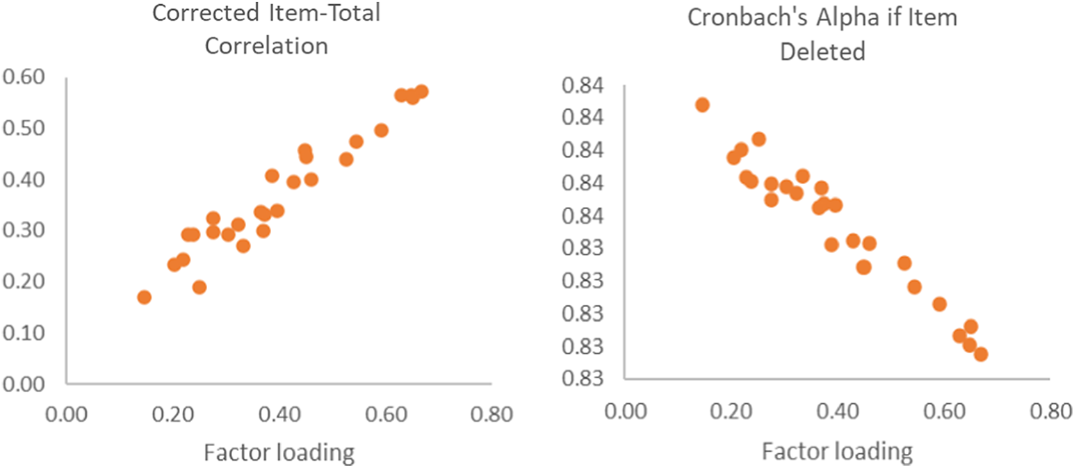
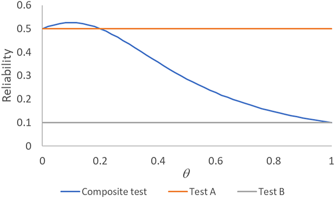


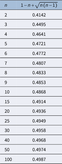

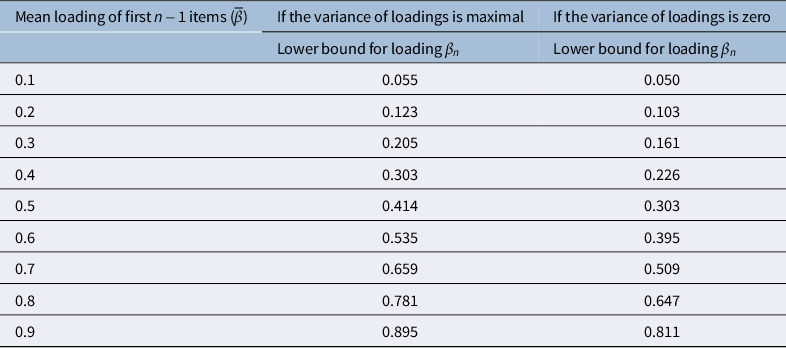
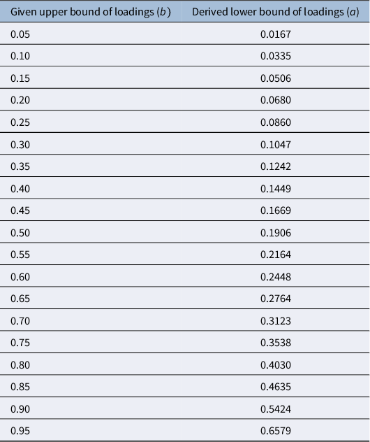


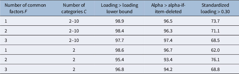
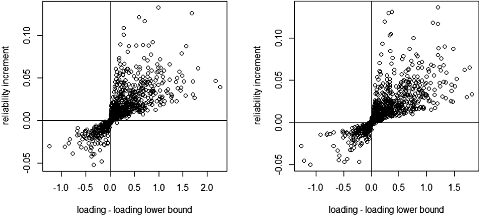
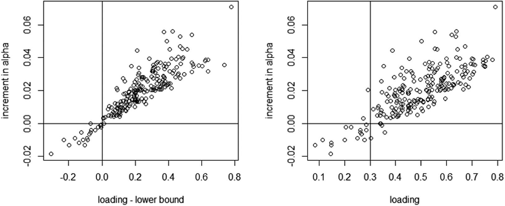


 Open access

