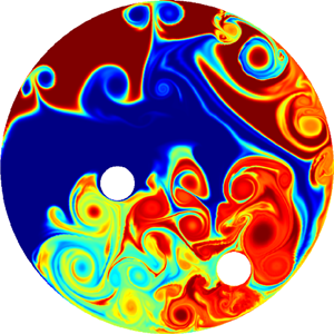
1. Introduction
The mixing of binary fluids – the process by which a heterogeneous mixture of two miscible fluids is manipulated into a homogeneous blend of uniform composition – is at the core of a great many industrial and technological applications. The food and beverage industry, as well as the consumer product industry abound with examples where multiple fluid components are mixed into a final product. Adhesives, sealants, cosmetics, inks and paints all consist of multiple ingredients that need to be mixed into their final state during a complex industrial process. Efficiency and consistency are paramount in maintaining a quality product that is cost effective to manufacture. Some of the strictest tolerances in mixing quality can be found in the pharmaceutical industry where medication has to be mixed into precise doses. But also chemical engineering processes, such as polymer production, rely on accurate mixing to facilitate the proper chemical reactions and to reduce undesirable by-products (for an overview of theoretical and practical aspects of mixing, see Paul etal. (Reference Paul, Atiemo-Obeng and Kresta2003) or Uhl (Reference Uhl2012)).
Mixing processes can be induced actively or passively. The active strategy is commonly based on a stirrer system, where paddles or rods agitate the binary mixture, induce vortical fluid structures and ultimately blend the initial ingredients. The geometry, path and speed of the stirrers have a great influence on the effectiveness and efficiency of the mixing process and are the subject of mixing optimisation. Passive systems, on the other hand, possess no moving parts, but instead rely on a complex baffle system inside an inflow-outflow device that mixes initially separated fluid components.
In this article, we will concentrate on an active stirrer system and develop a mathematical and computational framework for the formulation and solution of a constrained optimisation problem that yields favourable stirrer protocols for enhanced mixing results in binary fluid systems. Constraints stem from speed and path restrictions on the stirrers: stirrer systems are subject to mechanical and material limitations, and paddles or rods often cannot accelerate or change directions at will or too abruptly. In addition, while a significant part of industrial mixing processes involve non-Newtonian fluids, we will, for simplicity's sake, focus on Newtonian fluids. Furthermore, we will concentrate on inertial, laminar mixing. The inertial aspect of this parameter regime, described by a Reynolds number above the Stokes-flow regime, guarantees a rich and varied control space, taking advantage of advective, unsteady and diffusive processes, while the laminar aspect avoids divergences of the direct–adjoint optimisation scheme due to the existence of positive Lyapunov exponents linked to turbulent fluid motion. Despite these restrictions, a great many mixing processes fall into our chosen parameter regime.
Research in mixing has a long and remarkable history, covering theoretical aspects as well as technological applications. A large body of literature has been devoted to mixing in simplified fluid models, for example neglecting viscosity, surface tension, density differences or fluid inertia. The primary mechanism has been identified as streamline stretching (Spencer & Wiley Reference Spencer and Wiley1951) where the interface between two fluids is repeatedly distorted and redistributed into the bulk of the mixing volume. Among these simplifications, Stokes mixing, i.e. the mixing of highly viscous fluids where inertial effects can be neglected, has arguably received the most attention. This tendency has been further fuelled by the rise of micro-mixers where multiple fluid components are injected into a micro-device and extracted after the mixing process is completed (see, e.g. Orsi etal. Reference Orsi, Galletti, Brunazzi and Mauri2013; Galletti etal. Reference Galletti, Arcolini, Brunazzi and Mauri2015).
More mathematical investigations studied the breakdown in scales and the statistical properties of the observed cascade of fluid filaments. Iterated maps have often been used to determine measures that describe the pertinent scale dynamics or to design optimal mixing results in these measures (Mathew etal. Reference Mathew, Mezic, Grivopoulos, Vaidya and Petzold2007; Gubanov & Cortelezzi Reference Gubanov and Cortelezzi2010; Finn& Thiffeault Reference Finn and Thiffeault2011; Lin, Thiffeault & Doering Reference Lin, Thiffeault and Doering2011). Many of these findings can be found in Sturman, Ottino & Wiggins (Reference Sturman, Ottino and Wiggins2006). Of particular interest was the rise of chaotic mixing motion from pure advection, even for laminar flows (Aref Reference Aref1984; Ottino Reference Ottino1989; Liu Reference Liu2008).
Rather recently, the inertial, but laminar mixing regime has been explored using advances in optimisation techniques. These studies build on the definition of proper mixing measures (Mathew, Mezic & Petzold Reference Mathew, Mezic and Petzold2005; Thiffeault Reference Thiffeault2012) and break with the focus on hydrodynamic instabilities (Balogh, Aamo & Krstic Reference Balogh, Aamo and Krstic2005) to increase mixing. Using wall-mounted blowing/suction control in a channel, improved mixing could be accomplished by directly targeting a mixing measure, rather than a flow instability (Foures, Caulfield & Schmid Reference Foures, Caulfield and Schmid2014). Further studies (Marcotte & Caulfield Reference Marcotte and Caulfield2018; Vermach & Caulfield Reference Vermach and Caulfield2018) have extended this approach to higher dimensions and stratified flows.
The present article will remain in the inertial, but laminar regime and accomplish mixing of a binary fluid by embedded stirrers. These stirrers are constrained to specific paths, but can move along them in a manner that enhances mixing over a user-specified time horizon. The mixedness of the binary fluid is quantified using mix-norms (Mathew etal. Reference Mathew, Mezic, Grivopoulos, Vaidya and Petzold2007; Thiffeault Reference Thiffeault2012) for a passive scalar; an objective based on this measure is then optimised by a nonlinear, gradient-based scheme, which in turn provides the associated stirring protocol.
2. Mathematical framework
2.1. Governing equations
The focus of this study is the mixing process of a binary, miscible and Newtonian fluid by multiple circular stirrers on prescribed paths, and its optimisation by manipulating the stirring strategy within specified constraints. A two-dimensional configuration is considered. The process can be simulated by solving the fluid equations of motion, augmented by a transport equation for a passive scalar  $\theta .$ We have
 \begin{gather} {\frac{\partial}{\partial t}} {\boldsymbol{u}} + {\boldsymbol{u}} \boldsymbol{\cdot} \boldsymbol{\nabla} {\boldsymbol{u}} + \frac{1}{C_\eta}\left(\chi {\boldsymbol{u}} - \chi_k {\boldsymbol{u}}_{s,k} \right) + \boldsymbol{\nabla} p - \frac{1}{\mbox{Re}} \nabla^2 {\boldsymbol{u}} = 0, \end{gather}
 \begin{gather}\boldsymbol{\nabla} \boldsymbol{\cdot} {\boldsymbol{u}} = 0, \end{gather}
 \begin{gather}{\frac{\partial}{\partial t}} \theta + \left( (1-\chi) {\boldsymbol{u}} + \chi_k {\boldsymbol{u}}_{s,k} \right) \boldsymbol{\cdot} \boldsymbol{\nabla} \theta - \boldsymbol{\nabla} \boldsymbol{\cdot} \left( \left[ \frac{1}{Pe} (1-\chi) + \frac{\chi}{C_{\eta}} \right] \boldsymbol{\nabla} \theta \right) = 0, \end{gather}
with  ${\textbf {u}}$ as the velocity vector,
 $p$ as the pressure field and
 $\theta$ as a passive scalar (ranging from zero in one fluid to one in the other). The governing equations have been expressed in non-dimensional form using a characteristic length
 $L_0$ and velocity scale
 $u_0.$ This choice introduces the Reynolds number
 $\mbox {Re}$ and the Péclet number
 ${Pe},$ to express the kinematic viscosity and the diffusion coefficient of the mixing fluid in non-dimensional form. Furthermore, the system of (2.1c) contains terms that model the embedded stirrers via a Brinkmann penalisation approach (see Angot, Bruneau & Fabrie Reference Angot, Bruneau and Fabrie1999). The multiple solid stirrers, indexed by the subscript
 $k,$ are characterised by their velocity
 ${\textbf {u}}_{s,k},$ and are taken as circular in cross-section. The masks
 $\chi _k$ describing the embedded solid bodies equal one for points occupied by the
 $k$th stirrer and zero outside of it. The mask
 $\chi$ accounts for the overall geometry, such as the domain boundaries. The constant
 $C_\eta$ ensures the rapid relaxation of the fluid variables towards the respective values imposed by the stirrers or the geometry. The above formalism allows the efficient treatment of objects moving through a background grid on which the motion of the surrounding fluid is described. Details of this approach and its numerical implementation can be found in Eggl & Schmid (Reference Eggl and Schmid2018). The set-up shown in (2.1c) imposes no-slip velocity boundary conditions on the stirrers and no-flux Neumann conditions for the passive scalar on the solid bodies.
2.2. Measuring mixedness
In anticipation of our stated goal of enhancing mixing efficiency, we have to introduce a measure that quantifies the degree of mixedness of a particular flow state. This measure shall be based solely on the passive scalar field  $\theta$.
In general, mixing is defined as the reduction of inhomogeneities of a given indicator field (Paul etal. Reference Paul, Atiemo-Obeng and Kresta2003), which still leaves open a precise mathematical definition to be used in our case. Several norms of the passive scalar  $\theta$ that attempt to mathematically define the measure of mixedness have been proposed and used in the past (Mathew etal. Reference Mathew, Mezic and Petzold2005), among them the variance or the more complex negative-index and fractional-index Sobolev norms (Thiffeault Reference Thiffeault2012; Foures etal. Reference Foures, Caulfield and Schmid2014). As the choice of norm may influence the outcome of the optimisation, but will not affect the design of our computational optimisation platform, we will focus on the Sobolev norm of negative fractional index of the passive scalar
 $\theta .$ A measure of this general type downplays the role of small scales and instead directs mixing efforts towards larger fluid elements. It attains higher values for an unmixed field (with high levels of inhomogeneities) and decreases as the scalar field becomes more mixed. Mathematically, the mixedness measure is given as
 \begin{equation} \Vert \theta \Vert_{mix} \equiv \frac{1}{\vert V \vert} \int_{V} \Vert \boldsymbol{\nabla}^{-2/3} \theta({\textbf{x}},t) \Vert\,\text{d}V, \end{equation}
with  $V$ denoting our computational domain, and
 $\vert V \vert$ representing its size (volume or area). In the above definition, we have assumed, without loss of generality, a zero mean of the passive scalar field
 $\theta .$ Throughout this paper we will be optimising with respect to this quantity, but we stress again that other norms can be employed without conceptual changes in the optimisation procedures. For our study, we select the mix-norm with an exponent
 $k$ of
 $-2/3$, a value between the common choice
 $k=-1$ (see Lin etal. Reference Lin, Thiffeault and Doering2011; Foures etal. Reference Foures, Caulfield and Schmid2014; Marcotte & Caulfield Reference Marcotte and Caulfield2018) and the choice of
 $k=-1/2$ proposed by Mathew etal. (Reference Mathew, Mezic and Petzold2005) based on advection-based mixing. In general, the exponent governs the relative emphasis of larger over smaller scales in the definition of mixedness, as can be seen from a Fourier transform of the integrand in the expression above. While the choice
 $k=-1$ is equivalent to an integral over the considered domain, the fractional exponents
 $k=-1/2$ and
 $k=-2/3$ produce a more complex coupling of local phenomena throughout the domain. Varying the exponent
 $k$ will have quantitative consequences; qualitatively, however, the mixing strategies and their interplay (shown below) will remain the same. A detailed parameter study of the exponent is beyond the scope and interest of the current study.
2.3. Mixing protocol
As a first attempt at optimising the mixing of a binary fluid, we will concentrate on a stationary circular vessel with two stirrers on circular paths of distinct radii (see figure 1 for a sketch of this configuration). For this investigation, we choose a zero rotation about the stirrers’ centre, i.e.  $\Omega _k = 0.$ Furthermore, the radii have been selected to avoid collision of the stirrers on their respective paths. The stirrers have a circular cross-section, and their velocities along their trajectories are undetermined and subject to optimisation and constraints. The circular path is conveniently defined in polar coordinates, while we formulate the remaining equations in Cartesian coordinates, and we thus introduce the vector-valued function
 $\boldsymbol {l}$, which transforms between the two coordinate systems according to
 $(l_1(\phi ),l_2(\phi )) = (-\sin (\phi ),\cos (\phi ))$ with
 $\phi$ as the angle traversed along the path of the circle. The parameterisation of the velocity of the
 $k$th stirrer thus becomes
 \begin{equation} \boldsymbol{u}_{s,k} =\omega_{k}(t)\boldsymbol{r}_k(\boldsymbol{x})\boldsymbol{l}(\varphi_k(t)), \end{equation}
where  $\varphi$ is the sum of the angles travelled along the path, i.e.
 \begin{equation} \varphi_k(t) = \int_0^t\omega_{k}({ \tau})\,\text{d}{ \tau}. \end{equation}
Following the notation of the governing equations, we define  $\omega _k(t)$ as the rotational speed of the
 $k$th solid about the centre of the vessel and
 $\boldsymbol{r}_k$ denotes the distance from the same centre.
Set-up of mixing problem. A circular domain of radius  $R$ encloses two stirrers of circular cross-section (given by radii
 $a_{1,2}$) on concentric circular paths of fixed radii
 $r_{1,2}.$ The stirring strategy is determined by the time-dependent circular velocities
 $\omega _{1,2}(t),$ together with the rotation rate
 $\Omega _{1,2}$ about each cylinder's axis. For simplicity, we choose
 $\Omega _{1,2}=0$ in this study. Initially, one fluid component occupies the lower half of the vessel, while the other fluid component resides in the upper half.

2.4. Constrained optimisation
We can then state the optimisation problems as finding a time-dependent velocity protocol  $\omega _k(t)$ for each of the two stirrers such that the mix-norm of the passive scalar is minimised over a prescribed time horizon. This minimum has to be achieved while satisfying the governing equations and respecting constraints and bounds on the stirrer velocities. Mathematically we have
 \begin{gather} \min \left\{ \int_0^{T} \Vert \theta \Vert_{mix}\,\textrm{d} t \right\} \end{gather}
 \begin{gather} \textrm{subject to equations (2.1)} \end{gather}
 \begin{gather}\hbox{and} \quad \int_0^{T} \sum_k \Vert \boldsymbol{u}_{s,k} \Vert^2 \,\textrm{d} t \leq E_0 \end{gather}
 \begin{gather}\hbox{and} \quad \boldsymbol{u}_{s,{lower}} \leq \boldsymbol{u}_{s,k} \leq \boldsymbol{u}_{s,{upper}}\quad k=1,2, \end{gather}
 \begin{gather}\hbox{and} \quad \boldsymbol{a}_{s,{lower}} \leq \boldsymbol{a}_{s,k} \leq \boldsymbol{a}_{s,{upper}}\quad k=1,2. \end{gather}
The constraints on the stirrer strategy are threefold: the first constraint limits the  $L_2$-norm of
 $\boldsymbol {u}_s$, i.e. the kinetic energy of the stirrers’ motion along their paths, expended over the time horizon
 $T$ to a maximum value of
 $E_0;$ the second and third impose upper and lower bounds directly on the stirrers’ velocities and accelerations, respectively. All restrictions could conceivably stem from mechanical limitations of the mixing apparatus. In our study, we will consider the constraints successively in order to determine the influence they impose on the optimisation results.
3. Computational framework
The implementation of the above optimisation problem requires the discretisation of the governing equations and the reformulation of the constrained problem (2.5) in terms of an unconstrained one.
3.1. Numerical scheme for the governing equations
Starting point for the numerical treatment of mixing enhancement is the open-source FLUSI software (Engels etal. Reference Engels, Kolomenskiy, Schneider and Sesterhenn2015), in which the governing equations are discretised on a Cartesian, double-periodic domain for the two-dimensional case. This formulation allows the application of Fourier-spectral techniques to represent the spatial derivatives. The outer perimeter of the mixing vessel (with radius  $R$) and the two stirrers on their respective circular paths (with radius
 $r_1$ and
 $r_2$) are described by a Brinkman penalisation technique as shown in (2.1c). The original software has been augmented by the passive scalar field and embedded into a gradient-based optimisation formalism.
The Fourier-spectral discretisation allows the replacement of spatial derivatives with a multiplication by components of a wavenumber vector 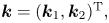 $\boldsymbol{k} = (\boldsymbol{k}_1,\boldsymbol{k}_2)^{\textrm {T}},$ with the indices
 ${}_{1,2}$ indicating the two coordinate directions. Mathematically, we introduce this replacement as
 $\partial /\partial x_j \to {\textsf {A}}_j,$ with
 ${\textsf {A}}_j = \hbox {diag}\{ \textrm {i}\boldsymbol{k}_j \}.$ The semi-discretised set of equations then reads
 \begin{gather} {\frac{\textrm{d}}{\textrm{d} t}} {\boldsymbol{u}}_i + {\boldsymbol{u}}_j \circ \left[ {\textsf{A}}_j {\boldsymbol{u}}_i \right] + \frac{1}{C_\eta}\left(\chi \circ {\boldsymbol{u}}_i - \chi_k \circ {{\boldsymbol{u}}_{s,k}}_i\right) + {\textsf{A}}_i p - \frac{1}{Re} {\textsf{A}}_j {\textsf{A}}_j {\boldsymbol{u}}_i = 0, \end{gather}
 \begin{gather}{\textsf{A}}_j {\boldsymbol{u}}_j = 0, \end{gather}
 \begin{gather}{\frac{\textrm{d}}{\textrm{d} t}} \theta + \left( (\textbf{1} - \chi) \circ {\boldsymbol{u}}_j + \chi_k \circ {{\boldsymbol{u}}_{s,k}}_j \right) \circ \left[ {\textsf{A}}_j \theta \right] - {\textsf{A}}_j \left[ \frac{1}{Pe} \left( \textbf{1} - \chi \right) + \kappa \chi \right] \circ {\textsf{A}}_j \theta = 0, \end{gather}
where we introduced the Hadamard (element-wise) product  $\circ$ (see Horn & Johnson Reference Horn and Johnson2012) and assumed implicit (Einstein) summation over identical indices.
Particular care has to be exercised when evaluating the nonlinear terms, as aliasing errors can lead to inaccuracies and numerical instabilities. A low-pass Hou–Li filter (Hou & Li Reference Hou and Li2007) has been applied to avoid scattering of unresolved, small scales onto resolved, large scales. In addition, P3DFFT (Pekurovsky Reference Pekurovsky2012), a highly efficient, parallel Fourier-transform library, is used to ensure scaling on parallel computer architectures.
Finally, the representation of solid bodies on an underlying Cartesian grid calls for a transfer of geometric information onto the background mesh. This transfer is accomplished by mollified delta-functions, smoothing the otherwise discontinuous mask onto the grid and thus avoiding numerical inaccuracies and instabilities (Kolomenskiy & Schneider Reference Kolomenskiy and Schneider2009).
3.2. From constrained to unconstrained optimisation
A common reformulation of the constrained optimisation problem (2.5) as an unconstrained problem introduces Lagrange multipliers (or adjoint variables) for the dependent variables of (2.1c): the adjoint velocity will enforce the momentum equation, the adjoint pressure the divergence condition and the adjoint passive scalar the transport equation for  $\theta .$ The augmented Lagrangian – consisting of the cost functional and the scalar product of the adjoint variables and the governing equations – then needs to be minimised. A system of equations, referred to as the Karush–Kuhn–Tucker (KKT) system, can then be derived by setting to zero the first variation of the augmented Lagrangian with respect to direct (original) and adjoint variables. The first variation with respect to the adjoint variables recovers the original set of governing equations. The first variation with respect to theoriginal variables produces, after considerable algebra, a set of equations governing the adjoint variables. The first variation with respect to the control variables (in our case, the velocity strategies
 $\omega _{1,2}(t)$) will furnish the gradients of the cost functional with respect to
 $\omega _{1,2}(t)$ which will be used to enhance the mixedness of our fluid system via improved stirring strategies.
3.3. Adjoint equations
Denoting the adjoint variables (velocity, pressure, passive scalar) by  ${\textbf {u}}^{\dagger }$,
 $p^{\dagger }$ and
 $\theta ^{\dagger},$ the governing equations for their evolution, in semi-discretised form, read
 \begin{align} & {\frac{\textrm{d}}{\textrm{d} t}} {\boldsymbol{u}}^{\dagger}_i - \Pi^{\dagger}_k \circ [{\textsf{A}}_i {\boldsymbol{u}}_k ] - {\textsf{A}}_j^H [{\boldsymbol{u}}_j \circ \Pi^{\dagger}_i] - \frac{\chi}{C_{\eta}} \circ \Pi^{\dagger}_i + \frac{1}{\mbox{Re}}{\textsf{A}}_j^H {\textsf{A}}_j^H {\boldsymbol{u}}_i^{\dagger} \nonumber\\ &\quad -(\textbf{1}-\chi) \circ \theta^{\dagger} \circ[ {\textsf{A}}_i \theta] = 0, \end{align}
 \begin{align} & {\textsf{A}}_j^H \Pi_j^{\dagger} = 0, \end{align}
 \begin{align} & {\frac{\textrm{d}}{\textrm{d} t}} \theta^{\dagger} - {\textsf{A}}_j^H [(\textbf{1}-\chi) \circ {\boldsymbol{u}}_j \circ \theta^{\dagger}] + {\textsf{A}}_i^H \left(\left[\frac{1}{Pe}(\textbf{1}-\chi) + \kappa\chi\right] \circ {\textsf{A}}_i^H \theta^{\dagger}\right) \nonumber\\ &\quad -{\textsf{A}}_j^H [ \chi_i \circ ({\boldsymbol{u}}_{s,i})_j\ \circ \theta^{\dagger}] = 0, \end{align}
with terminal conditions
 \begin{equation} \boldsymbol{u}^{\dagger}(\boldsymbol{x},T) = 0,\quad \theta^{\dagger}(\boldsymbol{x},T) = \frac{2}{V_\Omega}\left(\mathsf{A}_i^{-2/3}\right)^H\left(\mathsf{A}_i^{-2/3}\theta(\boldsymbol{x},T)\right). \end{equation}
It is important to note that the above adjoint equations are linear in the adjoint variables, but are dependent on the direct variables  ${\textbf {u}}_i.$ Moreover, it should become apparent that the adjoint equations have to be solved backwards in time, from
 $t=T$ to
 $t=0.$
The optimality conditions, stemming from the first variation with respect to the control variables, result in the adjoint rotational velocity along the circular paths given by
 \begin{equation} \omega_{k}^{\dagger} = r_i\left[l_j(\varphi(t)) +\frac{\omega_{k}}{\dot{\omega_{k}}} \frac{\partial l_j}{\partial \varphi}\right]\chi_i^H\left(\frac{\Pi^{\dagger}_j}{C_\eta}- (\theta^{\dagger}\circ[\mathsf{A}_j\theta])\right), \end{equation}
where  $\Pi ^{\dagger }_i = {\textbf {u}}^{\dagger }_i + {\textsf {A}}^{H}_i p^{\dagger }$. This value provides the gradient information in our iterative optimisation scheme and, together with a line-search routine, updates the current stirring protocol to a more effective one. The optimisation terminates when no more progress can be made, and the magnitude of the cost functional gradient drops below a prescribed threshold.
3.4. Implementing additional constraints
Additional constraints that need to be enforced are incorporated into the gradient-based optimisation routine. This can be accomplished in two ways: by adding penalty terms in the cost functional, or by using projections and thresholding. We opt for the latter choice: the gradient – computed from the adjoint equations and the optimality condition, without imposed constraints – is projected and properly curtailed to comply with energy constraints and velocity and acceleration bounds. While mathematically equivalent, the projection technique is easier to implement and presents more flexibility in treating inequality constraints. Details of the numerical implementation of this procedure can be found in Eggl & Schmid (Reference Eggl and Schmid2018).
3.5. Summary of optimisation procedure
The full optimisation scheme then proceeds along the following lines. Starting with an initial guess of the stirring protocols  $\omega _{1,2}(t),$ we solve the governing equations (2.1c) forward in time over a chosen time horizon
 $[0, T].$ In a second step, the adjoint set of (3.2c) are solved, starting with the proper terminal condition, backwards in time from
 $t=T$ to
 $t=0.$ The adjoint variables are then used to evaluate the optimality condition and retrieve the gradient of the cost functional with respect to
 $\omega _{1,2}.$ This gradient is then furnished to a standard optimisation routine (such as steepest descent or conjugate gradients) which, together with a line-search routine, produces a new and improved stirring protocol. In this last step, all constraints imposed on the stirring functions will be imposed by the aforementioned projections and thresholding. After this step, the next iteration is started. The optimisation terminates when no further progress can be made, within the constraints imposed on the system.
It is worth mentioning that additional complications arise from the fact that the governing equations (2.1c) are nonlinear and, as a consequence, the adjoint equations (3.2c), while linear in the adjoint variables, depend on the direct variables  $\textbf {u}, \theta .$ This dependency requires the storage of direct fields during the simulation of (2.1c) and their injection into (3.2c), in reverse order, during the integration of the adjoint system. For efficiency reasons, this exchange between direct and adjoint simulations is handled by checkpointing, where we trade excessive storage requirements for an increased simulation time. The revolve library (Griewank & Walther Reference Griewank and Walther2000) accomplishes this task in an optimal manner.
4. Test cases and results
We follow the set-up shown in figure 1 with two circular cylinders of radius  $a_{1,2}= 0.5,$ moving on two concentric circular paths of radius
 $r_1 = 3.5$ and
 $r_2 = 1.5$ and embedded in a circular (stationary) vessel of radius
 $R = 5.$ The Reynolds number and Péclet number are chosen as
 $Re = Pe = 1000.$ The numerical resolution of our simulations is
 $512 \times 512$ equispaced grid points in the two Cartesian coordinate directions, and convergence studies have been performed to ensure grid-independent solutions.
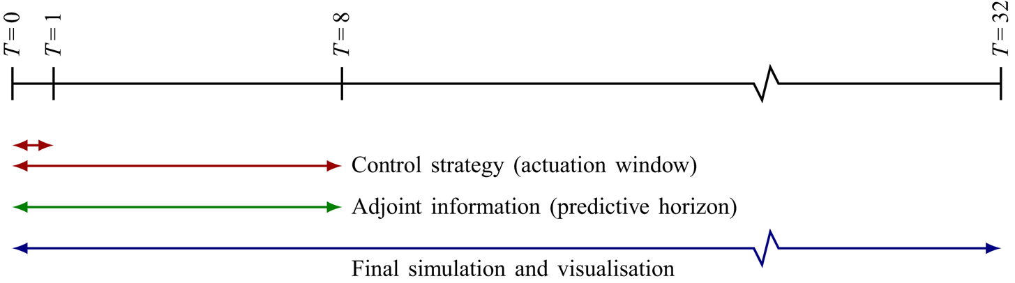
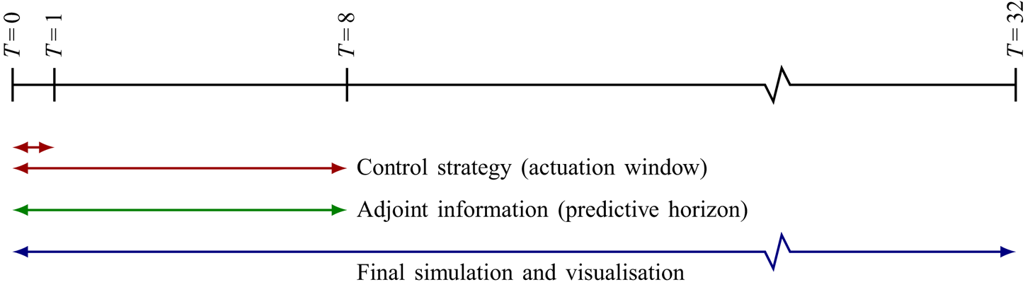
A further parameter in the optimisation concerns the time horizons over which (i) the control strategy is applied, and (ii) over which gradient information is gathered. The former time interval determines the window given to the stirrers to be active mixers; after this window is passed, the motion of the stirrers will stop, and only the remaining inertia of the fluid and diffusion will contribute to further mixing. The latter time interval determines the amount of information extracted from the evolution process that is used to compute an enhanced stirring protocol (applied over the former time window). The control horizon may be chosen shorter than the information (predictive) horizon: in this case, a time-compressed strategy will be employed that accounts for, and optimises over, a more expansive time window. In our case, we will juxtapose a short-term strategy with  $T_{control}=1$ and a longer-time strategy with
 $T_{control}=8$ and assess the optimised strategies in either case. Both protocols, however, have access to information over a temporal interval of
 $T_{info} = 8.$ Finally, the simulations have been continued over
 $T_{sim}=32$ units to track the further development of the instigated mixing processes; rest inertia and diffusion will remain the only mechanisms during this stage. A summary of our choice of parameters is sketched in figure 2.
Sketch of time horizons for the optimisation problem. A control strategy (red) is applied over two control horizons,  $T_{control}=1$ (for short-time control) and
 $T_{control}=8$ (for long-time control). The gradient information about the flow development (green), encoded in the adjoint variables, is gathered over a predictive horizon of
 $T_{info}=8.$ The final simulation, based on the optimised strategy, is performed over
 $T_{sim}=32$ non-dimensional time units (blue).
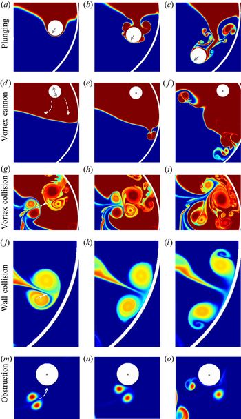
Before proceeding to the various optimisation studies, it is instructive to reflect upon possible mixing mechanisms given the set-up in figure 1. The most obvious strategy for mixing a binary fluid consists of a plunging motion, where the cylinders push through the initial interface, distort it and drag fluid one into regions occupied by fluid two, and vice versa (figure 3a–c). This type of strategy is nearly exclusively implemented in industrial mixers. Despite its omnipresence in applications, alternative strategies are often equally or more effective, foremost among them vortex shedding due to unsteady and abrupt motion of the stirrers, affably denoted as the vortex cannon strategy (figure 3d–f). In this case, the stirrer generates a sequence of start up and stopping vortices by rapid oscillations or abrupt directional changes along the circular paths. The shed vortices then act as effective autonomous mixers that, once they reach the initial or distorted interface, further deform the passive scalar field and locally (and globally) reduce the mix-norm. In this manner, a single stirrer can clone ‘fluid stirrers’ (shed vortices) and thus multiply its mixing effectiveness. In a further possible strategy, vortices can be generated in the fluid that collide with each other and thus generate filaments, which are then subjected to more rapid diffusion and homogenisation (figure 3g–i). Of course, this vortex collision strategy is strongly dependent on the initial condition of the passive scalar – and for this reason, less transferable to a general, realistic mixing strategy – nonetheless, within our computational framework, it is a viable and pervasive strategy utilised by our direct–adjoint algorithm. Afar more transferable mixing strategy is the collision of vortical structures with the outer wall (figure 3j–l) (wall collision) whereby a large fluid element is broken up into smaller elements which further interact with other vortices and are subject to increased diffusion due to the breakdown in scales. Finally, the embedded physical stirrers can themselves interplay with the vortical structures they generate, acting as obstructions in the path of vortices (figure 3m–o). A collision between a stirrer and a vortex will split the vortex and yield smaller scales, hence contributing to a decrease in the mix-norm. This final strategy will continue to cause a moderate breakdown in scales, even after the control window has closed and no more stirring motion is allowed.
Various mixing strategies, from snapshots of the simulations. (a–c) Plunging of the stirrer through the interface, (d–f) casting of start–stop vortices towards the interface (vortex cannon), (g–i) collision of vortices, (j–l) collision with the vessel wall and (m–o) breakup of vortical structures by stationary stirrers (obstruction). Grey arrows in the above figures present the motion of the stirrers based on the optimal strategy; the white dashed arrows in each panel indicate the key processes responsible for efficient mixing and have been added to guide the reader.
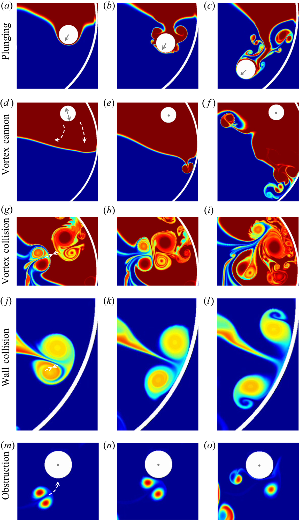
Given these five fundamental strategies, illustrated in figure 3 with samples from our simulations, the direct–adjoint looping algorithm will select from and combine these options into a coherent strategy, given the chosen parameters and user-specified constraints.
4.1. Overview of test cases
We will consider six cases, grouped into three examples. Each example consists of a short-time strategy with a rather limited control horizon of  $T_{control}=1$ and a long-time strategy with a more generous horizon of
 $T_{control}=8.$ These two
 $T_{control}$-settings will impose noticeable constraints on the choice of strategies, the interplay of dynamic processes and the feasibility of the final protocol. The three examples further distinguish themselves by the number of external constraints: starting with pure energy constraints, via energy and velocity constraints, to energy, velocity and acceleration constraints.
Convergence of the iterative scheme is principally governed by constraints imposed on the optimisation problem. First, the nonlinear nature of the governing equations precludes a guarantee to converge towards a global minimum; only a local minimum can be expected. More importantly, additional constraints on the stirrers, such as energy, velocity or acceleration bounds, can convert a semi-norm to a full-norm optimisation problem. Semi-norm optimisation problems (Foures, Caulfield & Schmid Reference Foures, Caulfield and Schmid2012; Blumenthal etal. Reference Blumenthal, Tangirala, Sujith and Polifke2017) are ‘open ended’ in the sense that the stirrer velocities increase without bounds, while the mixing measure steadily improves. In this case, the iterative optimisation scheme terminates when the adjoint variables, due to excessive direct velocities, no longer furnish useful gradient information for further improvement. In other words, the optimisation comes to an end when the signal-to-noise ratio for the gradient information drops to a value near unity, even before the cost-functional gradient attains a small value. In the full-norm case, convergence is achieved when the cost-functional gradient falls below a small, user-specified threshold, indicating that a local minimum has been reached. Iterations are halted when either the cost-functional gradient falls below a small threshold or the signal-to-noise ratio of the adjoint gradient information reaches unity – whichever scenario comes first.
Since mixing enhancement based on complex stirring strategies is a highly dynamic process – based on a rapid sequence of abundant vortical features – a set of static snapshots cannot do justice to the intricacies of an optimised mixing protocol. For this reason, we urge the reader to turn to the animations in the supplemental material available at https://doi.org/10.1017/jfm.2020.448.
4.2. Cases 1 and 2: optimisation under energy constraints
The first two cases follow a common procedure whereby the cost functional (mix-norm of the passive scalar) of the constrained optimisation is minimised, subject to a penalisation of the control energy that accomplishes this minimum. As a consequence, the energy expended by the stirrers is bounded to a user-specified value. This value has been chosen as the maximum energy level that, over the selected time horizon, still maintains a signal-to-noise ratio above one for the adjoint information. In this manner, we allow a maximum of energy injected into the stirring, while maintaining control over the manner in which it is expended by the stirrers. For all control strategies shown below, this upper energy bound is always reached.
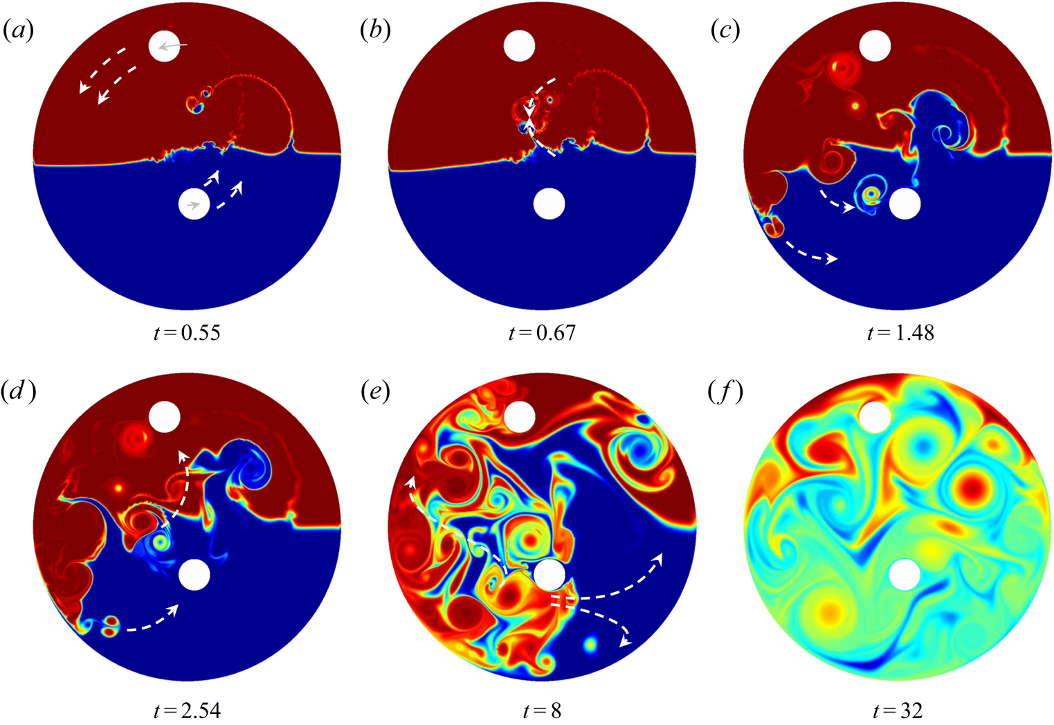
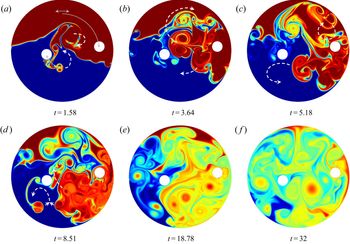
Figure 4 displays the results of our optimisation, visualised by iso-contours of the passive scalar  $\theta$ at selected time instances. The control horizon is
 $T_{control}=1.$ We observe that the optimisation does not utilise the ‘plunging’ option, as the stirrers remain nearly at their initial position. Instead, the entire energy available to the stirrers is used up in a rapid start-and-stop motion which initially causes multiple small-scale shed vortices that distort the plane interface, collide into each other and the stirrers, and merge into larger-scale vortex structures which eventually achieve good mixing. It is important to stress that for the calculation of this short-time mixing strategy, information about the full dynamics up to
 $T_{info}=8$ has been incorporated into the optimisation. In other words, the consequences of the limited stirring protocol up to
 $T_{info}=8$ are known to the optimisation, and adjustments to the control strategy can be made that affect the vortex dynamics beyond its active control window. The evolution of the passive scalar between
 $T_{info}=8$ and
 $T_{sim}=32,$ however, is neither designed nor recognised by the optimisation algorithm; it simply plays out according to the action taken during the control and optimisation windows. We include this further evolution to underline our choice of the mix-norm as the mixedness measure, whose optimisation produces the small scales that are subsequently diffused during this ‘cool-off’ window.
Mixing optimisation based on only energy constraints for the stirrers. The time horizon for applying control is  $T_{control}=1.$ Shown are iso-contours of the passive scalar at selected instances. The optimisation algorithm includes information over a time window of
 $T_{info}=8.$ Grey arrows in (a) present the motion of the stirrers based on the optimal strategy; the white dashed arrows in each panel indicate the key processes responsible for efficient mixing and have been added to guide the reader. A more detailed impression of the full mixing process can be gained from the supplementary movies.

We conclude that the absence of any plunging option points at the suboptimality of this particular strategy in achieving an enhanced mixing process. It is thus not pursued as a viable option by the direct–adjoint optimisation technique. In the interpretation of these results, it may be tempting to conclude that a different initial placement of the cylinders – closer to the initial interface – would have resulted in strategies that included plunging. However, a simulation of the same case (not shown), with the two cylinders starting immersed in the initial interface, came to the same conclusion: while, by design, there is a small amount of plunging in this case, the vast majority of the mix-norm reduction has been accomplished by the shedding of start-and-stop vortices by a vigorous oscillatory motion of either cylinder and a subsequent collision of the generated vortices. The utilisation of the stirrers’ energy to shed small ‘vortical stirrers’ is a better strategy than the distortion of the interface by simply moving through it with the stirrers.
The later part of the stirring strategy includes vortex collisions (see figure 4b), obstruction by the stirrers (see figure 4c,d) and collision with the outer wall (see figure 4e) to yield a well-mixed state at the end of the simulation horizon (figure 4f).
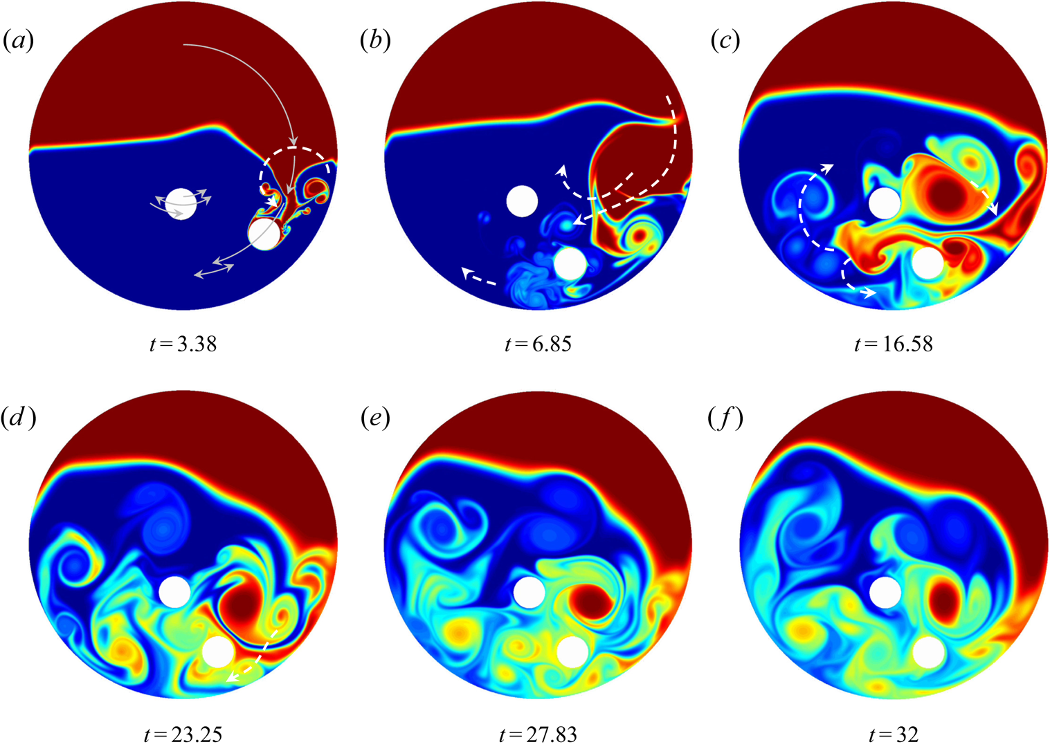
Increasing the control horizon from  $T_{control}=1$ to
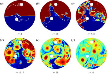
 $T_{control}=8$, which can be seen in figure 5, leads to similar conclusions, even though the stirring action by the cylinders is less abrupt and less jarring. Still, the bulk of the mixing action is achieved by shedding start-and-stop vortices which collide with themselves, secondary vortices and the wall to produce a mixed state in theend. Again, the absence of plunging is noteworthy. This is even more remarkable, as the increased control time horizon would certainly allow the stirrers to approach and reach the interface; yet, they remain close to their initial position.
Same as figure 4, but with an extended control window of  $T_{control}=8.$

In both cases, the strategy found by the direct–adjoint optimisation technique will yield increasingly larger velocities, as long as the integrated energy is constant. Eventually, the energy expenditure becomes more and more localised in time, with the stirrers barely moving. This optimisation route is a logical consequence of our current set-up. It is closely connected to the semi-norm problem (see Foures etal. Reference Foures, Caulfield and Schmid2012; Blumenthal etal. Reference Blumenthal, Tangirala, Sujith and Polifke2017): the mix-norm only contains the passive scalar  $\theta$, but does not account for the other dynamic variable, the velocities, in the optimisation. The energy of the stirrers is not sufficient to arrive at realistic stirring protocols that could be implemented in an experimental or industrial setting. To ensure applicability of our stirrer strategies to real-life settings, additional constraints are required.
4.3. Cases 3 and 4: optimisation under energy and velocity constraints
Following the findings of the previous section, in the next examples we limit the velocity of the stirrers to avoid excessive values of  $\textbf {u}_{s,i}.$ This capping of the velocity is implemented by a projection of the raw cost-functional gradient onto control strategies that satisfy the given constraints (for details of this projection technique see Foures etal. Reference Foures, Caulfield and Schmid2014). The limit on the stirrer velocities counteracts the previous temporal localisation of the stirring protocol. As a consequence, an extended and smoother movement of the stirrers is expected.
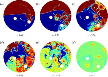
For the shorter control horizon  $T_{control}=1,$figure 6 shows the outcome of our optimisation. The top stirrer starts by an oscillatory motion, exploiting again the ‘vortex cannon’ strategy. Both stirrers then move closer to the (already distorted) interface. But rather than plunging through it, they abruptly stop short of it and let the overtaking stop vortices carry out the distortion of the interface and the subsequent mixing. The remaining mixing process is characterised by vortex collision (see figure 6a,d), collision with the wall (see figure 6c) and stirrer obstruction (see figure 6c,d).
Mixing optimisation based on energy and velocity constraints for the stirrers. The time horizon for applying control is  $T_{control}=1.$ Shown are iso-contours of the passive scalar at selected instances. The optimisation algorithm includes information over a time window of
 $T_{info}=8.$ Greyarrows in (a) present the motion of the stirrers based on the optimal strategy; the white dashed arrows in each panel indicate the key processes responsible for efficient mixing and have been added to guide the reader. A more detailed impression of the full mixing process can be gained from the supplementary movies.

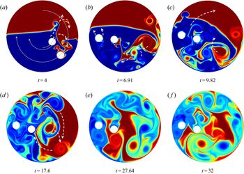
Extending the horizon  $T_{control}$ results in a change of strategy (see figure 7). The top stirrer now plunges through the interface – but not before stopping and starting on its circular path towards it. This uneven motion creates more vortical structures in the stirrer's wake that add to the sole plunging action of the stirrer itself. The result is a far more distorted interface (and consequently a lower mix-norm) than would be generated by a simple traversal. At the end of the motion, a back-and-forth motion is performed to generate additional shed vortices that further interact with the interface and other vorticalelements. The second stirrer does not follow the strategy of the first. It rather engages in an oscillatory motion similar to case 2 above. As before, obstruction by the cylinders (see figure 7b,d) and vortex and wall collisions (see figure 7c,d) contribute to the continued mixing.
Same as figure 6, but with an extended control window of  $T_{control}=8.$

In both cases, a gentler stirring strategy is observed. However, while we explicitly avoid highly localised action of the stirrers with excessive velocities, we now tend towards favouring strategies with excessive acceleration. This should not come as a surprise as the strength of shed vortices from the stirrers’ unsteady motion is proportional to their acceleration. Our imposed constraints do account for energy and velocities, but not velocity gradients, of the stirrers. As a consequence, we can seed our binary mixture with vortical elements of nearly unlimited strength. To limit the velocity of the fluid, we have to limit the acceleration of the stirrers. Again, additional constraints are necessary.
4.4. Cases 5 and 6: optimisation under energy, velocity and acceleration constraints
Based on the observations and conclusions from our previous cases, we augment our optimisation scheme by terms accounting for the stirrers’ acceleration. Within our computational framework, additional projections are used to enforce these acceleration constraints. While the energy bound is chosen to maintain a viable adjoint signal and the velocity bounds are selected to match this energy bound via their integral over the time horizon, the choice of acceleration bounds is less obvious. For this reason, we progressively reduce the upper acceleration bounds until we first experience a marked drop in total variation of the stirrer velocities, thus eliminating an undesired highly oscillatory mixing strategy.
For the short-term control with  $T_{control}=1$ (see figure 8), the optimal strategy now includes a plunging of the first cylinder through the interface, while the second cylinder continues in a straight manner towards the interface but stops short of it. The resulting vortices from this motion are responsible for the bulk of the mixing. Initiated by this motion, complex vortex collisions (see figure 8c), stirrer obstruction (see figure 8c,d) and wall interactions (see figure 8d) contribute greatly to the breakdown of scales, the generation of filaments (see figure 8e) and the eventual mixing of the binary fluid (see figure 8f).
Mixing optimisation based on energy, velocity and acceleration constraints for the stirrers. The time horizon for applying control is  $T_{control}=1.$ Shown are iso-contours of the passive scalar at selected instances. The optimisation algorithm includes information over a time window of
 $T_{info}=8.$ Grey arrows in (a) present the motion of the stirrers based on the optimal strategy; the white dashed arrows in each panel indicate the key processes responsible for efficient mixing and have been added to guide the reader. A more detailed impression of the full mixing process can be gained from the supplementary movies.

A longer control horizon of  $T_{control}=8$ (see figure 9) yields a more varied stirring protocol. The first cylinder plunges through the interface, but not without halting to shed additional vortices close to the interface, before stopping on the opposite side of the vessel and shedding two stop vortices that further distort the interface on the left. The second cylinder approaches the interface, ejects a stop vortex before reversing and stopping short of the interface with another stop vortex. Compared to the short-term strategy, less homogeneity (larger mix-norm) is observed. This reduced homogeneity can be attributed to the restricted velocity range.
Same as figure 8, but with an extended control window of  $T_{\textit{control}}=8.$

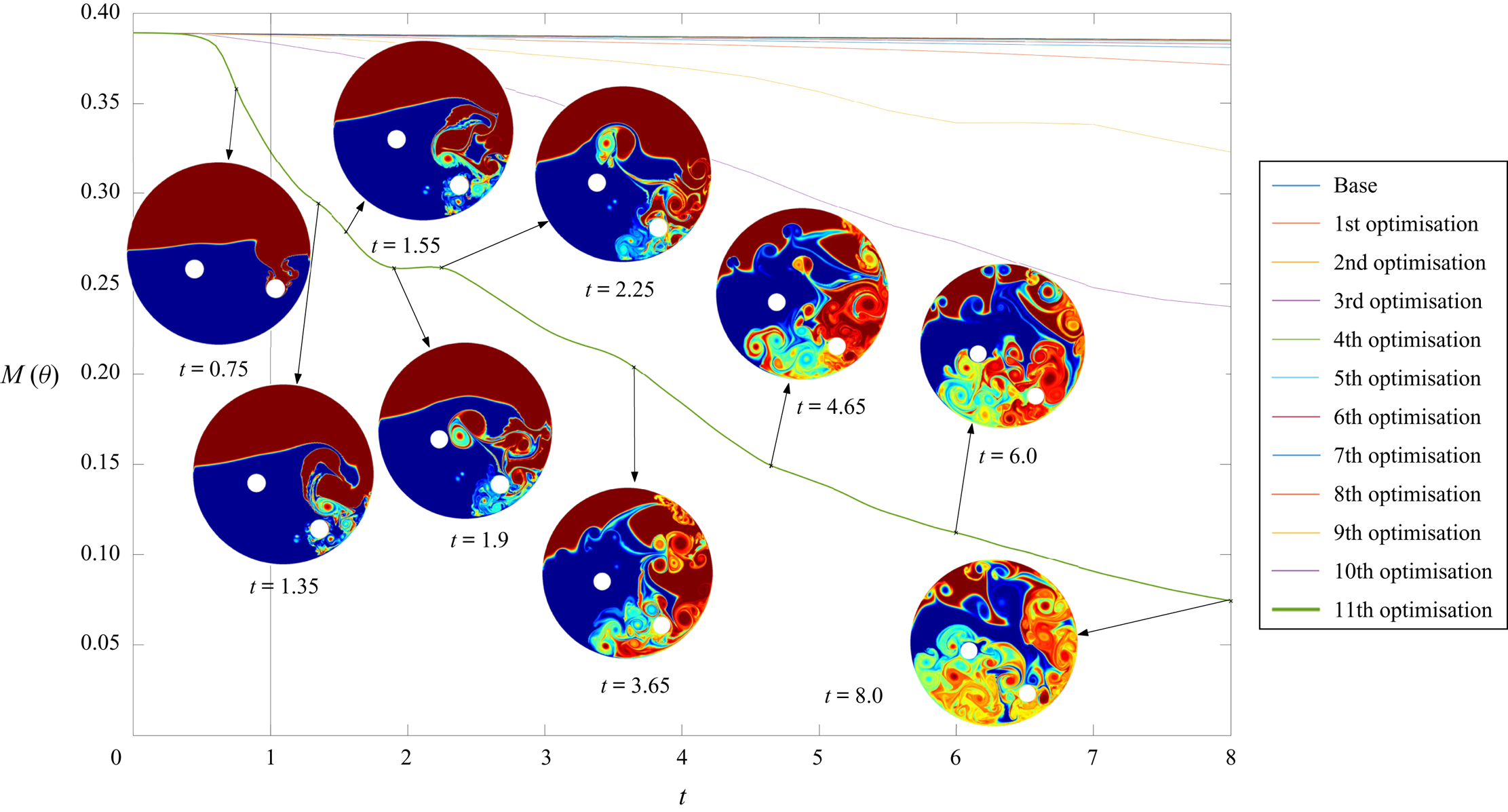
Figure 10 illustrates the optimisation procedure and the final mixing strategy by displaying the mix-norm versus time for the various iterations of the direct–adjoint looping technique. The first few iterations accomplish only a modest decrease in mix-norm. However, after a promising strategy has been identified (given by a distortion of the interface by shed vortices), the gradient information furnished by the adjoint equation causes the optimisation to further pursue this direction and fine-tune the strategy. Consequently, the mix-norm decreases monotonically and more precipitously, until it converges to a final stirring protocol. For this strategy, figure 10 superimposes snapshots of the passive scalar field at representative instants in time along the mix-norm curve. While a drop in mix-norm can be associated with the development of small scales induced by the vortex dynamics (see, for example,  $t=0.75$), we also observe occasional plateaus (for example, between
 $t=1.9$ and
 $t=2.25$) where the passive scalar field simply rearranges itself via advection rather than exhibits a further breakdown in scale. The final value of the mix-norm at
 $t=8$ is significantly lower than intermediate values, indicating a substantially enhanced mixing process, evident in the accompanying passive scalar snapshot.
Mixing optimisation based on energy, velocity and acceleration constraints for the stirrers. The time horizon for applying control is  $T_{\textit{control}}=1.$ Shown is the evolution of the mix-norm over time, for the various iterations of the direct–adjoint looping scheme. For the final result, snapshots of the passive scalar field are superimposed to visualise the enhanced mixing process.

5. Summary, conclusions and remaining challenges
A direct–adjoint optimisation methodology has been applied to the problem of mixing of binary fluids. A circular configuration with two embedded stirrers on circular paths has been chosen, and the velocities of these two stirrers over a user-specified time interval have been determined in an attempt to enhance the homogeneity of the binary mixture. The gradient-based optimisation is effective in finding stirring protocols that yield enhanced mixing results, but convergence towards an optimum crucially relies on imposing proper constraints on the iterative algorithm. Since the mixing efficiency is based on only one dynamic variable, the passive scalar  $\theta ,$ but disregards the velocity fields, additional external constraints have to be imposed to properly define a feasibleoptimum. By restricting the stirrers’ maximum acceleration in addition to energy and velocity bounds, we arrive at a properly stated optimisation problem and a convergent direct–adjoint algorithm.
Under these conditions, the optimal strategy that improves on the mixedness of the binary fluid utilises a combination of prototypical mixing techniques, consisting of plunging, unsteady vortex shedding, collisions between vortices and the wall and obstructions by the stirrers. While unsteady vortex shedding is the key strategy for the unconstrained (or insufficiently constrained) case, a more balanced protocol ensues when excessive accelerations are penalised. Nonetheless, a rather counterintuitive optimal mixing strategy has been determined for short and longer time horizons. As a general tendency, shorter control windows reach a lower mix-norm state, as the stirrer motion is more vigorous over a more limited horizon.
The accomplished increase in mixing efficiency is summarised in table 1 which lists the mix-norm values for  $t=1$,
 $t=8$ and
 $t=32.$ With an imposed acceleration penalisation, the short control horizon (
 $T_{\textit{control}}=1$) gives markedly better results than a longer one (
 $T_{\textit{control}}=8$), even though the difference is less pronounced after rest inertia and diffusion set in. The number of iterations taken by the direct–adjoint algorithm is displayed as well; longer time horizons typically converge faster, owing to a less abrupt stirrer protocol. The short-horizon case with only energy penalisation (case 1, above) is included for comparison.
Summary of results for acceleration penalisation (AccPen) and energy-only penalisation (EnPen). Short ( $T_{\textit{control}}=1$) and longer (
 $T_{\textit{control}}=8$) control horizons are displayed, together with the number of iterations taken by the direct–adjoint optimisation algorithm.

Despite a successful increase of mixing efficiency via uncommon and unexpected strategies and despite corroborating and supporting the chosen computational approach, the present study also raises a number of challenges and shortcomings. Foremost among them is the fact that gradient-based optimisation with nonlinear partial differential equations as constraints can only assure a local optimum; a globally optimal solution requires an additional, and often prohibitive, methodology, such as simulated annealing or other variations of the same concept. While a global optimum may certainly be desirable, we point out that the improvements in mixing efficiency from a local solution (as shown in this study) would already have a respectable impact on mixing results due to its omnipresence in many industrial settings. In this sense, improvements suggested by locally optimal solutions would be most welcome.
The length of the optimisation window  $T_{\textit {info}}$ places a bound on the overall algorithm. The adjoint part of the simulations computes the sensitivity of the output functional (mix-norm) with respect to our control parameters (stirrer velocities along their paths). For increasingly large optimisation windows these sensitivities diverge due to the quasi-chaotic behaviour of the direct problem. As a result, meaningful sensitivity to aid our optimisation will get overwhelmed by general sensitivity due to chaotic motion. And if meaningful sensitivity is lost, the optimisation algorithm will stagnate or even diverge. An advance to higher Reynolds or Péclet numbers will encounter similar issues. While techniques to overcome this predicament are currently being developed (Blonigan & Wang Reference Blonigan and Wang2012), their cost-efficient application to complex systems, such as mixing, is still an open problem.
Lastly, with a physical problem this rich in possibilities and with a computational approach to match, there is an abundance of extensions and opportunities. Besides obvious explorations of other parameter combinations, the optimisation of the stirrers’ shape is certainly within the capabilities of the computational framework; a preliminary study in this direction can be found in Eggl & Schmid (Reference Eggl and Schmid2020) using cycloids and trochoids as cross-sectional stirrer geometries. The path of the stirrers (in our study, concentric circles) can also be optimised; a collision-avoiding constraint may pose an additional challenge in this case. Furthermore, since the wall constitutes an important component in the breakup of vortices, an optimisation of wall motion or wall corrugation may further facilitate a more rapid breakdown in scales. With a view towards industrial applications, a non-Newtonian fluid model may be implemented. Finally, injection mixing (where the unmixed fluids are introduced into a mixing device or a passive baffle system, and extracted when fully mixed) could be treated within the same direct–adjoint framework. These possible extensions, some of which will be reported in future efforts, attest to the flexibility and efficacy of the computational set-up; marked enhancements in mixing are expected in the above cases.
Declaration of interests
The authors report no conflict of interest.
Supplementary material and movies
Supplementary material and movies are available at https://doi.org/10.1017/jfm.2020.448.