1 Introduction
The development of accurate reduced-order models (ROMs) for high-dimensional and complex turbulent systems is the subject of ever-growing interest and extensive research (Mezić Reference Mezić2013; Rowley & Dawson Reference Rowley and Dawson2017). For example, reduced-order modelling of buoyancy-driven turbulence, which is prevalent in many engineering flows (e.g. energy systems) and natural flows (e.g. atmospheric/ocean circulations), has been actively pursued by the fluid dynamics and climate science communities in the past few decades; see below, and also Tu et al. (Reference Tu, Rowley, Luchtenburg, Brunton and Kutz2014) and Khodkar et al. (Reference Khodkar, Hassanzadeh, Saleh and Grover2018) and references therein.
In many reduced-order modelling efforts, an alternative to the computationally prohibitive high-dimensional systems of the nonlinear partial differential equations governing the turbulent fluid flow is sought in the form of low-dimensional systems of ordinary differential equations (ODEs), such as the linear ROM
 $$\begin{eqnarray}\displaystyle \dot{\boldsymbol{x}}(t)=\unicode[STIX]{x1D647}\boldsymbol{x}(t)+\boldsymbol{f}(t). & & \displaystyle\end{eqnarray}$$
Here,
 $\boldsymbol{x}$
and
 $\unicode[STIX]{x1D647}$
are respectively the state vector of the system and the evolution operator or linear response function. The term
 $\boldsymbol{f}(t)$
may include external forcings/actuations (e.g. controlling inputs) and stochastic representation of unresolved scales/physics. The calculation of accurate
 $\unicode[STIX]{x1D647}$
for high-dimensional nonlinear systems such as fully turbulent flows using data-driven methods is the goal of many reduced modelling studies, including the present one.
In recent years, significant effort, particularly in the fluid dynamics community, has been focused on calculating
 $\unicode[STIX]{x1D647}$
using some variant of dynamic mode decomposition (DMD) (e.g. Rowley et al.
Reference Rowley, Mezić, Bagheri, Schlatter and Henningson2009; Schmid Reference Schmid2010; Tu et al.
Reference Tu, Rowley, Luchtenburg, Brunton and Kutz2014; Williams, Kevrekidis & Rowley Reference Williams, Kevrekidis and Rowley2015; Arbabi & Mezić Reference Arbabi and Mezić2017; Brunton et al.
Reference Brunton, Brunton, Proctor, Kaiser and Kutz2017; Korda & Mezić Reference Korda and Mezić2018), which provides a finite-dimensional data-driven approximation (see § 2) to the system’s Koopman operator, which is infinite-dimensional (Koopman Reference Koopman1931; Mezić Reference Mezić2005). DMD-based methods have been applied to a variety of fluid flows (Mezić Reference Mezić2013; Tu et al.
Reference Tu, Rowley, Luchtenburg, Brunton and Kutz2014; Rowley & Dawson Reference Rowley and Dawson2017), including buoyancy-driven turbulence (e.g. Kramer et al.
Reference Kramer, Grover, Boufounos, Nabi and Benosman2017). Although these studies have produced promising results, particularly not far from the onset of linear instability, application of these methods to fully turbulent flows is currently the subject of extensive research.
In climate science, the focus has mainly been on using the fluctuation–dissipation theorem (FDT) (Leith Reference Leith1975; Majda, Abramov & Grote Reference Majda, Abramov and Grote2005). The FDT, a powerful tool from statistical physics (Nyquist Reference Nyquist1928; Kubo Reference Kubo1966), provides a data-driven approximation of
 $\unicode[STIX]{x1D647}$
for nonlinear systems from the Fokker–Planck equation; see § 2. The
 $\unicode[STIX]{x1D647}$
calculated using the FDT (
 $\unicode[STIX]{x1D647}_{FDT}$
hereafter) is of particular interest because it is, theoretically, expected to predict long-time-mean responses to external forcings or forcings needed for a specified mean response in a nonlinear system via (1.1) (Majda et al.
Reference Majda, Abramov and Grote2005). The FDT has been found to work well when applied to very simple models of geophysical turbulence such as the Lorenz equations. However, the calculation of accurate
 $\unicode[STIX]{x1D647}$
for more complex systems such as the quasi-geostrophic equations or large-scale atmospheric turbulence has been found to be challenging (Gritsun & Branstator Reference Gritsun and Branstator2007; Cooper & Haynes Reference Cooper and Haynes2011; Fuchs, Sherwood & Hernandez Reference Fuchs, Sherwood and Hernandez2015; Lutsko, Held & Zurita-Gotor Reference Lutsko, Held and Zurita-Gotor2015; Hassanzadeh & Kuang Reference Hassanzadeh and Kuang2016b
). The latter study showed that a commonly used step that involves employing the leading (orthogonal) modes obtained from proper orthogonal decomposition (POD) as basis functions for truncating the data can lead to significant inaccuracy in
 $\unicode[STIX]{x1D647}$
if the system is non-normal, which is common in geophysical flows. This step is necessary when the dataset is short, as is often the case for high-dimensional systems; see § 2 for further discussion.
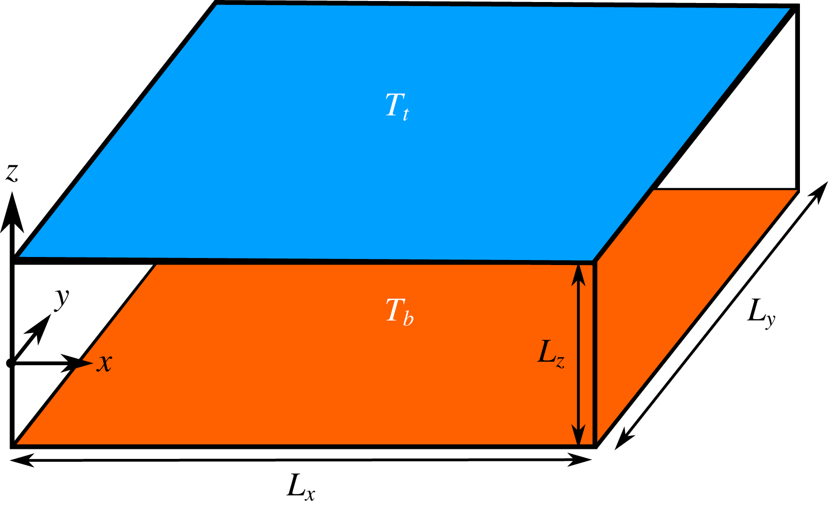
The 3D RBC system. The temperature at the top (bottom) wall is held at
 $T_{t}$
(
 $T_{b}$
), and
 $\unicode[STIX]{x0394}T=T_{b}-T_{t}>0$
. The horizontal directions (
 $x$
–
 $y$
) are periodic. The no-slip boundary condition is enforced at the walls. Here,
 $L_{x}=L_{y}=\unicode[STIX]{x03C0}L_{z}$
, the Prandtl number is
 $Pr=0.707$
and
 $Ra=10^{6}$
.

As a result, it is worthwhile to further examine the performance of
 $\unicode[STIX]{x1D647}_{FDT}$
in the context of a canonical fully turbulent flow system and explore whether basis functions other than POD modes can improve the performance of the FDT for developing ROMs for high-dimensional systems. Along these lines, the purpose of this study is twofold.
(1) To examine the performance of the FDT in calculating
 $\unicode[STIX]{x1D647}$
for a fully turbulent flow, i.e. 3D Rayleigh–Bénard convection (RBC) at a Rayleigh number of
$Ra=10^{6}$
(figure 1). Direct numerical simulation (DNS) of RBC, a fitting prototype for buoyancy-driven turbulence, is used to generate the data for the FDT.
(2) To show that the use of DMD modes, rather than the commonly used POD modes (also known as EOF modes), as the basis functions in the FDT calculation can resolve the problem previously identified in Hassanzadeh & Kuang (Reference Hassanzadeh and Kuang2016b ) and remarkably improve the performance of the FDT applied to high-dimensional turbulent systems.


Furthermore, this work aims to better connect the seemingly independent advances in the fluid dynamics and climate science communities. It is worth mentioning here, and further discussing in § 2, that the FDT and DMD are not unrelated. In fact, another method, called linear inverse modelling (LIM; Penland Reference Penland1989), that is also derived from the Fokker–Planck equation and is closely related to the FDT is, as pointed out by Tu et al. (Reference Tu, Rowley, Luchtenburg, Brunton and Kutz2014), mathematically equivalent to DMD, although LIM and DMD are derived using different concepts. These connections are not surprising given that the Koopman operator is the adjoint of the Perron–Frobenius operator (Klus, Koltai & Schütte Reference Klus, Koltai and Schütte2016) and that the latter is connected to the Fokker–Planck equation (Lasota & Mackey Reference Lasota and Mackey2013).
This paper is structured as follows. The formulations of the FDT and DMD are discussed in § 2. The 3D RBC system, its ROM and the DNS solver are described in § 3. In § 4, the accuracy of
 $\unicode[STIX]{x1D647}$
in predicting the time-mean response to forcing is examined for the FDT with basis functions of POD modes (
 $\text{FDT}_{POD}$
) and DMD modes (
 $\text{FDT}_{DMD}$
) using DNS of RBC and stochastic ODEs (SDEs). A summary and future work are discussed in § 5.
2 The FDT and DMD
Let
 $\boldsymbol{x}_{t}\in \mathbb{R}^{m}$
be time-mean-removed measurements (e.g. from DNS data) of the state vector (which might involve velocity and temperature) over
 $m$
grid points at time
 $t$
, and
 $$\begin{eqnarray}\displaystyle \unicode[STIX]{x1D653}_{o}=\{\boldsymbol{x}_{\unicode[STIX]{x0394}t}\;\;\boldsymbol{x}_{2\unicode[STIX]{x0394}t}\;\ldots \;\boldsymbol{x}_{N\unicode[STIX]{x0394}t}\},\quad \unicode[STIX]{x1D653}_{\unicode[STIX]{x1D70F}}=\{\boldsymbol{x}_{\unicode[STIX]{x1D70F}+\unicode[STIX]{x0394}t}\;\;\boldsymbol{x}_{\unicode[STIX]{x1D70F}+2\unicode[STIX]{x0394}t}\;\ldots \;\boldsymbol{x}_{\unicode[STIX]{x1D70F}+N\unicode[STIX]{x0394}t}\}, & & \displaystyle\end{eqnarray}$$
where
 $\unicode[STIX]{x0394}t$
is the sampling interval and
 $N$
is the number of samples. Therefore,
 $\unicode[STIX]{x1D653}_{0}$
and
 $\unicode[STIX]{x1D653}_{\unicode[STIX]{x1D70F}}$
are
 $m\times N$
matrices. Below, we present the mathematical formulation and numerical procedure for calculating
 $\unicode[STIX]{x1D647}$
from matrices like
 $\unicode[STIX]{x1D653}_{o}$
and
 $\unicode[STIX]{x1D653}_{\unicode[STIX]{x1D70F}}$
using the FDT, LIM and DMD. It is more convenient to start with the latter.
2.1 The DMD and LIM
Following the exact DMD formulation of Tu et al. (Reference Tu, Rowley, Luchtenburg, Brunton and Kutz2014), the operator
 $\unicode[STIX]{x1D63C}_{DMD}=\exp (\unicode[STIX]{x1D647}_{DMD}\unicode[STIX]{x1D70F})$
is calculated as
 $$\begin{eqnarray}\displaystyle \unicode[STIX]{x1D63C}_{DMD}=\unicode[STIX]{x1D653}_{\unicode[STIX]{x1D70F}}\unicode[STIX]{x1D653}_{o}^{+}. & & \displaystyle\end{eqnarray}$$
Here,
 $+$
denotes the pseudoinverse. The DMD modes (values) are the eigenvectors (values) of
 $\unicode[STIX]{x1D63C}_{DMD}$
. In practice, one often uses
 $\unicode[STIX]{x1D70F}=\unicode[STIX]{x0394}t$
and calculates the reduced singular value decomposition (SVD)
 $\unicode[STIX]{x1D653}_{o}=\unicode[STIX]{x1D650}\unicode[STIX]{x1D64E}\unicode[STIX]{x1D651}^{\dagger }$
and then
 $\unicode[STIX]{x1D63C}_{DMD}=\unicode[STIX]{x1D650}^{\dagger }\unicode[STIX]{x1D653}_{\unicode[STIX]{x1D70F}}\unicode[STIX]{x1D651}\unicode[STIX]{x1D64E}^{-1}$
, where
 $\dagger$
denotes the adjoint. It should be noted that some of the DMD modes might be complex; when we later choose a subset of DMD modes as basis functions, we ensure that the complex conjugate of any chosen complex DMD mode is also included (see § 4.3 for more details).
Penland (Reference Penland1989) showed that the operator
 $\unicode[STIX]{x1D63C}_{LIM}=\exp (\unicode[STIX]{x1D647}_{LIM}\unicode[STIX]{x1D70F})$
can be calculated, from the Fokker–Planck equation, as
 $$\begin{eqnarray}\displaystyle \unicode[STIX]{x1D63C}_{LIM}=\unicode[STIX]{x1D63E}_{\unicode[STIX]{x1D70F}}\unicode[STIX]{x1D63E}_{o}^{-1}, & & \displaystyle\end{eqnarray}$$
where
 $\unicode[STIX]{x1D63E}_{\unicode[STIX]{x1D70F}}=\unicode[STIX]{x1D653}_{\unicode[STIX]{x1D70F}}\unicode[STIX]{x1D653}_{o}^{\dagger }$
is the lag-
 $\unicode[STIX]{x1D70F}$
covariance matrix. In practice, for high-dimensional systems, covariance matrices are nearly singular (i.e. ill-conditioned), because often not enough data are available to accurately characterize a system that has a large number of degrees of freedom (i.e. the dataset is short). To overcome this problem, a common regularization strategy is to first project
 $\boldsymbol{x}_{t}$
onto the leading
 $r$
POD/EOF modes (obtained from SVD of
 $\unicode[STIX]{x1D653}_{o}$
) and perform the calculations in (2.3) in this reduced space. The value of
 $r$
is chosen such that the retained POD modes represent at least 95 % (or even 99 %) of the variance (Penland Reference Penland1989; Ring & Plumb Reference Ring and Plumb2008; Lutsko et al.
Reference Lutsko, Held and Zurita-Gotor2015).
It should be noted that because
 $\unicode[STIX]{x1D653}_{\unicode[STIX]{x1D70F}}\unicode[STIX]{x1D653}_{o}^{+}=\unicode[STIX]{x1D653}_{\unicode[STIX]{x1D70F}}(\unicode[STIX]{x1D653}_{o}^{\dagger }(\unicode[STIX]{x1D653}_{o}\unicode[STIX]{x1D653}_{o}^{\dagger })^{-1})=\unicode[STIX]{x1D63E}_{\unicode[STIX]{x1D70F}}\unicode[STIX]{x1D63E}_{o}^{-1}$
, (2.2) and (2.3) are equivalent; see Tu et al. (Reference Tu, Rowley, Luchtenburg, Brunton and Kutz2014) for further discussion. It should be pointed out that the Koopman operator, which describes the evolution of observables, and Perron–Frobenius operator, which describes the transition density function, are adjoints (e.g. Klus et al.
Reference Klus, Koltai and Schütte2016), and that if the stochastic noise vanishes, the Fokker–Planck operator reduces to the Perron–Frobenius operator; see, e.g., Lasota & Mackey (Reference Lasota and Mackey2013, chap. 11) and Giannakis (Reference Giannakis2017).
2.2 The FDT
According to the FDT (Kubo Reference Kubo1966; Leith Reference Leith1975), the linear response function can be calculated as
 $$\begin{eqnarray}\displaystyle \unicode[STIX]{x1D647}_{FDT}=-\left[\int _{0}^{\infty }\unicode[STIX]{x1D63E}_{\unicode[STIX]{x1D70F}}\unicode[STIX]{x1D63E}_{0}^{-1}\,\text{d}\unicode[STIX]{x1D70F}\right]^{-1}. & & \displaystyle\end{eqnarray}$$
It should be noted that the integrand is basically
 $\unicode[STIX]{x1D63C}_{DMD}$
or
 $\unicode[STIX]{x1D63C}_{LIM}$
, consistent with integrating
 $\unicode[STIX]{x1D63C}=\exp (\unicode[STIX]{x1D647}\unicode[STIX]{x1D70F})$
over
 $\unicode[STIX]{x1D70F}$
from 0 to
 $\infty$
if
 $\unicode[STIX]{x1D647}$
only has decaying modes. For details of the derivation of (2.4) from the Fokker–Planck equation see Majda et al. (Reference Majda, Abramov and Grote2005) and Gritsun & Branstator (Reference Gritsun and Branstator2007). It is of particular interest to find
 $\unicode[STIX]{x1D647}_{FDT}$
, because it allows calculation of the time-mean response to an imposed forcing or the forcing needed for a specified response via
 $\unicode[STIX]{x1D647}_{FDT}\langle \boldsymbol{x}\rangle =-\langle \,\boldsymbol{f}\rangle$
, where
 $\langle \,\rangle$
denotes long-time averaging. It should be noted that the key underlying assumption for the applicability of
 $\unicode[STIX]{x1D647}_{FDT}$
is not that the system is linear, but that the forcing is weak enough such that the response of the nonlinear system changes linearly with the forcing (Gritsun & Branstator Reference Gritsun and Branstator2007; Cooper & Haynes Reference Cooper and Haynes2011).
In practice, similarly to LIM, the calculations required to evaluate the expression appearing in (2.4) are typically carried out in the reduced space of the leading
 $r$
POD modes to avoid singular covariance matrices. The upper bound of the integral is also replaced with a finite limit
 $\unicode[STIX]{x1D70F}_{\infty }$
. The reason(s) behind the inaccuracy of
 $\unicode[STIX]{x1D647}_{FDT}$
calculated for high-dimensional systems (see § 1) is not fully understood, and often attributed to a number of potential fundamental and practical issues. For example, (2.4) (and (2.3)) is exact only if the statistics of
 $\boldsymbol{x}$
is Gaussian (Majda et al.
Reference Majda, Abramov and Grote2005; Gritsun & Branstator Reference Gritsun and Branstator2007), which is not the case for turbulent flows such as atmospheric circulation (Cooper & Haynes Reference Cooper and Haynes2011; Hassanzadeh, Kuang & Farrell Reference Hassanzadeh, Kuang and Farrell2014). Examples of practical issues include unsuitable choices of
 $r$
or
 $\unicode[STIX]{x1D70F}_{\infty }$
, short datasets and shortcomings of POD modes as basis functions (Cooper, Esler & Haynes Reference Cooper, Esler and Haynes2013; Hassanzadeh & Kuang Reference Hassanzadeh and Kuang2016b
). The latter issue is particularly significant and is addressed in the current study. However, first, we describe in § 3 the DNS dataset that is used for calculating matrices in (2.1).
3 The 3D RBC mathematical model, DNS solver and 1D ROM
The RBC system of figure 1 is modelled using the 3D Boussinesq equations. Choosing the height
 $L_{z}$
, temperature
 $\unicode[STIX]{x0394}T=T_{b}-T_{t}$
and diffusive time scale
 $\unicode[STIX]{x1D70F}_{diff}=L_{z}^{2}/\unicode[STIX]{x1D705}$
(
 $\unicode[STIX]{x1D705}$
is the thermal diffusivity) as characteristic scales, the dimensionless equations are
 $$\begin{eqnarray}\displaystyle & \unicode[STIX]{x1D735}^{\ast }\boldsymbol{\cdot }\boldsymbol{u}^{\ast }=0, & \displaystyle\end{eqnarray}$$
 $$\begin{eqnarray}\displaystyle & \displaystyle \frac{\unicode[STIX]{x2202}\boldsymbol{u}^{\ast }}{\unicode[STIX]{x2202}t^{\ast }}+(\boldsymbol{u}^{\ast }\boldsymbol{\cdot }\unicode[STIX]{x1D735}^{\ast })\boldsymbol{u}^{\ast }=-\unicode[STIX]{x1D735}^{\ast }p^{\ast }+Pr\,\unicode[STIX]{x1D6FB}^{\ast 2}\boldsymbol{u}^{\ast }+Ra\,Pr(T^{\ast }-T_{cond}^{\ast })\hat{\boldsymbol{e}}_{z}, & \displaystyle\end{eqnarray}$$
 $$\begin{eqnarray}\displaystyle & \displaystyle \frac{\unicode[STIX]{x2202}T^{\ast }}{\unicode[STIX]{x2202}t^{\ast }}+(\boldsymbol{u}^{\ast }\boldsymbol{\cdot }\unicode[STIX]{x1D735}^{\ast })T^{\ast }=\unicode[STIX]{x1D6FB}^{\ast 2}T^{\ast }, & \displaystyle\end{eqnarray}$$
where
 $\boldsymbol{u}^{\ast }$
,
 $T^{\ast }$
and
 $T_{cond}^{\ast }=1/2-z^{\ast }$
are the 3D velocity field, temperature and conduction temperature profile respectively. The superscript
 $\ast$
indicates dimensionless variables and operators. We define the Rayleigh and Prandtl numbers as
 $Ra=(g\unicode[STIX]{x1D6FC}\unicode[STIX]{x0394}TL_{z}^{3})/(\unicode[STIX]{x1D708}\unicode[STIX]{x1D705})$
and
 $Pr=\unicode[STIX]{x1D708}/\unicode[STIX]{x1D705}$
, where
 $g$
,
 $\unicode[STIX]{x1D6FC}$
and
 $\unicode[STIX]{x1D708}$
are the gravitational acceleration, and thermal expansion coefficient and kinematic viscosity of the fluid respectively.
Equations (3.1)–(3.3) for the system shown in figure 1 are simulated (at
 $Ra=10^{6}$
) using a pseudospectral Fourier–Fourier–Chebyshev DNS solver with a resolution of
 $128\times 128\times 129$
(see Khodkar et al. (Reference Khodkar, Hassanzadeh, Saleh and Grover2018) for more detail). The spatio-temporal analysis of the DNS data in Khodkar et al. (Reference Khodkar, Hassanzadeh, Saleh and Grover2018) shows that the flow is fully turbulent at this Rayleigh number, which is around 585 times higher than the critical Rayleigh number for the onset of linear instability.
As shown in Khodkar et al. (Reference Khodkar, Hassanzadeh, Saleh and Grover2018), a 1D ROM in the form of (1.1) can be formulated for this 3D RBC system,
 $$\begin{eqnarray}\dot{\overline{\unicode[STIX]{x1D703}}}=\unicode[STIX]{x1D647}\,\overline{\unicode[STIX]{x1D703}}+\overline{f},\end{eqnarray}$$
where the overbar indicates horizontal (
 $x$
–
 $y$
) averaging. Here, the state vector
 $\boldsymbol{x}=\overline{\unicode[STIX]{x1D703}}(z,t)$
is the response of the horizontally averaged temperature to external forcing
 $\overline{f}(z,t)$
, i.e. the deviation from the long-time-mean horizontally averaged temperature of the unforced system (hereafter, ‘unforced’ systems refer to (3.1)–(3.3); in the forced systems, an external forcing
 $f$
is added to (3.3)). Here, ‘1D’ highlights that the ROM describes the system in only one spatial direction,
 $z$
, as the state vector is horizontally averaged. The linear response function
 $\unicode[STIX]{x1D647}$
in (3.4) includes the vertical heat flux by molecular diffusion as well as vertical eddy heat flux. Because of the latter,
 $\unicode[STIX]{x1D647}$
cannot be derived directly from (3.1)–(3.3). Khodkar et al. (Reference Khodkar, Hassanzadeh, Saleh and Grover2018) showed that
 $\unicode[STIX]{x1D647}$
can be accurately calculated using the Green’s function (GRF) method (Kuang Reference Kuang2010; Hassanzadeh & Kuang Reference Hassanzadeh and Kuang2016a
), which requires many forced DNS of (3.1)–(3.3). As demonstrated in § 4, using the FDT,
 $\unicode[STIX]{x1D647}$
in (3.4) can be accurately calculated from a dataset obtained from unforced DNS.
4 Results
4.1 The DNS of RBC at
$Ra=10^{6}$
:
$\text{FDT}_{POD}$


From DNS of the unforced system, after the flow reaches quasi-equilibrium,
 $N=1.1\times 10^{5}$
samples of
 $\overline{T}(z,t)-\langle \overline{T}\rangle (z)$
are collected every
 $\unicode[STIX]{x0394}t=0.12\unicode[STIX]{x1D70F}_{adv}$
, where
 $\unicode[STIX]{x1D70F}_{adv}=\sqrt{L_{z}/(g\unicode[STIX]{x1D6FC}\unicode[STIX]{x0394}T)}$
is the advective time scale. As stated in Khodkar et al. (Reference Khodkar, Hassanzadeh, Saleh and Grover2018), in this system,
 $\unicode[STIX]{x1D70F}_{adv}=0.4\unicode[STIX]{x1D70F}_{d}=0.0012\unicode[STIX]{x1D70F}_{diff}$
, where
 $\unicode[STIX]{x1D70F}_{d}$
is the decorrelation time of the leading POD mode (POD1). Using these data,
 $\unicode[STIX]{x1D647}_{FDT_{POD}}$
is calculated from (2.4) for various values of
 $r$
and
 $\unicode[STIX]{x1D70F}_{\infty }$
. Several tests involving prediction of the time-mean response to an external forcing or the forcing needed for a specific time-mean response are used to evaluate the accuracy of the calculated
 $\unicode[STIX]{x1D647}_{FDT_{POD}}$
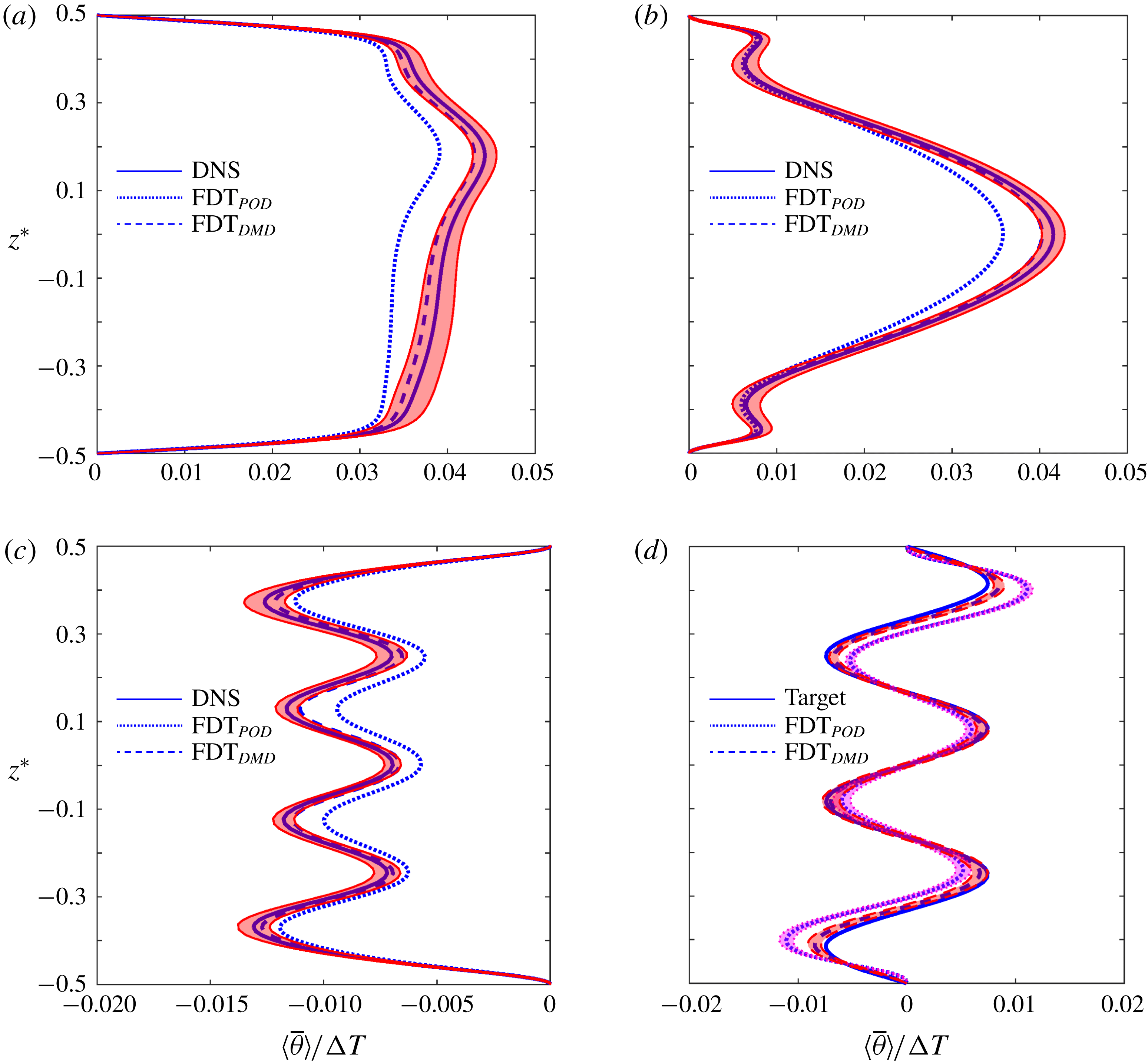
. The ‘true’ responses or forcings for these tests are obtained using DNS of forced systems. Figure 2 depicts the results for four of these tests.
Time-mean responses
 $\langle \overline{\unicode[STIX]{x1D703}}\rangle$
to forcings in the form of
 $f_{i}=(\unicode[STIX]{x0394}T/\unicode[STIX]{x1D70F}_{diff})\hat{f}_{i}$
: (a)
 $\hat{f_{1}}=10\exp [-(z^{\ast }-0.2)^{2}/0.1^{2}]$
, (b)
 $\hat{f_{2}}=20\cos (2\unicode[STIX]{x03C0}z^{\ast })$
, (c)
 $\hat{f_{3}}=20\cos (8\unicode[STIX]{x03C0}z^{\ast })$
. To quantify the ‘true’ responses and their uncertainty, each long forced DNS dataset is divided into eight equal segments and solid lines (red shading) show their mean (
 $\pm 1$
standard deviation). Dotted (dashed) lines show
 $-\unicode[STIX]{x1D647}_{FDT_{POD}}^{-1}f_{i}$
(
 $-\unicode[STIX]{x1D647}_{FDT_{DMD}}^{-1}f_{i}$
) where the optimal values of
 $(r,\unicode[STIX]{x1D70F}_{\infty }/\unicode[STIX]{x1D70F}_{d})=(20,0.833)$
are used in (2.4) (see the text). (d) The inverse problem: the forcing needed for a specified time-mean response
 $\langle \overline{\unicode[STIX]{x1D703}}\rangle _{target}$
(solid line) is calculated as
 $-\unicode[STIX]{x1D647}_{FDT_{POD}}\langle \overline{\unicode[STIX]{x1D703}}\rangle _{target}$
and
 $-\unicode[STIX]{x1D647}_{FDT_{POD}}\langle \overline{\unicode[STIX]{x1D703}}\rangle _{target}$
. To examine the accuracy, long DNS with these forcings is conducted, and the dashed/dotted lines show the calculated
 $\langle \overline{\unicode[STIX]{x1D703}}\rangle$
.

As shown in figure 2(a–c),
 $\unicode[STIX]{x1D647}_{FDT_{POD}}$
predicts the pattern of the time-mean responses well, but generally over- or underestimates the amplitudes. Figure 2(d) demonstrates the accuracy of
 $\unicode[STIX]{x1D647}_{FDT_{POD}}$
for the inverse problem (i.e. flow control): prediction of the forcing needed to produce a specified change in the time-mean flow (i.e. a target response). As before, the FDT-predicted forcing can produce the pattern of the target reasonably well, but the amplitude is incorrect. The results presented in this figure are calculated using the optimal
 $(r,\unicode[STIX]{x1D70F}_{\infty })$
, obtained from exploring the accuracy of the predicted responses/forcings in each case over a range of these two parameters (figure 3). We find that for all tests,
 $(r=20,\unicode[STIX]{x1D70F}_{\infty }=0.83\unicode[STIX]{x1D70F}_{d})$
is optimal and leads to the closest agreement with the truth (i.e. DNS). These results suggest that for the best accuracy at
 $N=1.1\times 10^{5}$
, independent of the forcing, the spatial dimension of the original samples
 $\boldsymbol{x}_{t}$
(
 $m=129$
) should be reduced to
 $r=20$
, and that
 $\unicode[STIX]{x1D70F}_{\infty }$
, which the accuracy is notably sensitive to, should be chosen slightly less than the decorrelation time of POD1 (
 $\unicode[STIX]{x1D70F}_{d}$
). The latter is consistent with the findings of Gritsun & Branstator (Reference Gritsun and Branstator2007) and Hassanzadeh & Kuang (Reference Hassanzadeh and Kuang2016b
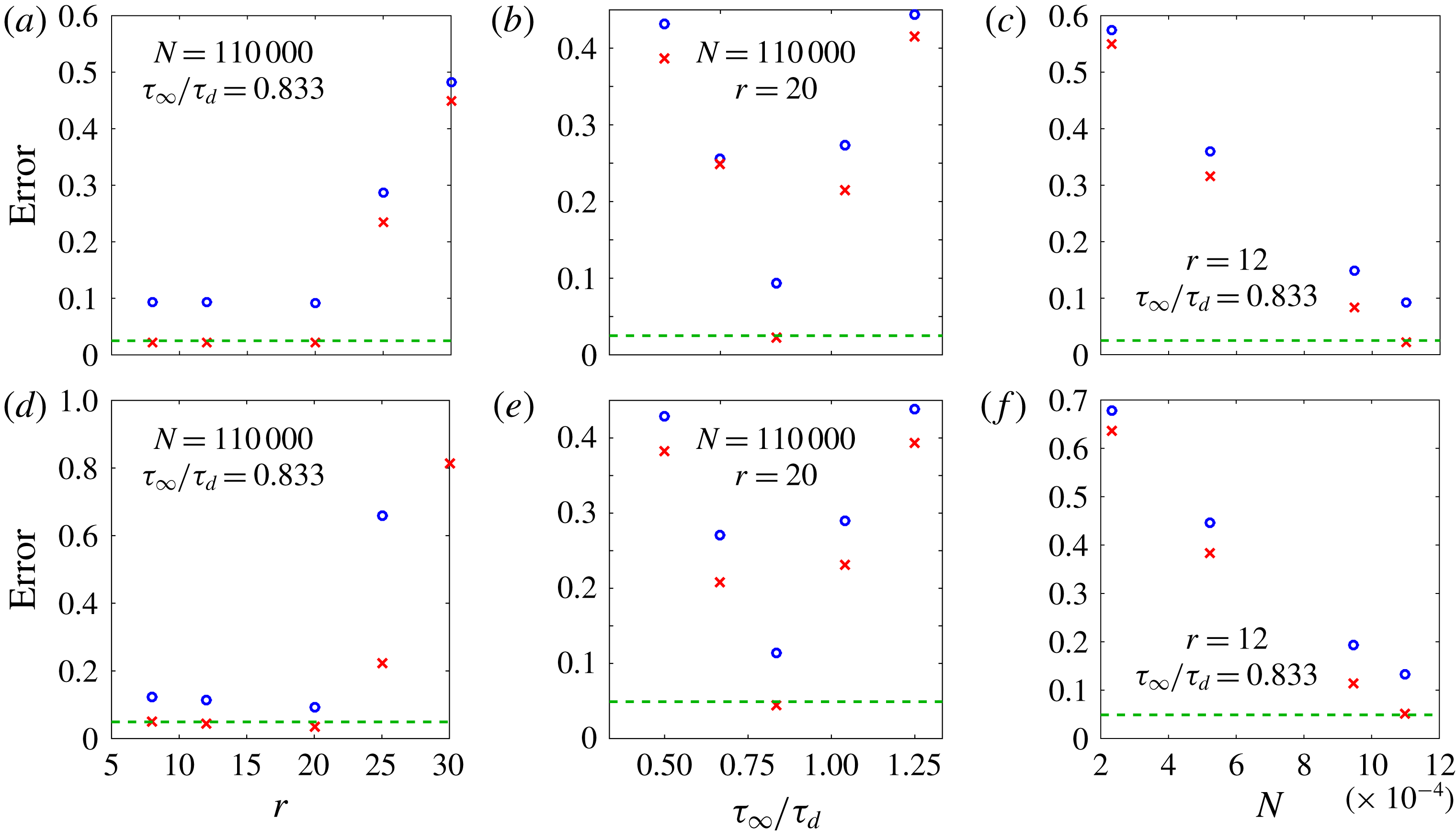
) in climate models. Figure 3(c,f) shows how the accuracy improves by increasing
 $N$
.
The accuracy of
 $\unicode[STIX]{x1D647}_{FDT}$
in predicting the response
 $\langle \overline{\unicode[STIX]{x1D703}}\rangle$
to forcings
 $f_{1}$
(a–c) and
 $f_{2}$
(d–f), as functions of the number of leading POD or DMD modes used in the projection
 $r$
(a,d),
 $\unicode[STIX]{x1D70F}_{\infty }/\unicode[STIX]{x1D70F}_{d}$
(b,e) and the length of the dataset
 $N$
(c,f). The values of other parameters that are maintained constant can be seen in each panel. The blue circles and red crosses correspond to
 $\text{FDT}_{POD}$
and
 $\text{FDT}_{DMD}$
respectively. Since for the short datasets, the number of well-captured POD or DMD modes does not exceed 12, we have used
 $r=12$
in (c) and (f) for the sake of a fair comparison. The horizontal dashed lines show the errors of
 $\unicode[STIX]{x1D647}_{GRF}$
from Khodkar et al. (Reference Khodkar, Hassanzadeh, Saleh and Grover2018). Errors are calculated as
 ${\Vert \langle \overline{\unicode[STIX]{x1D703}}\rangle _{\unicode[STIX]{x1D647}}-\langle \overline{\unicode[STIX]{x1D703}}\rangle _{DNS}\Vert }_{2}/{\Vert \langle \overline{\unicode[STIX]{x1D703}}\rangle _{DNS}\Vert }_{2}$
.

The results shown in figures 2 and 3 (and more tests, not shown) are promising, particularly given that the flow is complex and fully turbulent. However, the performance of
 $\unicode[STIX]{x1D647}_{FDT_{POD}}$
is still not fully satisfactory as the predicted amplitudes are inaccurate and the
 $\text{FDT}_{POD}$
is substantially outperformed by the accurate but computationally demanding (and not model-free) GRF method. An analysis by Khodkar et al. (Reference Khodkar, Hassanzadeh, Saleh and Grover2018) based on evaluation of the
 $\unicode[STIX]{x1D716}$
-pseudospectrum showed that the RBC system under consideration here is moderately non-normal (see their figure 10b), which suggests that the performance of
 $\unicode[STIX]{x1D647}_{FDT_{POD}}$
might be suffering from the same problem as identified in Hassanzadeh & Kuang (Reference Hassanzadeh and Kuang2016b
): use of the leading
 $r$
POD modes, which are orthogonal, can significantly degrade the performance of
 $\text{FDT}_{POD}$
if the system is non-normal, even if the
 $r\,({<}m)$
modes explain a large percentage of the variance. This problem, and a potential remedy based on using DMD rather than POD modes for basis functions, is best seen by considering simple
 $2\times 2$
systems of SDEs. This is done below, followed by application of
 $\text{FDT}_{DMD}$
to the same DNS dataset in § 4.3.
4.2 Normal, non-normal and nonlinear SDEs:
$\text{FDT}_{POD}$
and
$\text{FDT}_{DMD}$


We consider a two-dimensional SDE,
 $$\begin{eqnarray}\dot{\boldsymbol{z}}=\unicode[STIX]{x1D63C}\,\boldsymbol{z}+\unicode[STIX]{x1D743}+\boldsymbol{f},\end{eqnarray}$$
where
 $\boldsymbol{z}^{\text{T}}=[z_{1}~z_{2}]$
,
 $\unicode[STIX]{x1D743}$
is Gaussian white noise and
 $\boldsymbol{f}$
is a constant forcing. We use three test cases that are respectively normal, non-normal and nonlinear, with
 $\unicode[STIX]{x1D63C}$
being
 $$\begin{eqnarray}\unicode[STIX]{x1D63C}_{1}=\left[\begin{array}{@{}cc@{}}-1 & 0\\ 0 & -2\end{array}\right],\quad \unicode[STIX]{x1D63C}_{2}=\left[\begin{array}{@{}cc@{}}-1 & 5\\ 0 & -2\end{array}\right],\quad \unicode[STIX]{x1D63C}_{3}=\left[\begin{array}{@{}cc@{}}-1 & -4z_{2}+2\\ 0 & -2\end{array}\right].\end{eqnarray}$$
We remark that the same matrices
 $\unicode[STIX]{x1D63C}_{1}$
and
 $\unicode[STIX]{x1D63C}_{2}$
were used in Hassanzadeh & Kuang (Reference Hassanzadeh and Kuang2016b
) for a similar analysis which was focused only on POD modes. Setting
 $\boldsymbol{f}=0$
, the SDE for each test case is integrated using the Euler–Maruyama method to generate datasets with 30 000 samples of
 $\boldsymbol{z}_{t}$
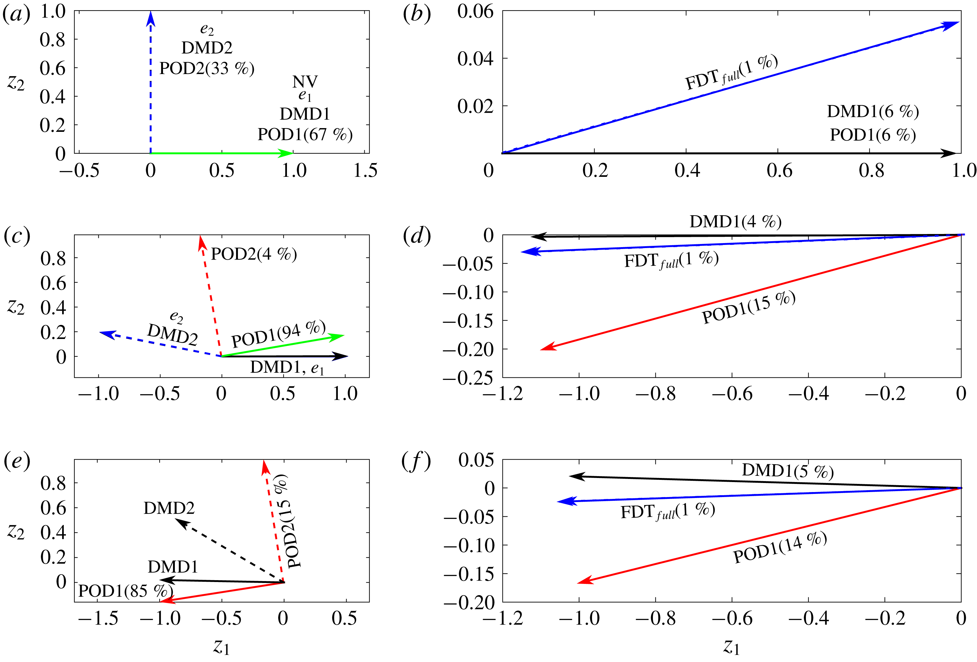
. The POD and DMD modes are calculated from these datasets following § 2 and shown in figure 4. As expected, for
 $\unicode[STIX]{x1D63C}_{1}$
, the POD and DMD modes and eigenvectors are all identical (and each orthogonal), while for
 $\unicode[STIX]{x1D63C}_{2}$
, the DMD modes and eigenvectors are the same (and non-orthogonal) but different from the POD modes (which are orthogonal). For
 $\unicode[STIX]{x1D63C}_{3}$
, the DMD and POD modes differ.
(a,c,e) Eigenvectors
 $\boldsymbol{e}$
(blue lines), DMD modes (black lines) and POD modes (red lines) for the systems with
 $\unicode[STIX]{x1D63C}_{1}$
(a,b),
 $\unicode[STIX]{x1D63C}_{2}$
(c,d) and
 $\unicode[STIX]{x1D63C}_{3}$
(e,f). Here,
 $\boldsymbol{e}_{1}$
and DMD1 are the slower-decaying modes. The percentages show the variance explained by each POD mode. (b,d,f) Time-mean response to the forcing
 $(0.9\text{POD}1+0.1\text{POD}2)/\Vert 0.9\text{POD}1+0.1\text{POD}2\Vert _{2}$
, calculated using the FDT (2.4) with no projection (
 $\text{FDT}_{full}$
; dashed blue lines), and projection onto the leading POD (
 $\text{FDT}_{POD1}$
; red lines) or DMD (
 $\text{FDT}_{DMD1}$
; black lines) mode. The solid blue lines show the analytically or numerically calculated true responses. The percentages show errors computed as
 ${\Vert \boldsymbol{z}_{FDT}-\boldsymbol{z}_{true}\Vert }_{2}\times 100/{\Vert \boldsymbol{z}_{true}\Vert }_{2}$
. It should be noted that the ranges of the axes vary among panels.

Time-mean responses to an external forcing
 $\boldsymbol{f}$
that is mostly in the direction of POD1 but has a small projection onto POD2 are predicted using
 $\unicode[STIX]{x1D647}_{FDT}$
when no truncation is performed (
 $\text{FDT}_{full}$
) and when the data are truncated onto POD1 (
 $\text{FDT}_{POD1}$
). For all test cases,
 $\text{FDT}_{full}$
has an error of
 ${\sim}1\,\%$
. While for the normal system
 $\text{FDT}_{POD1}$
is relatively accurate (error
 ${\sim}6\,\%$
), for the non-normal system the error is around 15 % even though POD1 explains 94 % of the variance. To explain the source of this inaccuracy, following Hassanzadeh & Kuang (Reference Hassanzadeh and Kuang2016b
), we transfer (4.1) to the basis function space,
 $$\begin{eqnarray}\dot{\boldsymbol{a}}=[\unicode[STIX]{x1D63D}^{-1}(\unicode[STIX]{x1D640}\unicode[STIX]{x1D726}\unicode[STIX]{x1D640}^{-1})\unicode[STIX]{x1D63D}]\boldsymbol{a}+\unicode[STIX]{x1D63D}^{-1}\boldsymbol{f},\end{eqnarray}$$
where
 $\boldsymbol{a}^{\text{T}}=[a_{1}~a_{2}]$
are the projection coefficients, columns of
 $\unicode[STIX]{x1D63D}$
contain the basis functions (e.g. POD modes),
 $\unicode[STIX]{x1D640}$
(
 $\unicode[STIX]{x1D726}$
) contain the eigenvectors (values) of
 $\unicode[STIX]{x1D63C}$
and
 $\unicode[STIX]{x1D743}$
is ignored for convenience. For a normal system, the POD modes are the same as the eigenvectors, and the matrix in the brackets reduces to the diagonal matrix
 $\unicode[STIX]{x1D726}$
, decoupling
 $a_{1}$
and
 $a_{2}$
. Projections of
 $\boldsymbol{f}$
onto POD2 cannot be captured if
 $\unicode[STIX]{x1D647}_{POD}$
is calculated only in the space of POD1; however, the accuracy of
 $a_{1}$
will not be affected, leading to the small error in figure 4(b). For non-normal systems, the POD modes and eigenvectors can be significantly different, leading to a coupling between
 $a_{1}$
and
 $a_{2}$
that strengthens with non-normality (Hassanzadeh & Kuang Reference Hassanzadeh and Kuang2016b
). Hence, even small projections of
 $\boldsymbol{f}$
onto POD2 can substantially degrade the accuracy of
 $a_{1}$
(and thus the FDT prediction) if
 $\unicode[STIX]{x1D647}_{FDT}$
is calculated only in the space of POD1 (figure 4
d).
The above analysis suggests that the use of basis functions that approximate the system eigenvectors might improve the accuracy of
 $\unicode[STIX]{x1D647}_{FDT}$
. The discussion in § 2 and the results in figure 4 point to DMD modes as potential options. Indeed, use of the slower-decaying DMD mode as the basis function (
 $\text{FDT}_{DMD1}$
hereafter) improves the accuracy compared with
 $\text{FDT}_{POD1}$
by a factor of four for the non-normal system. Similarly, in the nonlinear system, the error of
 $\text{FDT}_{DMD1}$
is 5 %, three times lower than the 15 % error of
 $\text{FDT}_{POD1}$
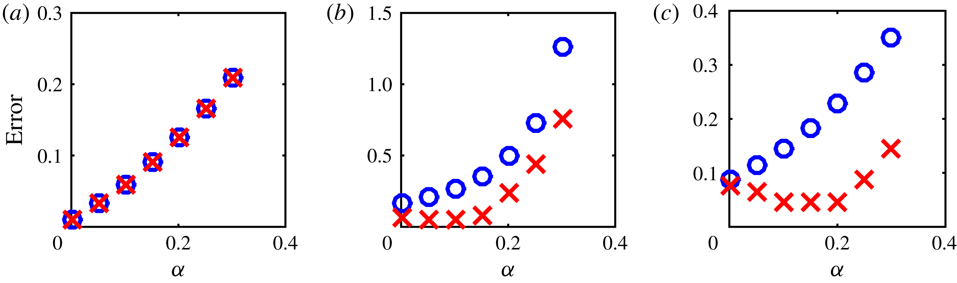
. To further demonstrate the advantage of using the leading DMD rather than POD mode as the basis function, figure 5 shows that as the projection of the forcing onto POD2 increases in the non-normal and nonlinear systems, the accuracy of FDT-predicted responses rapidly degrades for
 $\text{FDT}_{POD1}$
while
 $\text{FDT}_{DMD1}$
shows a much better performance.
For systems with (a)
 $\unicode[STIX]{x1D63C}_{1}$
, (b)
 $\unicode[STIX]{x1D63C}_{2}$
and (c)
 $\unicode[STIX]{x1D63C}_{3}$
, errors in time-mean response predictions to forcing
 $[(1-\unicode[STIX]{x1D6FC})\text{POD}1+\unicode[STIX]{x1D6FC}\text{POD}2]/\Vert (1-\unicode[STIX]{x1D6FC})\text{POD}1+\unicode[STIX]{x1D6FC}\text{POD}2\Vert _{2}$
. The blue circles and red crosses indicate
 $\text{FDT}_{POD1}$
and
 $\text{FDT}_{DMD1}$
respectively. The error is computed as
 ${\Vert \boldsymbol{z}_{FDT}-\boldsymbol{z}_{true}\Vert }_{2}/{\Vert \boldsymbol{z}_{true}\Vert }_{2}$
. It should be noted that the range of the
 $y$
-axis varies among panels.

4.3 The DNS of RBC at
$Ra=10^{6}$
:
$\text{FDT}_{DMD}$


Using the unforced system DNS, we have calculated, following § 2.1 for
 $\unicode[STIX]{x1D70F}=\unicode[STIX]{x0394}t$
, all of the
 $m=129$
DMD modes, and chosen the
 $r$
slowest-decaying ones as basis functions for
 $\text{FDT}_{DMD}$
. If the
 $r\text{th}$
DMD mode is complex, we ensure that its complex conjugate, also a DMD mode, is included in the basis function space as well. Figures 2 and 3 show that
 $\unicode[STIX]{x1D647}_{FDT_{DMD}}$
accurately predicts the pattern and amplitude of the time-mean responses and remarkably outperforms
 $\unicode[STIX]{x1D647}_{FDT_{POD}}$
in all cases. The linear response function
 $\unicode[STIX]{x1D647}_{FDT_{DMD}}$
has an accuracy that is equal to (or in some cases better than) that of
 $\unicode[STIX]{x1D647}_{GRF}$
. It should be noted that while DMD modes provide suitable basis functions for the FDT, we have found that
 $\unicode[STIX]{x1D647}_{DMD}$
(or
 $\unicode[STIX]{x1D647}_{LIM}$
) cannot accurately predict the time-mean responses/forcings for tests similar to those in figure 2 (not shown).
5 Discussion and conclusions
The DMD-enhanced FDT method is shown to accurately predict the time-mean response to an external forcing, or the forcing needed for a specified response in a canonical buoyancy-driven turbulent flow, RBC at
 $Ra=10^{6}$
. Tests using the DNS of RBC and simple non-normal and nonlinear SDEs demonstrate the advantage in using a limited number of leading (slowest-decaying) DMD modes over the commonly used POD modes as basis functions for the FDT calculations in (2.4).
This approach suggests a potential remedy to overcome the challenge identified by Hassanzadeh & Kuang (Reference Hassanzadeh and Kuang2016b
) in applying the FDT to high-dimensional non-normal turbulent flows. Nonetheless, while the 1D linear ROM calculated using
 $\text{FDT}_{DMD}$
remarkably outperforms
 $\text{FDT}_{POD}$
and accurately predicts the pattern and amplitude of time-mean responses/forcings for the Rayleigh–Bénard turbulence considered here, how the DMD-enhanced FDT performs for computing 2D and 3D ROMs and for more complex higher-dimensional turbulent systems remains to be examined in future work. Large-scale atmospheric circulation, for which
 $\text{FDT}_{POD}$
has been extensively attempted with mixed outcomes, will be a test case of particular interest.
Finally, given the non-normality of the system, the sensitivity of the calculated responses to the initial condition in initial-value integrations of (3.4) and to small changes in the forcing (in both DNS and (3.4)) should be investigated in subsequent studies.
Acknowledgements
We thank T. Antoulas, H. Babaee, M. Farazmand, P. Grover, M. Heinkenschloss and S. Nabi for insightful discussions, three anonymous reviewers for helpful comments, NSF grant AGS-1552385, NASA grant 80NSSC17K0266 and Rice University’s Faculty Initiative Fund for support, and XSEDE Stampede2 (via allocation ATM170020) and Rice’s DAVinCI cluster for providing computing resources.