


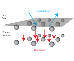


1 Introduction
The physical behaviour of a number of fluid systems is dramatically modified by the presence of a small-scale surface roughness. For example, in wetting (figure 1a) – that is, when a liquid in contact with a solid reaches a balance of surface tensions – the resulting apparent contact angle  $\unicode[STIX]{x1D703}$ is very sensitive to the details of the surface texture (Wenzel Reference Wenzel1936; Quéré Reference Quéré2008). At high Reynolds numbers (of order 1000 and above), the pressure loss in turbulent pipes is a function of the wall roughness (figure 1b) (Nikuradse Reference Nikuradse1950; Jiménez Reference Jiménez2004). Yet another example is the transport phenomena involving porous media, where the exchange of mass, momentum, energy and other passive scalars between a free flowing fluid and a porous medium depends very much on the roughness at the interface between the two domains (figure 1c).
Examples of problems that are sensitive to surface properties. Droplet spreading over a rough surface (a), friction drag of turbulent flow on a rough surface (b) and particle transport through the interface with a rough porous material (c).

Engineers take advantage of the sensitivity to the surface texture to modify large-scale flow features and to enhance the transport phenomena. Efficiency of heat exchangers (Mehendale, Jacobi & Shah Reference Mehendale, Jacobi and Shah2000; Agyenim et al. Reference Agyenim, Hewitt, Eames and Smyth2010) is highly dependent on the surface texture. In scaffold design for bone regeneration, the cell growth on the implant (a porous biomaterial such as a calcium phosphate cement) depends on the interaction between the surrounding liquid and the surface texture of the implant (Dalby et al. Reference Dalby, Gadegaard, Tare, Andar, Riehle, Herzyk, Wilkinson and Oreffo2007; Perez & Mestres Reference Perez and Mestres2016). The performance of fuel cells depends on the ability of gas flow to efficiently transport the water vapour away from the cathode, a thin porous medium (Prat Reference Prat2002; Haghighi & Kirchner Reference Haghighi and Kirchner2017). Turbulent skin friction on wings or turbine blades can be reduced by using riblets, which are able to push quasi-streamwise vortices away from the wall (Walsh & Lindemann Reference Walsh and Lindemann1984).
The design of the surface texture in the examples mentioned above is based on a trial and error procedure that may require a tremendous amount of effort, time and expensive surface manufacturing equipment. The formulation presented in this paper provides a framework for modelling the interaction between free flows and various textured and porous surfaces. Our modelling approach provides a direct relationship between the microscopic geometrical details of a complex surface and the associated macroscopic transport of mass and momentum. Thus it has the potential to replace the trial and error procedure in the design phase.
Due to the multiscale nature of the problems described above, fully resolved numerical investigations – of both the complex surface and the free flow above it – are practically impossible to perform in applied settings. Effective approaches are actively pursued to circumvent this difficulty. In this way, one can capture the averaged effect of the microscale features on the macroscopic processes, and hence avoid resolving microscopic geometric details. Some recent examples of effective modelling applied to drying, cell growth, heat exchange and flow modelling can be found in works by Mosthaf, Helmig & Or (Reference Mosthaf, Helmig and Or2014), Vaca-González et al. (Reference Vaca-González, Moncayo-Donoso, Guevara, Hata, Shefelbine and Garzón-Alvarado2018), Laloui, Nuth & Vulliet (Reference Laloui, Nuth and Vulliet2006), Wang et al. (Reference Wang, Zhang, Xiao, Jin and Li2018) and Zampogna et al. (Reference Zampogna, Lācis, Bagheri and Bottaro2019a). The main challenge for effective models describing fluid–surface interaction is the specification of a boundary condition at an artificially created interface between the free-fluid region and the complex surface. Despite the recent advancements, we still lack interface conditions that capture the dominant physical features associated with complex anisotropic surfaces.
Schematics of the slip length  $L$ (a), the transpiration length
 $M$ (b) and the resistance coefficient
 $f$ (c).

Before highlighting the main ingredients of our model, we make a brief account of the current state-of-the-art of effective boundary conditions of textured and porous surfaces. A two-dimensional configuration is sufficient for this purpose. The streamwise and wall-normal coordinates are denoted by  $x$ and
 $z$, where the effective boundary conditions are imposed at a planar interface at coordinate
 $z=z_{i}$. For rigid textured surfaces with a characteristic size
 $\ell$, one may impose the slip velocity condition (Navier Reference Navier1823) as an effective boundary condition,
 $$\begin{eqnarray}u_{x}=L(\unicode[STIX]{x2202}_{z}u_{x}+\unicode[STIX]{x2202}_{x}u_{z})\quad \text{on }z=z_{i}.\end{eqnarray}$$
Here,  $u_{x}$ is the tangential velocity component at the interface,
 $u_{z}$ is the wall-normal velocity component at the interface and
 $L\sim \ell$ is the slip length. Geometrically – as shown in figure 2(a) – the slip length in its simplest possible representation (i.e. assuming no variation in the
 $x$ direction) is the distance that the velocity profile has to be linearly extrapolated to reach zero value. There has been extensive development of the slip boundary condition for textured and porous surfaces (Saffman Reference Saffman1971; Sahraoui & Kaviany Reference Sahraoui and Kaviany1992; Miksis & Davis Reference Miksis and Davis1994; Sarkar & Prosperetti Reference Sarkar and Prosperetti1996; Gupte & Advani Reference Gupte and Advani1997; Jäger & Mikelić Reference Jäger and Mikelić2001; Stroock et al. Reference Stroock, Dertinger, Whitesides and Ajdari2002; Bolanos & Vernescu Reference Bolanos and Vernescu2017). In the existing approaches, the interface normal (transpiration) velocity is typically set either to zero
 $u_{z}=0$ (for textured surfaces) or to the interior flow
 $u_{z}=u_{z}^{-}$ (for porous surfaces) due to mass conservation arguments or as the leading-order boundary condition (Mohammadi & Floryan Reference Mohammadi and Floryan2013; Lācis & Bagheri Reference Lācis and Bagheri2016; Jiménez Bolaños & Vernescu Reference Jiménez Bolaños and Vernescu2017).
Configurations with porous surfaces require additional boundary conditions. If the bulk of the surface (i.e. interior of the porous material) is governed by the Darcy–Brinkmann equation, which is typical for works considering the method of volume averaging (Whitaker Reference Whitaker1998), stress jump conditions are often derived (Ochoa-Tapia & Whitaker Reference Ochoa-Tapia and Whitaker1995; Valdés-Parada et al. Reference Valdés-Parada, Alvarez-Ramírez, Goyeau and Ochoa-Tapia2009, Reference Valdés-Parada, Aguilar-Madera, Ochoa-Tapia and Goyeau2013). In the current work, however, we consider only Darcy’s law within the bulk of the porous surface. Consequently, a condition for the Darcy pressure or the pore pressure  $p^{-}$ is needed. The pressure continuity
 $p=p^{-}$, where
 $p$ is the free-fluid pressure, has been a common choice in the past (Ene & Sanchez-Palencia Reference Ene and Sanchez-Palencia1975; Levy & Sanchez-Palencia Reference Levy and Sanchez-Palencia1975; Hou et al. Reference Hou, Holmes, Lai and Mow1989; Lācis & Bagheri Reference Lācis and Bagheri2016). The most notable recent theoretical and numerical developments (Marciniak-Czochra & Mikelić Reference Marciniak-Czochra and Mikelić2012; Carraro et al. Reference Carraro, Goll, Marciniak-Czochra and Mikelić2013; Carraro, Marušić-Paloka & Mikelić Reference Carraro, Marušić-Paloka and Mikelić2018) have resulted in the pressure jump condition
 $$\begin{eqnarray}p^{-}-p=-\unicode[STIX]{x1D707}C_{\unicode[STIX]{x03C0}}\unicode[STIX]{x2202}_{z}u_{x}-2\unicode[STIX]{x1D707}\unicode[STIX]{x2202}_{z}u_{z}.\end{eqnarray}$$
Here,  $\unicode[STIX]{x1D707}$ is the fluid dynamic viscosity and
 $C_{\unicode[STIX]{x03C0}}$ is a stabilisation parameter derived from matching boundary layer solutions with exterior solutions. The coefficient
 $C_{\unicode[STIX]{x03C0}}$ is non-zero only for anisotropic porous surfaces. The pressure interface condition – as well as the velocity interface condition – for porous media has been a subject of many investigations and is still debated (Beavers & Joseph Reference Beavers and Joseph1967; Mikelić & Jäger Reference Mikelić and Jäger2000; Han, Ganatos & Weinbaum Reference Han, Ganatos and Weinbaum2005; Le Bars & Grae Worster Reference Le Bars and Grae Worster2006; Jäger & Mikelić Reference Jäger and Mikelić2009; Carraro et al. Reference Carraro, Goll, Marciniak-Czochra and Mikelić2015, Reference Carraro, Marušić-Paloka and Mikelić2018; Rosti, Cortelezzi & Quadrio Reference Rosti, Cortelezzi and Quadrio2015; Lācis & Bagheri Reference Lācis and Bagheri2016; Zampogna & Bottaro Reference Zampogna and Bottaro2016; Angot, Goyeau & Ochoa-Tapia Reference Angot, Goyeau and Ochoa-Tapia2017; Zampogna, Magnaudet & Bottaro Reference Zampogna, Magnaudet and Bottaro2019b).
In this work, we extend the above conditions with new terms for the wall-normal velocity condition and the pressure condition. Our proposed set of boundary conditions is called the transpiration-resistance (TR) model, and it is applicable to any textured or porous surface consisting of regular repeating geometric entities. The TR model captures the transport of interface tangential momentum as well as the transport of mass and interface normal momentum. It is a homogenised boundary condition, valid for configurations with a scale separation  $\unicode[STIX]{x1D716}=\ell /H\ll 1$, where
 $H$ is the characteristic length scale of the free fluid. It consists of the slip boundary condition (1.1) for the interface tangential velocity. The wall-normal velocity in the TR model is
 $$\begin{eqnarray}u_{z}=u_{z}^{-}-M\unicode[STIX]{x2202}_{x}u_{x}.\end{eqnarray}$$
The first term is the seepage Darcy velocity, given by  $u_{z}^{-}=(K/\unicode[STIX]{x1D707})\unicode[STIX]{x2202}_{z}p^{-}$, where
 $K$ is the interior permeability. The second term quantifies how much a surface texture allows exchange of mass with the surrounding fluid due to a streamwise variation of the slip velocity. Using continuity, the above condition for textured surfaces (where
 $u_{z}^{-}=0$) can be written as
 $u_{z}=M\unicode[STIX]{x2202}_{z}u_{z}$. Geometrically (figure 2b), the transpiration length
 $M$ is thus the distance below the interface for which a non-zero transpiration velocity
 $u_{z}$ can exist. This depth is obtained from a linear extrapolation of the wall-normal component of the outer flow,
 $u_{z}$. For a porous surface, the TR model provides the pressure condition,
 $$\begin{eqnarray}-p+2\unicode[STIX]{x1D707}\unicode[STIX]{x2202}_{z}u_{z}=-p^{-}+f\,u_{z}^{-}.\end{eqnarray}$$
Here, the left-hand side is the normal stress of the outside free flow on the interface plane, and the right-hand side is the normal stress from the porous material. The resistance coefficient  $f$ quantifies the friction force that the Darcy seepage velocity generates while passing through the interface (figure 2c).
Three assumptions underlie the proposed TR model.
- (A1)
Creeping flow assumption
 $Re<1$, which allows us to solve a given flow problem near the interface with the help of linear decomposition.
- (A2)
Scale separation assumption
$\unicode[STIX]{x1D716}\ll 1$, which leads to constant macroscopic flow field variables (velocities, pressures and all macroscopic gradients of these fields) over the characteristic length $\ell$ of the surface.- (A3)
The surface is homogeneous i.e. it consists of repeating geometric entities or elements, which allows us to consider only a single structure to determine surface properties.


Under these assumptions, the slip length, the transpiration length and the resistance coefficients are properties of the surface texture only, and can be computed by solving five fundamental Stokes problems. For a given texture, the knowledge of these effective coefficients provides important information on the diffusive/advective transport into the material as well as the ability of the solid skeleton to resist an externally imposed shear stress. The TR model is based on conditions derived from a formal multi-scale expansion (MSE) in the small parameter  $\unicode[STIX]{x1D716}$ (Sudhakar et al. Reference Sudhakar, Lācis, Pasche and Bagheri2019). By including higher-order terms for the transpiration velocity and for the pressure, we will show using numerical simulations that the error of the TR model is close to
 $O(\unicode[STIX]{x1D716}^{2})$.
This paper is organised as follows. In §§ 2 and 3, we describe and validate the TR model for textured surfaces and porous surfaces, respectively. In § 4, we show using the turbulent channel flow that the transpiration velocity in the TR model – despite being a higher-order term from an asymptotic viewpoint – is essential from a physical viewpoint. In § 5, the TR model is discussed in the context of formal multi-scale expansion and, finally, we provide conclusions in § 6.
2 A model for textured surfaces
In this section, we present the TR model for three-dimensional (3-D) textured surfaces in contact with a free flowing fluid, assuming (A1)–(A3). First, we explain the boundary condition for the interface tangential velocity (the slip condition) and show how to obtain the associated slip length tensor. Second, we introduce the transpiration velocity condition and demonstrate how to determine the transpiration length tensor by making use of mass conservation. Next, we compute the slip and transpiration tensors and validate the model against geometry-resolved direct numerical simulations. Finally, the effect of the interface location on the accuracy of the TR model is discussed.
2.1 Tangential interface velocity and slip length
The tangential velocity condition in the TR model is provided by the standard slip condition, which for 3-D textured surfaces is
 $$\begin{eqnarray}(u_{x},u_{y})=\boldsymbol{u}_{t}=\frac{\unicode[STIX]{x1D647}}{\unicode[STIX]{x1D707}}\boldsymbol{\cdot }\unicode[STIX]{x1D749}\quad \text{on }z=z_{i},\end{eqnarray}$$
where  $\unicode[STIX]{x1D749}=\unicode[STIX]{x1D707}(\unicode[STIX]{x2202}_{z}u_{x}+\unicode[STIX]{x2202}_{x}u_{z},\unicode[STIX]{x2202}_{z}u_{y}+\unicode[STIX]{x2202}_{y}u_{z})$ and
 $\unicode[STIX]{x1D647}=(\unicode[STIX]{x1D613}_{xx},\unicode[STIX]{x1D613}_{xy};\unicode[STIX]{x1D613}_{xy},\unicode[STIX]{x1D613}_{yy})$ is the symmetric positive definite (Kamrin & Stone Reference Kamrin and Stone2011) surface slip length tensor. Here,
 $\boldsymbol{u}_{t}$ is the tangential velocity vector, and the subscript
 $t$ is used interchangeably with the
 $x$ and
 $y$ components.
(a) Shows a flow domain with a generic free flow. The flat interface with the vertical coordinate  $z_{i}$ above the surface texture is depicted using a transparent plane. The red rectangle is the interface cell. (b) Shows the interface cell with a bottom coordinate
 $\hat{z}_{b}(x,y)$ – describing the surface texture – and a top coordinate
 $\hat{z}_{t}$. The tangential shear stress is decomposed in unit forcing terms along the
 $x$ (c) and the
 $y$ (d) axes.

We consider a patterned wall and a vortical flow over it, as illustrated in figure 3(a). The scale separation assumption (A2) allows us to introduce two different spatial coordinates:  $x_{i}$ and
 $\hat{x}_{i}$. The former is used to describe spatial variations over large length scales (
 $x_{i}\sim H$). The latter is used to describe microscopic variations over much smaller roughness scale (
 $\hat{x}_{i}\sim \ell$). The effective boundary condition (2.1) is a macroscopic condition; the microscopic features of the texture are embedded in an averaged sense in the slip length tensor
 $\unicode[STIX]{x1D647}$.
To determine  $\unicode[STIX]{x1D647}$, we consider a small volume near the surface of the texture with a cross-section
 $\ell \times \ell$. This volume contains a representative surface structure, see figure 3(a,b). Within this interface cell, the scale separation assumption (A2) allows us to treat the shear stress from the free fluid
 $\unicode[STIX]{x1D749}$ as a spatially constant external parameter. Due to the creeping flow assumption (A1), the equations governing the flow response to the free-fluid shear stress are the Stokes equations,
 $$\begin{eqnarray}\displaystyle \displaystyle -\unicode[STIX]{x1D735}\hat{p}+\unicode[STIX]{x1D707}\unicode[STIX]{x0394}\hat{\boldsymbol{u}} & = & \displaystyle -\unicode[STIX]{x1D6FF}(\hat{z}-\hat{z}_{i})\unicode[STIX]{x1D749},\end{eqnarray}$$
 $$\begin{eqnarray}\displaystyle \displaystyle \unicode[STIX]{x1D735}\boldsymbol{\cdot }\hat{\boldsymbol{u}} & = & \displaystyle 0,\end{eqnarray}$$
where  $\unicode[STIX]{x1D6FF}$ is the Dirac delta function with
 $\hat{z}$ as an argument and consequently it has the unit of inverse metres (m
 $^{-1}$). This set of equations is equivalent to a two-domain description satisfying velocity continuity and stress jump at the interface (appendix B). Additionally, equations (2.2)–(2.3) are the same as previously used and derived by Luchini, Manzo & Pozzi (Reference Luchini, Manzo and Pozzi1991), Kamrin, Bazant & Stone (Reference Kamrin, Bazant and Stone2010) and Luchini (Reference Luchini2013). The imposed boundary conditions are no slip and no penetration on the solid structure (
 $\boldsymbol{u}=0$ on
 $\hat{z}=\hat{z}_{b}$). We impose periodic conditions at the vertical faces of the interface cell (due to the assumption (A3)). At the top surface of the cell, we impose a zero-stress condition (
 $\unicode[STIX]{x1D72E}\boldsymbol{\cdot }\boldsymbol{n}=0$ on
 $\hat{z}=\hat{z}_{t}$) to keep the shear stress at the interface as the only driving force of the problem.
The linearity assumption (A1) allows us to write the solution as a product between a response operator  $\hat{\unicode[STIX]{x1D64D}}_{\unicode[STIX]{x1D70F}}$ and the free-fluid shear stress,
 $$\begin{eqnarray}\hat{\boldsymbol{u}}=\hat{\unicode[STIX]{x1D64D}}_{\unicode[STIX]{x1D70F}}\boldsymbol{\cdot }\unicode[STIX]{x1D749}.\end{eqnarray}$$
This can be expanded as
 $$\begin{eqnarray}\displaystyle \hat{\boldsymbol{u}} & = & \displaystyle (\hat{\unicode[STIX]{x1D64D}}_{\unicode[STIX]{x1D70F}}\boldsymbol{\cdot }\boldsymbol{e}_{x})\unicode[STIX]{x1D70F}_{x}+(\hat{\unicode[STIX]{x1D64D}}_{\unicode[STIX]{x1D70F}}\boldsymbol{\cdot }\boldsymbol{e}_{y})\unicode[STIX]{x1D70F}_{y}\end{eqnarray}$$
 $$\begin{eqnarray}\displaystyle & = & \displaystyle \hat{\boldsymbol{u}}^{(\unicode[STIX]{x1D70F}x)}\frac{\unicode[STIX]{x1D70F}_{x}}{\unicode[STIX]{x1D707}}+\hat{\boldsymbol{u}}^{(\unicode[STIX]{x1D70F}y)}\frac{\unicode[STIX]{x1D70F}_{y}}{\unicode[STIX]{x1D707}},\end{eqnarray}$$
 $$\begin{eqnarray}\hat{\boldsymbol{u}}^{(\unicode[STIX]{x1D70F}x)}=\unicode[STIX]{x1D707}\hat{\unicode[STIX]{x1D64D}}_{\unicode[STIX]{x1D70F}}\boldsymbol{\cdot }\boldsymbol{e}_{x}\quad \text{and}\quad \hat{\boldsymbol{u}}^{(\unicode[STIX]{x1D70F}y)}=\unicode[STIX]{x1D707}\hat{\unicode[STIX]{x1D64D}}_{\unicode[STIX]{x1D70F}}\boldsymbol{\cdot }\boldsymbol{e}_{y}.\end{eqnarray}$$
Thus the velocity fields  $\hat{\boldsymbol{u}}^{(\unicode[STIX]{x1D70F}x)}$ and
 $\hat{\boldsymbol{u}}^{(\unicode[STIX]{x1D70F}y)}$ are solutions of the following two fundamental problems,
 $$\begin{eqnarray}-\unicode[STIX]{x1D735}\hat{p}^{(\unicode[STIX]{x1D70F}x)}+\unicode[STIX]{x1D707}\unicode[STIX]{x0394}\hat{\boldsymbol{u}}^{(\unicode[STIX]{x1D70F}x)}=-\unicode[STIX]{x1D707}\unicode[STIX]{x1D6FF}(\hat{z}-\hat{z}_{i})\boldsymbol{e}_{x},\quad \unicode[STIX]{x1D735}\boldsymbol{\cdot }\hat{\boldsymbol{u}}^{(\unicode[STIX]{x1D70F}x)}=0;\end{eqnarray}$$
 $$\begin{eqnarray}-\unicode[STIX]{x1D735}\hat{p}^{(\unicode[STIX]{x1D70F}y)}+\unicode[STIX]{x1D707}\unicode[STIX]{x0394}\hat{\boldsymbol{u}}^{(\unicode[STIX]{x1D70F}y)}=-\unicode[STIX]{x1D707}\unicode[STIX]{x1D6FF}(\hat{z}-\hat{z}_{i})\boldsymbol{e}_{y},\quad \unicode[STIX]{x1D735}\boldsymbol{\cdot }\hat{\boldsymbol{u}}^{(\unicode[STIX]{x1D70F}y)}=0.\end{eqnarray}$$
The fundamental problems are forced in the  $x$ and
 $y$ directions, respectively, with unit shear at the plane
 $z_{i}$. The boundary conditions are the same as for equations (2.2)–(2.3). The fundamental problems are named with two capital letters FP complemented with two small letters denoting the forcing direction. For example, equation (FPsx) reads ‘Fundamental Problem forced by shear in
 $\boldsymbol{x}$-direction’.
Taking the surface average of expression (2.5b) at the interface, we obtain
 $$\begin{eqnarray}\boldsymbol{u}=\langle \hat{\boldsymbol{u}}\rangle _{i}=\langle \hat{\boldsymbol{u}}^{(\unicode[STIX]{x1D70F}x)}\rangle _{i}\frac{\unicode[STIX]{x1D70F}_{x}}{\unicode[STIX]{x1D707}}+\langle \hat{\boldsymbol{u}}^{(\unicode[STIX]{x1D70F}y)}\rangle _{i}\frac{\unicode[STIX]{x1D70F}_{y}}{\unicode[STIX]{x1D707}}\quad \text{on }z=z_{i}.\end{eqnarray}$$
No average is carried out for the free-fluid shear stress, because it is constant within the interface cell (A2). The surface average of an arbitrary quantity  $\hat{a}$ is defined as
 $$\begin{eqnarray}\langle \hat{a}\rangle _{i}=\langle \hat{a}\rangle _{s}(\hat{z}_{i}),\quad \text{where }\langle \hat{a}\rangle _{s}(\hat{z})=\frac{1}{\ell ^{2}}\int _{0}^{\ell }\int _{0}^{\ell }\hat{a}(\hat{x},{\hat{y}},\hat{z})\,\text{d}\hat{x}\,\text{d}{\hat{y}}.\end{eqnarray}$$
By comparing the surface-averaged velocity in the interface cell (2.7) with the slip boundary condition (2.1), we observe that the components of the slip length tensor can be obtained as
 $$\begin{eqnarray}\unicode[STIX]{x1D613}_{xx}=\langle \hat{u} _{x}^{(\unicode[STIX]{x1D70F}x)}\rangle _{i},\quad \unicode[STIX]{x1D613}_{yx}=\langle \hat{u} _{y}^{(\unicode[STIX]{x1D70F}x)}\rangle _{i},\quad \unicode[STIX]{x1D613}_{xy}=\langle \hat{u} _{x}^{(\unicode[STIX]{x1D70F}y)}\rangle _{i},\quad \unicode[STIX]{x1D613}_{yy}=\langle \hat{u} _{y}^{(\unicode[STIX]{x1D70F}y)}\rangle _{i}.\end{eqnarray}$$
In terms of the response operator, the slip tensor becomes  $\unicode[STIX]{x1D647}=\unicode[STIX]{x1D707}\langle \hat{\unicode[STIX]{x1D64D}}_{\unicode[STIX]{x1D70F}}\rangle _{i}$. Note that the dimension of the vector fields
 $\hat{\boldsymbol{u}}^{(\unicode[STIX]{x1D70F}x)}$ and
 $\hat{\boldsymbol{u}}^{(\unicode[STIX]{x1D70F}y)}$ is the same as for velocity per shear, which gives a unit of metres (m). The units of the different fields introduced throughout the paper are summarised in table 2.
2.2 Interface normal velocity and transpiration length
We begin with a simple motivation for the transpiration velocity based on the principle of mass conservation. We consider a two-dimensional rough surface and define a control volume (CV) below the interface  $z=z_{i}$ as shown in figure 4. We assume that there is a slip velocity variation from
 $u_{x,1}$ at the left side of the CV to
 $u_{x,2}$ at the right side of the CV. The mass fluxes at the left and the right boundaries of the CV are proportional to the slip velocities at the interface (a direct consequence of (A1)). Consequently, mass conservation requires a non-zero transpiration velocity
 $u_{z}$ at the interface. If the slip velocity is increasing
 $u_{x,2}>u_{x,1}$, the generated transpiration velocity is, therefore, negative.
Illustration of the transpiration velocity as a consequence from mass conservation owing to the variation of slip velocity along the interface. Control volume (CV) below the interface ( $\hat{z}=\hat{z}_{i}$) is denoted with a shaded (blue) region. The quantities
 $u_{x,1}$ and
 $u_{x,2}$ denote slip velocities at the left and the right boundaries of the CV, respectively.

More generally, the interface normal velocity condition in the TR model for a 3-D textured surface is provided by a linear law relating the normal velocity with the tangential variation of slip velocity,
 $$\begin{eqnarray}u_{n}=u_{z}=-\unicode[STIX]{x1D648}\,\boldsymbol{ : }\,\unicode[STIX]{x1D735}_{2}\boldsymbol{u}_{t}\quad \text{on }z=z_{i},\end{eqnarray}$$
where  $\unicode[STIX]{x1D648}=(\unicode[STIX]{x1D614}_{xx},\unicode[STIX]{x1D614}_{xy};\unicode[STIX]{x1D614}_{xy},\unicode[STIX]{x1D614}_{yy})$ is the transpiration length tensor – exhibiting the same symmetry properties as the slip length tensor – and
 $\unicode[STIX]{x1D735}_{2}=(\unicode[STIX]{x2202}_{x},\unicode[STIX]{x2202}_{y})$ is gradient operator containing the two tangential directions. The double dot product between two second-rank tensors
 $\unicode[STIX]{x1D63C}$ and
 $\unicode[STIX]{x1D63D}$ is defined as
 $\unicode[STIX]{x1D63C}\boldsymbol{ : }\unicode[STIX]{x1D63D}=\unicode[STIX]{x1D608}_{ij}\unicode[STIX]{x1D609}_{ij}$, where summation over repeating indices is implied. We use the normal
 $n$ subscript interchangeably with the
 $z$ component. The proposed expression, motivated by the conservation of mass, also emerges from a formal multi-scale expansion (see § 5, appendix A and Sudhakar et al. Reference Sudhakar, Lācis, Pasche and Bagheri2019). A similar multi-scale expansion has been recently used by Bottaro (Reference Bottaro2019) to confirm the present transpiration velocity condition.
To determine  $\unicode[STIX]{x1D648}$, we make use of mass conservation in a 3-D setting. We define a CV with size
 $(x_{2}-x_{1})\times (y_{2}-y_{1})\times (\hat{z}_{i}-\hat{z}_{b})$ over a number of texture elements as shown in figure 5. By definition, no flux goes through the impermeable bottom surface. Therefore mass conservation requires
 $$\begin{eqnarray}Q_{1}+Q_{2}+Q_{3}+Q_{4}+Q_{5}=0,\end{eqnarray}$$
where  $Q_{i}$ is the volumetric flux through faces of the CV (figure 5). The flux through the vertical faces (
 $i=1,\ldots ,4$) of the CV can be evaluated as
 $$\begin{eqnarray}Q_{i}=\int _{S_{i}}\boldsymbol{u}\boldsymbol{\cdot }\boldsymbol{n}\,\text{d}S=\int _{\hat{z}_{b}}^{\hat{z}_{i}}\int _{s_{1}}^{s_{2}}\boldsymbol{u}\boldsymbol{\cdot }\boldsymbol{n}\,\text{d}\hat{z}\,\text{d}s,\end{eqnarray}$$
where  $\boldsymbol{u}$ is the effective velocity field at the CV face,
 $\boldsymbol{n}$ is the unit normal vector of the surface and
 $s$ is either
 $x$ or
 $y$, depending on the orientation of the surface. Note that the integral in the wall-normal direction is carried out over the microscale
 $\hat{z}$, because macroscopically the textured surface is infinitesimal and variation in depth does not exist.
Control volume for deriving the transpiration length tensor  $\unicode[STIX]{x1D648}$. All the possible volumetric fluxes are indicated with thick arrows.

Next, we use equation (2.8) in conjunction with the solution of fundamental problems (FPsx), (FPsy) to rewrite equation (2.12) as
 $$\begin{eqnarray}\displaystyle Q_{i} & = & \displaystyle \int _{\hat{z}_{b}}^{\hat{z}_{i}}\int _{s_{1}}^{s_{2}}\boldsymbol{u}\boldsymbol{\cdot }\boldsymbol{n}\,\text{d}\hat{z}\,\text{d}s=\int _{\hat{z}_{b}}^{\hat{z}_{i}}\int _{s_{1}}^{s_{2}}\langle \hat{\boldsymbol{u}}\rangle _{s}(x,y,\hat{z})\boldsymbol{\cdot }\boldsymbol{n}\,\text{d}\hat{z}\,\text{d}s\nonumber\\ \displaystyle & = & \displaystyle \int _{\hat{z}_{b}}^{\hat{z}_{i}}\int _{s_{1}}^{s_{2}}[\langle \hat{\unicode[STIX]{x1D64D}}_{\unicode[STIX]{x1D70F}}\rangle _{s}(\hat{z})\boldsymbol{\cdot }\unicode[STIX]{x1D749}(x,y)]\boldsymbol{\cdot }\boldsymbol{n}\,\text{d}\hat{z}\,\text{d}s=\left(\unicode[STIX]{x1D64D}_{\unicode[STIX]{x1D70F}}\boldsymbol{\cdot }\int _{s_{1}}^{s_{2}}\unicode[STIX]{x1D749}\,\text{d}s\right)\boldsymbol{\cdot }\boldsymbol{n},\end{eqnarray}$$
where we have defined the response tensor  $\unicode[STIX]{x1D64D}_{\unicode[STIX]{x1D70F}}$ as
 $$\begin{eqnarray}\unicode[STIX]{x1D64D}_{\unicode[STIX]{x1D70F}}=\int _{\hat{z}_{b}}^{\hat{z}_{i}}\langle \hat{\unicode[STIX]{x1D64D}}_{\unicode[STIX]{x1D70F}}\rangle _{s}\,\text{d}\hat{z}=\frac{1}{\ell ^{2}}\int _{0}^{\ell }\int _{0}^{\ell }\int _{z_{b}}^{z_{i}}\hat{\unicode[STIX]{x1D64D}}_{\unicode[STIX]{x1D70F}}(\hat{x},{\hat{y}},\hat{z})\,\text{d}\hat{x}\,\text{d}{\hat{y}}\,\text{d}\hat{z}.\end{eqnarray}$$
The flux through the top wall is expressed as
 $$\begin{eqnarray}Q_{5}=\int _{x_{1}}^{x_{2}}\int _{y_{1}}^{y_{2}}u_{z}\,\text{d}x\,\text{d}y.\end{eqnarray}$$
Inserting the expressions for the fluxes through the CV faces into the mass conservation identity (2.11) we obtain
 $$\begin{eqnarray}\displaystyle \int _{x_{1}}^{x_{2}}\int _{y_{1}}^{y_{2}}u_{z}\,\text{d}x\,\text{d}y & = & \displaystyle -\left(\unicode[STIX]{x1D64D}_{\unicode[STIX]{x1D70F}}\boldsymbol{\cdot }\int _{y_{1}}^{y_{2}}[\unicode[STIX]{x1D749}(x_{2},y)-\unicode[STIX]{x1D749}(x_{1},y)]\,\text{d}y\right)\boldsymbol{\cdot }\boldsymbol{e}_{x}\nonumber\\ \displaystyle & & \displaystyle -\left(\unicode[STIX]{x1D64D}_{\unicode[STIX]{x1D70F}}\boldsymbol{\cdot }\int _{x_{1}}^{x_{2}}[\unicode[STIX]{x1D749}(x,y_{2})-\unicode[STIX]{x1D749}(x,y_{1})]\,\text{d}x\right)\boldsymbol{\cdot }\boldsymbol{e}_{y}.\end{eqnarray}$$
To proceed towards the effective boundary condition (2.10), we take an infinitesimal CV limit, which gives us
 $$\begin{eqnarray}\displaystyle u_{z}\unicode[STIX]{x0394}x\unicode[STIX]{x0394}y & = & \displaystyle -[\unicode[STIX]{x1D64D}_{\unicode[STIX]{x1D70F}}\boldsymbol{\cdot }(\unicode[STIX]{x1D749}(x+\unicode[STIX]{x0394}x,y)-\unicode[STIX]{x1D749}(x,y))\unicode[STIX]{x0394}y]\boldsymbol{\cdot }\boldsymbol{e}_{x}\nonumber\\ \displaystyle & & \displaystyle -\,[\unicode[STIX]{x1D64D}_{\unicode[STIX]{x1D70F}}\boldsymbol{\cdot }(\unicode[STIX]{x1D749}(x,y+\unicode[STIX]{x0394}y)-\unicode[STIX]{x1D749}(x,y))\unicode[STIX]{x0394}x]\boldsymbol{\cdot }\boldsymbol{e}_{y},\end{eqnarray}$$
were we have  $\unicode[STIX]{x0394}y=y_{2}-y_{1}$,
 $\unicode[STIX]{x0394}x=x_{2}-x_{1}$ and
 $x_{1}=x$ and
 $y_{1}=y$. Dividing both sides by
 $\unicode[STIX]{x0394}x\unicode[STIX]{x0394}y$ and using the definition of a derivative, we obtain
 $$\begin{eqnarray}u_{z}=-(\unicode[STIX]{x1D64D}_{\unicode[STIX]{x1D70F}}\boldsymbol{\cdot }\unicode[STIX]{x2202}_{x}\unicode[STIX]{x1D749})\boldsymbol{\cdot }\boldsymbol{e}_{x}-(\unicode[STIX]{x1D64D}_{\unicode[STIX]{x1D70F}}\boldsymbol{\cdot }\unicode[STIX]{x2202}_{y}\unicode[STIX]{x1D749})\boldsymbol{\cdot }\boldsymbol{e}_{y}.\end{eqnarray}$$
This expression can be rewritten using double dot product as
 $$\begin{eqnarray}u_{z}=-\unicode[STIX]{x1D64D}_{\unicode[STIX]{x1D70F}}\boldsymbol{ : }\unicode[STIX]{x1D735}_{2}\unicode[STIX]{x1D749}.\end{eqnarray}$$
To obtain the transpiration length tensor, we express the tangential shear stress from (2.1) and insert the result into (2.19). Comparing the final result with (2.10) yields
 $$\begin{eqnarray}\unicode[STIX]{x1D648}=\unicode[STIX]{x1D707}\unicode[STIX]{x1D64D}_{\unicode[STIX]{x1D70F}}\boldsymbol{\cdot }\unicode[STIX]{x1D647}^{-1}.\end{eqnarray}$$
Recall that the tensor  $\unicode[STIX]{x1D64D}_{\unicode[STIX]{x1D70F}}$ can be obtained as a post-processing step from the fundamental problems (FPsx), (FPsy) using the volume integral (2.14).
It is interesting to note that the velocity conditions (2.1), (2.10) can be written in a more compact form,
 $$\begin{eqnarray}\left(\begin{array}{@{}c@{}}u_{x}\\ u_{y}\\ u_{z}\end{array}\right)=\left(\begin{array}{@{}ccc@{}}\unicode[STIX]{x1D613}_{xx} & 0 & 0\\ 0 & \unicode[STIX]{x1D613}_{xx} & 0\\ 0 & 0 & \unicode[STIX]{x1D614}_{xx}\end{array}\right)\boldsymbol{\cdot }\left(\begin{array}{@{}c@{}}\unicode[STIX]{x2202}_{z}u_{x}+\unicode[STIX]{x2202}_{x}u_{z}\\ \unicode[STIX]{x2202}_{z}u_{y}+\unicode[STIX]{x2202}_{y}u_{z}\\ \unicode[STIX]{x2202}_{z}u_{z}\end{array}\right),\end{eqnarray}$$
valid for an incompressible flow over isotropic geometries or for incompressible two-dimensional flows. The upper left  $2\times 2$ block corresponds to the slip length tensor
 $\unicode[STIX]{x1D647}$ introduced before, while the lower right element
 $\unicode[STIX]{x1D614}_{xx}$ is the first term of the transpiration length tensor
 $\unicode[STIX]{x1D648}$. The equivalence with the previous formulation is obtained using the continuity equation, i.e.
 $\unicode[STIX]{x2202}_{z}u_{z}=-\unicode[STIX]{x2202}_{x}u_{x}-\unicode[STIX]{x2202}_{y}u_{y}$. The form (2.21) can be useful in practice, for example, if boundary conditions are imposed weakly in the finite element method. A similar set of boundary conditions – obtained by neglecting
 $\unicode[STIX]{x2202}_{x}u_{z}$ and
 $\unicode[STIX]{x2202}_{y}u_{z}$ – has been numerically investigated by Gómez de Segura et al. (Reference Gómez de Segura, Fairhall, MacDonald, Chung and García-Mayoral2018). In their work, the focus was on elucidating the turbulent flow response to the boundary condition (2.21) where all the coefficients for the slip and the transpiration lengths could take different values; however, connection to a surface texture geometry has never been made.
2.3 Numerical validation of velocity conditions
We consider a lid-driven cavity whose bottom surface is made of a texture with the characteristic length scale  $\ell$ (figure 6a). The macroscopic length scale
 $H$ corresponds to the cavity width and depth. The scale separation parameter is equal to
 $\unicode[STIX]{x1D716}=\ell /H=0.1$. A no-slip condition is applied on all surfaces except the top wall, which moves with a prescribed velocity
 $(U_{0},0)$. Details about the numerical solver can be found in § C.1.
Lid-driven cavity with a textured bottom. (a) Shows the computational domain used for the resolved simulations. The bottom surface consists of ten regular cavities. The domain for effective model simulation is shown in (b).

The moving upper wall generates a clockwise rotating vortex. This vortex imposes a negative shear on the rough surface. It also induces a downward mass flux at the right half of the cavity and an upward mass flux at the left half of the cavity. Near the textured surface, one can observe velocity fluctuations with a wavelength corresponding to the texture size  $\ell$. To obtain macroscopic flow fields from geometry-resolving direct numerical simulation (DNS), we average out the microscale oscillations by creating an ensemble of
 $50$ DNS simulations. The ensemble consists of configurations in which the textured surface at the bottom of the cavity is incrementally shifted in the
 $x$ direction. The shift between neighbouring simulations is
 $\ell /50$. We believe that the ensemble average is the most appropriate way to obtain macroscopic variations due to the boundaries of the cavity. For periodic configurations, moving average or Fourier filtering could be equally accurate choices. The tangential and the transpiration velocities from the ensemble-averaged DNS along
 $z=0.2\ell$ are shown with black lines in figures 7(a) and 7(b), respectively.
Tangential (a) and normal (b) velocities along the interface between the flow in the lid-driven cavity and the rough bottom. Dashed vertical lines show the streamwise locations where the DNS and model predictions are compared in table 1.

For comparison, we set up an effective simulation of the problem with the domain and boundary conditions shown in figure 6(b). We observed that in this particular shear-driven flow configuration the  $\unicode[STIX]{x2202}_{x}u_{z}$ term in the shear stress at the wall is very small compared to
 $\unicode[STIX]{x2202}_{z}u_{x}$. Therefore, in the effective simulation we neglect
 $\unicode[STIX]{x2202}_{x}u_{z}$. We define the interface location at the previously selected coordinate
 $z_{i}=0.2\ell$. The coefficients for the boundary conditions (2.1), (2.10) – the slip and the transpiration lengths – are computed as described in §§ 2.1 and 2.2, using a FreeFEM++ open-source code (Lācis & Bagheri Reference Lācis and Bagheri2016 --2019). At this specific interface location, we have
 $\unicode[STIX]{x1D613}_{xx}=0.218\ell$ and
 $\unicode[STIX]{x1D614}_{xx}=0.110\ell$. The velocities at
 $z=0.2\ell$ from the effective simulation are compared to the ensemble-averaged DNS in figure 7(a,b). It is clear that the effective boundary conditions accurately predict the ensemble average (or the macroscopic variation) of both velocity components.
The slip length  $\unicode[STIX]{x1D613}_{xx}$ and the transpiration length
 $\unicode[STIX]{x1D614}_{xx}$ for a range of interface locations
 $z_{i}$ above the textured surface. The effective tangential velocity
 $u_{x}$ is sampled at
 $(0.5H,z_{i})$. The effective transpiration velocity
 $u_{z}$ is sampled at
 $(0.25H,z_{i})$. The model predictions are finally normalised using the ensemble averaged results from DNS
 $\bar{u}_{x}$ and
 $\bar{u}_{z}$.

The results obtained using the TR model are reasonably accurate for different interface locations. To show this, we repeat the previous effective computation for a range of interface locations  $z_{i}=(0.0,0.1,0.3,0.4,0.5)\ell$. For each interface coordinate, the effective coefficients
 $\unicode[STIX]{x1D613}_{xx}$ and
 $\unicode[STIX]{x1D614}_{xx}$ are recomputed using the fundamental problems (FPsx)–(FPsy), see table 1. To quantitatively present the TR model predictions, we select two streamwise positions at the interface plane, shown with vertical dashed lines in figure 7. In table 1, we present the model predictions of
 $u_{x}$ sampled at point
 $(0.5H,z_{i})$ for all interface locations. As the interface moves upwards – further away from the solid structures – the value of the predicted slip velocity increases due to a larger distance over which the viscous friction can bring the velocity to the no-slip value at the wall. This effect is correctly captured by the model through the linear increase of the slip length
 $\unicode[STIX]{x1D613}_{xx}$ (table 1). In other words, the information about the interface location is provided to the effective model through the adjustment of the coefficients. The interface normal velocity component
 $u_{z}$ and transpiration length
 $\unicode[STIX]{x1D614}_{xx}$ exhibit the same behaviour.
In the last two columns of table 1, we present the ratio between model predictions and the ensemble-averaged DNS results. We observe that, for all interface locations, the relative error ( $1-u/\bar{u}$) is below
 $7\,\%$ for the slip velocity. The relative error for the transpiration velocity is below
 $14\,\%$. There is a trend of an increasing error as the interface is moved upwards, except for the interface location
 $z_{i}=0$. Despite the trend of increasing error with interface location, the TR model has a remarkably good accuracy taking into account that the transpiration velocity varies over two orders of magnitude (see 5th column of table 1). It has to be mentioned that the convergence of the ensemble averaging for the interface location
 $z_{i}=0$ is very slow and we used
 $250$ simulations to obtain a smooth result. The shift of the textured wall between each simulation is then
 $\ell /250$. We have carried out similar numerical computations on equilateral triangular surface texture and obtained the same behaviour as reported above.
This investigation shows that it is possible to adjust the interface height over distances  $O(\ell )$ without a significant loss of accuracy. A similar conclusion about the interface location has already been reached numerically by Lācis & Bagheri (Reference Lācis and Bagheri2016) and theoretically by Marciniak-Czochra & Mikelić (Reference Marciniak-Czochra and Mikelić2012) for the slip velocity alone. However, as a ‘rule-of-thumb’, we suggest placing the interface as close to the solid structure as possible without intersecting the solids.
3 The TR model for porous surfaces
In this section, we extend the TR model to 3-D porous surfaces by augmenting the set of boundary conditions for the textured wall with a pressure condition. This is achieved by considering the transfer of normal momentum between the free flow region and the porous surface.
To determine the coefficients appearing in the interface boundary conditions, we will adopt a similar interface-cell approach as for the textured surface (see figure 8a,b). The bottom coordinate of the interface cell,  $\hat{z}_{b}$, is chosen sufficiently deep such that it can be considered as part of the interior (Darcy) domain. As a rule-of-thumb, the interface cell should contain around four solid skeleton entities
 $\hat{z}_{b}\approx \hat{z}_{i}-4\ell$ and extend a similar distance in the free fluid
 $\hat{z}_{t}\approx \hat{z}_{i}+4\ell$. From the scale separation assumption (A2) it follows that, in the interface cell, the shear stress from the free fluid and the pore pressure gradient from the porous material are both constant.
(a) Illustrates a system consisting of a porous medium and a free fluid. The transparent plane is the interface. The solid red cuboid is the interface cell (a,b). (b–g) Shows the interface cell and the corresponding decomposition into five fundamental problems forced either with the shear at the interface (c,d) or the pore pressure gradient below the interface (e–g).

3.1 Velocity boundary conditions
For a porous surface, the tangential velocity boundary condition is identical to the textured surface, i.e. the slip condition (2.1). The interface normal velocity condition, on the other hand, becomes
 $$\begin{eqnarray}u_{n}=u_{n}^{-}-\unicode[STIX]{x1D648}\boldsymbol{ : }\unicode[STIX]{x1D735}_{2}\boldsymbol{u}_{t}\quad \text{on }z=z_{i},\end{eqnarray}$$
where  $u_{n}^{-}$ is the interface normal Darcy velocity, satisfying
 $$\begin{eqnarray}u_{n}^{-}=\left(-\frac{\unicode[STIX]{x1D646}}{\unicode[STIX]{x1D707}}\boldsymbol{\cdot }\unicode[STIX]{x1D735}p^{-}\right)\boldsymbol{\cdot }\boldsymbol{n}.\end{eqnarray}$$
This term is induced by mass conservation between the free fluid and the porous domain.
The tensors  $\unicode[STIX]{x1D648}$ and
 $\unicode[STIX]{x1D647}$ are determined by solving the fundamental problems (FPsx)–(FPsy). The only difference from the textured surface is that the solid structures within the interface cell represent the porous material. Consequently, all the elements in
 $\unicode[STIX]{x1D647}$ and
 $\unicode[STIX]{x1D648}$ can be obtained through expressions (2.9) and (2.20), respectively. The interior permeability tensor (
 $\unicode[STIX]{x1D646}$) of the porous medium is computed through a set of Stokes equations in a bulk unit cell (Whitaker Reference Whitaker1998; Mei & Vernescu Reference Mei and Vernescu2010).
3.2 Pressure boundary condition
The pressure boundary condition for a general 3-D porous surface, obeying assumptions (A1)–(A3), is obtained through a balance between the normal free-fluid stress and the stress from the porous material, i.e.
 $$\begin{eqnarray}-p+2\unicode[STIX]{x1D707}\unicode[STIX]{x2202}_{z}u_{z}=-p^{-}+\boldsymbol{f}^{(1)}\boldsymbol{\cdot }\boldsymbol{u}^{-}+\boldsymbol{f}^{(2)}\boldsymbol{\cdot }\boldsymbol{u}_{t}\quad \text{on }z=z_{i}.\end{eqnarray}$$
The normal stress from the porous material consists of the pore pressure  $p^{-}$ and two friction coefficients,
 $\boldsymbol{f}^{(1)}$ and
 $\boldsymbol{f}^{(2)}$. The coefficient
 $\boldsymbol{f}^{(1)}$ describes the interface normal resistance that the Darcy flow
 $\boldsymbol{u}^{-}$ must overcome to transport mass and momentum across and along the interface. The coefficient
 $\boldsymbol{f}^{(2)}$ provides the interface normal force due to the slip velocity near the interface. It exists only for anisotropic and misaligned surface geometries, similarly to the stabilisation parameter (see (1.2)) derived by Marciniak-Czochra & Mikelić (Reference Marciniak-Czochra and Mikelić2012) and Carraro et al. (Reference Carraro, Marušić-Paloka and Mikelić2018). Misalignment in this context is a difference between the principal axes of the pore geometry and the coordinate axes.
The friction coefficients are again determined by considering the interface cell (figure 8b). The difference from the textured surface is the existence of the pore pressure resulting in an additional forcing term in the governing equations of the interface cell, yielding
 $$\begin{eqnarray}\displaystyle \displaystyle -\unicode[STIX]{x1D735}\hat{p}+\unicode[STIX]{x1D707}\unicode[STIX]{x0394}\hat{\boldsymbol{u}} & = & \displaystyle -\unicode[STIX]{x1D6FF}(\hat{z}-\hat{z}_{i})\unicode[STIX]{x1D749}+H(\hat{z}_{i}-\hat{z})\unicode[STIX]{x1D735}p^{-},\end{eqnarray}$$
 $$\begin{eqnarray}\displaystyle \displaystyle \unicode[STIX]{x1D735}\boldsymbol{\cdot }\hat{\boldsymbol{u}} & = & \displaystyle 0.\end{eqnarray}$$
Darcy’s law is valid only in the porous material, therefore the pressure gradient forcing is considered only below the interface. A 1-D Heaviside step function  $H(\hat{z})$ is used to distinguish between regions above and below the interface. Boundary conditions for the interface cell are the same as for the equations (2.2)–(2.3) except at the bottom of the domain, where we impose the interior solution corresponding to the Darcy flow due to the same pressure gradient
 $\unicode[STIX]{x1D735}p^{-}$ (Whitaker Reference Whitaker1998; Mei & Vernescu Reference Mei and Vernescu2010; Lācis & Bagheri Reference Lācis and Bagheri2016).
Then, we use the linearity assumption (A1) and write the pressure as
 $$\begin{eqnarray}\hat{p}=\hat{\boldsymbol{r}}_{\unicode[STIX]{x1D70F}}\boldsymbol{\cdot }\unicode[STIX]{x1D749}-\hat{\boldsymbol{r}}_{p}\boldsymbol{\cdot }\unicode[STIX]{x1D735}p^{-}.\end{eqnarray}$$
Here,  $\hat{\boldsymbol{r}}_{\unicode[STIX]{x1D70F}}$ and
 $\hat{\boldsymbol{r}}_{p}$ are the response operators related to the shear stress
 $\unicode[STIX]{x1D749}$ and the pressure gradient
 $\unicode[STIX]{x1D735}p^{-}$, respectively. This expression is expanded as
 $$\begin{eqnarray}\displaystyle \hat{p} & = & \displaystyle \hat{\boldsymbol{r}}_{\unicode[STIX]{x1D70F}}\boldsymbol{\cdot }(\unicode[STIX]{x1D70F}_{x}\boldsymbol{e}_{x}+\unicode[STIX]{x1D70F}_{y}\boldsymbol{e}_{y})-\hat{\boldsymbol{r}}_{p}\boldsymbol{\cdot }(\unicode[STIX]{x2202}_{x}p^{-}\boldsymbol{e}_{x}+\unicode[STIX]{x2202}_{y}p^{-}\boldsymbol{e}_{y}+\unicode[STIX]{x2202}_{z}p^{-}\boldsymbol{e}_{z})\nonumber\\ \displaystyle & = & \displaystyle (\hat{\boldsymbol{r}}_{\unicode[STIX]{x1D70F}}\boldsymbol{\cdot }\boldsymbol{e}_{x})\unicode[STIX]{x1D70F}_{x}+(\hat{\boldsymbol{r}}_{\unicode[STIX]{x1D70F}}\boldsymbol{\cdot }\boldsymbol{e}_{y})\unicode[STIX]{x1D70F}_{y}-(\hat{\boldsymbol{r}}_{p}\boldsymbol{\cdot }\boldsymbol{e}_{x})\unicode[STIX]{x2202}_{x}p-(\hat{\boldsymbol{r}}_{p}\boldsymbol{\cdot }\boldsymbol{e}_{y})\unicode[STIX]{x2202}_{y}p-(\hat{\boldsymbol{r}}_{p}\boldsymbol{\cdot }\boldsymbol{e}_{z})\unicode[STIX]{x2202}_{z}p\nonumber\\ \displaystyle & = & \displaystyle \hat{p}^{(\unicode[STIX]{x1D70F}x)}\frac{\unicode[STIX]{x1D70F}_{x}}{\unicode[STIX]{x1D707}}+\hat{p}^{(\unicode[STIX]{x1D70F}y)}\frac{\unicode[STIX]{x1D70F}_{y}}{\unicode[STIX]{x1D707}}-\hat{p}^{(px)}\frac{\unicode[STIX]{x2202}_{x}p}{\unicode[STIX]{x1D707}}-\hat{p}^{(py)}\frac{\unicode[STIX]{x2202}_{y}p}{\unicode[STIX]{x1D707}}-\hat{p}^{(pz)}\frac{\unicode[STIX]{x2202}_{z}p}{\unicode[STIX]{x1D707}},\end{eqnarray}$$
where we have defined
 $$\begin{eqnarray}\hat{p}^{(\unicode[STIX]{x1D70F}x)}=\unicode[STIX]{x1D707}\hat{\boldsymbol{r}}_{\unicode[STIX]{x1D70F}}\boldsymbol{\cdot }\boldsymbol{e}_{x},\quad \hat{p}^{(\unicode[STIX]{x1D70F}y)}=\unicode[STIX]{x1D707}\hat{\boldsymbol{r}}_{\unicode[STIX]{x1D70F}}\boldsymbol{\cdot }\boldsymbol{e}_{y}\end{eqnarray}$$
and
 $$\begin{eqnarray}\hat{p}^{(px)}=\unicode[STIX]{x1D707}\hat{\boldsymbol{r}}_{p}\boldsymbol{\cdot }\boldsymbol{e}_{x},\quad \hat{p}^{(py)}=\unicode[STIX]{x1D707}\hat{\boldsymbol{r}}_{p}\boldsymbol{\cdot }\boldsymbol{e}_{y},\quad \hat{p}^{(pz)}=\unicode[STIX]{x1D707}\hat{\boldsymbol{r}}_{p}\boldsymbol{\cdot }\boldsymbol{e}_{z}.\end{eqnarray}$$
Note that  $\hat{p}^{(\unicode[STIX]{x1D70F}x)}$ and
 $\hat{p}^{(\unicode[STIX]{x1D70F}y)}$ are the pressure fields appearing in the fundamental problems (FPsx), (FPsy); they are the pressure responses to the interface shear forcing in the
 $x$ and
 $y$ directions, respectively. Furthermore,
 $\hat{p}^{(px)}$,
 $\hat{p}^{(py)}$ and
 $\hat{p}^{(pz)}$ are the pressure fields associated with the following three fundamental problems
 $$\begin{eqnarray}-\unicode[STIX]{x1D735}\hat{p}^{(px)}+\unicode[STIX]{x1D707}\unicode[STIX]{x0394}\hat{\boldsymbol{u}}^{(px)}=-\unicode[STIX]{x1D707}H(\hat{z}_{i}-\hat{z})\boldsymbol{e}_{x},\quad \unicode[STIX]{x1D735}\boldsymbol{\cdot }\hat{\boldsymbol{u}}^{(px)}=0;\end{eqnarray}$$
 $$\begin{eqnarray}-\unicode[STIX]{x1D735}\hat{p}^{(py)}+\unicode[STIX]{x1D707}\unicode[STIX]{x0394}\hat{\boldsymbol{u}}^{(py)}=-\unicode[STIX]{x1D707}H(\hat{z}_{i}-\hat{z})\boldsymbol{e}_{y},\quad \unicode[STIX]{x1D735}\boldsymbol{\cdot }\hat{\boldsymbol{u}}^{(py)}=0;\end{eqnarray}$$
 $$\begin{eqnarray}-\unicode[STIX]{x1D735}\hat{p}^{(pz)}+\unicode[STIX]{x1D707}\unicode[STIX]{x0394}\hat{\boldsymbol{u}}^{(pz)}=-\unicode[STIX]{x1D707}H(\hat{z}_{i}-\hat{z})\boldsymbol{e}_{z},\quad \unicode[STIX]{x1D735}\boldsymbol{\cdot }\hat{\boldsymbol{u}}^{(pz)}=0.\end{eqnarray}$$
These problems describe the response to the pressure gradient forcing along the three coordinates and have been previously derived by Lācis & Bagheri (Reference Lācis and Bagheri2016) using formal multi-scale expansion. Keep in mind that in (FPpx)–(FPpz) the fields  $\hat{\boldsymbol{u}}^{(px)}$,
 $\hat{\boldsymbol{u}}^{(py)}$ and
 $\hat{\boldsymbol{u}}^{(pz)}$ have units of m
 $^{2}$, similar to the permeability of a porous medium, see table 2.
Summary of pressure and velocity fields with the corresponding units.

From the five fundamental problems (FPsx)–(FPpz), we can determine the resistance vectors  $\boldsymbol{f}^{(1)}$ and
 $\boldsymbol{f}^{(2)}$ for the pressure condition (3.3). We start with
 $\boldsymbol{f}^{(2)}$. It generates a pressure jump
 $$\begin{eqnarray}p^{-}-p=\boldsymbol{f}^{(2)}\boldsymbol{\cdot }\boldsymbol{u}_{t}=\tilde{\boldsymbol{f}}^{(2)}\boldsymbol{\cdot }\frac{\unicode[STIX]{x1D749}}{\unicode[STIX]{x1D707}},\end{eqnarray}$$
where  $\tilde{\boldsymbol{f}}^{(2)}=\boldsymbol{f}^{(2)}\boldsymbol{\cdot }\unicode[STIX]{x1D647}$. The pressure field response (3.7) due to the shear is
 $$\begin{eqnarray}\hat{p}=\hat{p}^{(\unicode[STIX]{x1D70F}x)}\frac{\unicode[STIX]{x1D70F}_{x}}{\unicode[STIX]{x1D707}}+\hat{p}^{(\unicode[STIX]{x1D70F}y)}\frac{\unicode[STIX]{x1D70F}_{y}}{\unicode[STIX]{x1D707}}.\end{eqnarray}$$
Then, we need to relate the effective pressures in porous and free-fluid regions to the linear pressure responses  $\hat{p}^{(\unicode[STIX]{x1D70F}x)}$ and
 $\hat{p}^{(\unicode[STIX]{x1D70F}y)}$ in the interface cell. For the velocity, a simple plane average at the interface (2.7) is sufficient. However, for the pressure condition a single pressure value will not provide the necessary information about the pressure jump. Therefore, we define the effective pressure in the interior and free fluid as
 $$\begin{eqnarray}p^{-}=\frac{1}{V_{f}}\int _{\ell ^{2}}\int _{\hat{z}_{b}}^{\hat{z}_{b}+\ell }\hat{p}\,\text{d}V=\langle \hat{p}\rangle ^{-},\quad p=\frac{1}{V_{f}}\int _{\ell ^{2}}\int _{\hat{z}_{t}-\ell }^{\hat{z}_{t}}\hat{p}\,\text{d}V=\langle \hat{p}\rangle ^{+},\end{eqnarray}$$
with  $V_{f}$ corresponding to the fluid volume in the integration region. To neglect any transition effects of the pressure field near the interface, these volume averages are taken at the bottom and at the top of the interface cell. In this way, the averaging operation is sufficiently far away from the interface to obtain a representative pressure value for the interior and the free fluid.
Now we insert the pressure field decomposition (3.11) into (3.12) and we take the difference between the interior pressure and the free-fluid pressure,
 $$\begin{eqnarray}p^{-}-p=\left(\langle \hat{p}^{(\unicode[STIX]{x1D70F}x)}\rangle ^{-}-\langle \hat{p}^{(\unicode[STIX]{x1D70F}x)}\rangle ^{+}\right)\frac{\unicode[STIX]{x1D70F}_{x}}{\unicode[STIX]{x1D707}}+\left(\langle \hat{p}^{(\unicode[STIX]{x1D70F}y)}\rangle ^{-}-\langle \hat{p}^{(\unicode[STIX]{x1D70F}y)}\rangle ^{+}\right)\frac{\unicode[STIX]{x1D70F}_{y}}{\unicode[STIX]{x1D707}}.\end{eqnarray}$$
By comparing the above to (3.10), we obtain
 $$\begin{eqnarray}\tilde{f}_{x}^{(2)}=\langle \hat{p}^{(\unicode[STIX]{x1D70F}x)}\rangle ^{-}-\langle \hat{p}^{(\unicode[STIX]{x1D70F}x)}\rangle ^{+},\quad \tilde{f}_{y}^{(2)}=\langle \hat{p}^{(\unicode[STIX]{x1D70F}y)}\rangle ^{-}-\langle \hat{p}^{(\unicode[STIX]{x1D70F}y)}\rangle ^{+}.\end{eqnarray}$$
We emphasise that  $\hat{p}^{(\unicode[STIX]{x1D70F}x)}$ and
 $\hat{p}^{(\unicode[STIX]{x1D70F}y)}$ are pressure fields in the interface cell generated due to shear stress forcing (figure 8c,d) and can be computed from the fundamental problems (FPsx), (FPsy). Finally, the resistance vector
 $\boldsymbol{f}^{(2)}$, appearing in the front of the slip velocity in (3.3), is obtained from
 $$\begin{eqnarray}\boldsymbol{f}^{(2)}=\tilde{\boldsymbol{f}}^{(2)}\boldsymbol{\cdot }\unicode[STIX]{x1D647}^{-1}.\end{eqnarray}$$
The procedure to get this friction coefficient is similar to the one reported by Marciniak-Czochra & Mikelić (Reference Marciniak-Czochra and Mikelić2012) and Carraro et al. (Reference Carraro, Goll, Marciniak-Czochra and Mikelić2013).
A lid-driven cavity with a porous bed. (a) Shows the dimensions of the computational domain. The dashed vertical line indicates the streamwise position where the DNS and the effective models are compared. (b) Depicts an enlarged view of the porous materials showing the microscale geometry of the three test cases considered. The interface is located at a distance of  $0.1\ell$ above the solid structure. (c) Shows the domain for the continuum description.

We turn our attention to the resistance coefficient  $\boldsymbol{f}^{(1)}$. The pressure jump condition (3.3) due to the Darcy velocity is
 $$\begin{eqnarray}p^{-}-p=\boldsymbol{f}^{(1)}\boldsymbol{\cdot }\boldsymbol{u}^{-}=-\tilde{\boldsymbol{f}}^{(1)}\boldsymbol{\cdot }\frac{\unicode[STIX]{x1D735}p^{-}}{\unicode[STIX]{x1D707}},\end{eqnarray}$$
where  $\tilde{\boldsymbol{f}}^{(1)}=-\boldsymbol{f}^{(1)}\boldsymbol{\cdot }\unicode[STIX]{x1D646}$. The pressure field response (3.7), corresponding to the pore pressure gradient forcing, is
 $$\begin{eqnarray}\hat{p}=-\hat{p}^{(px)}\frac{\unicode[STIX]{x2202}_{x}p^{-}}{\unicode[STIX]{x1D707}}-\hat{p}^{(py)}\frac{\unicode[STIX]{x2202}_{y}p^{-}}{\unicode[STIX]{x1D707}}-\hat{p}^{(pz)}\frac{\unicode[STIX]{x2202}_{z}p^{-}}{\unicode[STIX]{x1D707}}.\end{eqnarray}$$
Using (3.12), we can express the pressure jump as
 $$\begin{eqnarray}\displaystyle p-p^{-} & = & \displaystyle \langle \hat{p}\rangle ^{+}-\langle \hat{p}\rangle ^{-}=\left(\langle \hat{p}^{(px)}\rangle ^{-}-\langle \hat{p}^{(px)}\rangle ^{+}\right)\frac{\unicode[STIX]{x2202}_{x}p^{-}}{\unicode[STIX]{x1D707}}\nonumber\\ \displaystyle & & \displaystyle +\,\left(\langle \hat{p}^{(py)}\rangle ^{-}-\langle \hat{p}^{(py)}\rangle ^{+}\right)\frac{\unicode[STIX]{x2202}_{y}p^{-}}{\unicode[STIX]{x1D707}}+\left(\langle \hat{p}^{(pz)}\rangle ^{-}-\langle \hat{p}^{(pz)}\rangle ^{+}\right)\frac{\unicode[STIX]{x2202}_{z}p^{-}}{\unicode[STIX]{x1D707}}.\end{eqnarray}$$
The comparison of (3.16) and (3.18) yields
 $$\begin{eqnarray}\tilde{f}_{x}^{(1)}=\langle \hat{p}^{(px)}\rangle ^{-}-\langle \hat{p}^{(px)}\rangle ^{+},\quad \tilde{f}_{y}^{(1)}=\langle \hat{p}^{(py)}\rangle ^{-}-\langle \hat{p}^{(py)}\rangle ^{+},\quad \tilde{f}_{z}^{(1)}=\langle \hat{p}^{(pz)}\rangle ^{-}-\langle \hat{p}^{(pz)}\rangle ^{+}.\end{eqnarray}$$
We recall that the pressure fields in the interface cell are generated by the pore pressure gradient forcing below the interface (figure 8e–g), and they are computed from fundamental problems (FPpx)–(FPpz). The final form of the friction coefficient is,
 $$\begin{eqnarray}\boldsymbol{f}^{(1)}=-\tilde{\boldsymbol{f}}^{(1)}\boldsymbol{\cdot }\unicode[STIX]{x1D646}^{-1}.\end{eqnarray}$$
This friction coefficient term, which to the best of authors’ knowledge is reported for the first time, is particularly important for capturing the correct pressure jump across the interface for layered problems, as we demonstrate in the next section.
3.3 Validation of the TR model for porous surfaces
We consider the same flow configuration as in § 2.3, but we replace the bottom textured wall with a porous surface, see figure 9(a). The porous medium consists of a periodic distribution of solid inclusions with a characteristic length scale  $\ell$ (see
 $\ell \times \ell$ square in figure 9a). The width and the height of the cavity are
 $H$, while the depth of the porous material is
 $H/2$. The scale separation parameter is again
 $\unicode[STIX]{x1D716}=\ell /H=0.1$. The flow reaches the interior seepage velocity quickly (Lācis & Bagheri Reference Lācis and Bagheri2016; Lācis, Zampogna & Bagheri Reference Lācis, Zampogna and Bagheri2017); therefore, a porous material containing only five repeating structures in depth is sufficient for using Darcy’s equation in the interior.
To demonstrate the generality of the TR model, we consider three kinds of porous geometries, see figure 9(b). Configuration (i) has circular solid inclusions, which results in an isotropic porous medium. The anisotropic elliptic inclusions considered in configuration (ii) are the same as investigated by Carraro et al. (Reference Carraro, Goll, Marciniak-Czochra and Mikelić2013). The last geometry (iii) has isotropic circular inclusions with the interface layer different from the interior. The porosity and geometrical details of the three configurations are listed in table 3.
We carry out fully resolved DNS. For each configuration, the mean over an ensemble of  $50$ shifted porous beds is computed. The free flow is similar to the flow in the lid-driven cavity with the textured bottom (§ 2.3) except that there are mass fluxes in and out of the porous material. The averaged DNS will be compared to effective representations of the porous bed (figure 9c). Since the flow configuration is similar to the one reported in § 2.3, we will again neglect
 $\unicode[STIX]{x2202}_{x}u_{z}$ in the effective simulations. We have checked that
 $\unicode[STIX]{x2202}_{x}u_{z}$ is much smaller than
 $\unicode[STIX]{x2202}_{z}u_{x}$. Within the porous domain, we employ Darcy’s law, where the only unknown quantity is the pore pressure
 $p^{-}$. The interior permeability tensors (
 $\unicode[STIX]{x1D646}$) for all geometries are listed in the last column of table 3. They were obtained by solving a set of Stokes equations in a periodic unit cell in the bulk (Whitaker Reference Whitaker1998; Mei & Vernescu Reference Mei and Vernescu2010). A Neumann condition on pore pressure
 $\unicode[STIX]{x1D735}p^{-}\boldsymbol{\cdot }\boldsymbol{n}=0$ is enforced at solid boundaries of the cavity. This condition corresponds to zero fluid flux through the wall. Boundary conditions for the free fluid remain the same as in § 2.3. We place the interface at a distance
 $z_{i}=0.1\ell$ above the solid structures; the interface location
 $z_{i}=0.0$ was not accessible due to meshing issues. We compute the effective parameters appearing in boundary conditions (2.1), (3.1), (3.3) using the procedure explained in §§ 2.1, 2.2 and 3.2. The slip and the transpiration lengths, reported in table 4, have nearly the same value for the three configurations because the porous materials have similar porosity near the interface (table 3).
Geometrical properties of the porous media considered in this work (see graphical representation in figure 9b). The subscript  $i$ corresponds to the interface and the subscript
 $b$ corresponds to the bulk. The porosity
 $\unicode[STIX]{x1D719}$ is defined as the ratio between the solid volume and the fluid volume. The last column shows the interior permeability tensor
 $\unicode[STIX]{x1D646}$.

The pressure (a) and the transpiration velocity (b) profiles of the lid-driven cavity with layered isotropic porous bed (iii). (a) Shows the distribution of pressure along the vertical dashed line in figure 9(a). The grey shaded region corresponds to the porous material.

The slip length, the transpiration length and the resistance coefficients  $\boldsymbol{f}^{(1)}$ and
 $\boldsymbol{f}^{(2)}$ for the porous medium geometries shown graphically in figure 9(b). The last three columns show the ratio between the model and the DNS results for the slip and the transpiration velocities.

To validate the velocity conditions (2.1), (3.1), we sample the ensemble-averaged DNS and the effective model at coordinates  $(0.5H,z_{i})$ and
 $(0.25H,z_{i})$ for slip and transpiration velocities, respectively. The ratios between the model predictions and the DNS are given in last columns of table 4. It is clear that the slip velocity is predicted as accurately as for the textured surfaces. In the second to last column of table 4 we list the ratio between the Darcy transpiration velocity
 $u_{z}^{-}$ – sampled just below point
 $(0.25H,z_{i})$ – and the DNS result. The Darcy velocity alone is a rather inaccurate predictor and has a relative error of up to
 $37\,\%$. The agreement between the TR model (3.1) – that augments the Darcy contribution with the term containing the transpiration length – and the DNS is better as the relative error is smaller than
 $15\,\%$. If a smaller error is desired, one can use the full multi-scale expansion model to reduce the error to below
 $8\,\%$ (Sudhakar et al. Reference Sudhakar, Lācis, Pasche and Bagheri2019).
To validate the pressure condition (3.3), we analyse the ensemble-averaged DNS of configuration (iii). The pressure  $\hat{p}$ along the vertical dashed lined in figure 9(a) is shown in figure 10(a) with a solid black line. The region corresponding to the porous domain is shadowed. We observe that the pressure field undergoes a sharp variation when transitioning from the free-fluid region to the porous medium, as shown by an inset in figure 10(a). The sharp variation indicates that there could be a pressure jump in the effective representation. Note that there are microscale oscillations in the pressure field, because the employed ensemble average filters out only the microscale variations in the
 $x$ direction. For comparison, the pressure obtained from the effective model is shown using dotted blue symbols in figure 10(a). We can observe that the agreement between model predictions and DNS is good both in free fluid and interior, while the sharp variation in the near vicinity of the interface is not modelled. This is a direct consequence of having an infinitely thin interface in the effective representation, which condenses all variations near the boundary to a single line. The same quantitative agreement we observed for the configurations (i) and (ii).
To show the importance of the resistance coefficients  $\boldsymbol{f}^{(1)}$ and
 $\boldsymbol{f}^{(2)}$, we carried out two more effective simulations. In the first one – called ‘leading order’ – we set
 $\boldsymbol{f}^{(1)}=0$ in the pressure condition (3.3). This corresponds to pressure condition proposed by Marciniak-Czochra & Mikelić (Reference Marciniak-Czochra and Mikelić2012) Carraro et al. (Reference Carraro, Goll, Marciniak-Czochra and Mikelić2013) and Carraro et al. (Reference Carraro, Marušić-Paloka and Mikelić2018). In the second one – called ‘pressure continuity’ – we impose
 $p=p^{-}$, which has been a common approach in the past (Ene & Sanchez-Palencia Reference Ene and Sanchez-Palencia1975; Levy & Sanchez-Palencia Reference Levy and Sanchez-Palencia1975; Hou et al. Reference Hou, Holmes, Lai and Mow1989; Lācis & Bagheri Reference Lācis and Bagheri2016). Results from the leading-order model and the pressure continuity model are reported in figure 10(a) using crosses and a dashed curve, respectively. We observe that both conditions result in a poor agreement between the model and the DNS if compared to the TR model.
In addition, an inaccurate pressure condition has consequences for the flow field, as illustrated in figure 10(b). There, the transpiration velocity at the interface is shown using the same symbols as in figure 10(a). We observe that the error in the pressure condition can lead to significantly different – and inaccurate – vertical velocity predictions. The coefficient  $\boldsymbol{f}^{(1)}$ imposes a larger resistance for the wall-normal velocity, and thus it decreases the transpiration by precisely the correct amount.
4 Role of the transpiration in a turbulent channel flow
In this section, we demonstrate with a specific example – fully developed turbulent flow over a textured surface – that a small transpiration velocity can be crucial to capturing the correct physics of the problem. Here, the domain consists of a periodic channel whose bottom surface is covered with ordered cuboid roughness elements (see inset in figure 11a).
We define a flat interface on the crest plane of the cuboids. The region below this interface is discarded in the effective representation of the textured wall. We impose three different boundary conditions on the interface; (i) no-slip condition corresponding to a smooth wall, (ii) slip condition (2.1) and (iii) the TR model, including also the transpiration velocity (2.10). Since the cuboids have the same geometry in both  $x$ and
 $y$ directions and they are aligned with the chosen coordinate system, we have
 $\unicode[STIX]{x1D613}_{xx}=\unicode[STIX]{x1D613}_{yy}$,
 $\unicode[STIX]{x1D614}_{xx}=\unicode[STIX]{x1D614}_{yy}$ and
 $\unicode[STIX]{x1D613}_{xy}=\unicode[STIX]{x1D614}_{xy}=0$. The values of
 $\unicode[STIX]{x1D613}_{xx}$ and
 $\unicode[STIX]{x1D614}_{xx}$ are provided in table 5. They were computed a priori by solving the fundamental problems (FPsx)–(FPsy) for a cuboid roughness element in the interface unit cell using the procedure described in § 2. Following the work by Gómez de Segura et al. (Reference Gómez de Segura, Fairhall, MacDonald, Chung and García-Mayoral2018), we also neglect the
 $\unicode[STIX]{x2202}_{x}u_{z}$ and
 $\unicode[STIX]{x2202}_{y}u_{z}$ terms in the slip boundary condition.
The simulations are carried out under conditions leading to  $Re_{\unicode[STIX]{x1D70F}}=u_{\unicode[STIX]{x1D70F}}\unicode[STIX]{x1D6FF}/\unicode[STIX]{x1D708}\approx 180$, where
 $u_{\unicode[STIX]{x1D70F}}$ is the friction velocity. For all simulations, we impose a constant mass flux; the driving pressure gradient is continuously adjusted. The details of the numerical simulation are reported in § C.2. Figure 11(a) shows the time- and space-averaged mean velocity profiles for the three effective simulations in plus (or wall) units. The origin is set to the crest plane of the roughness. The logarithmic part of the mean flow can be represented by
 $$\begin{eqnarray}U^{+}=\frac{1}{\unicode[STIX]{x1D705}}\ln (z^{+})+B-\unicode[STIX]{x0394}U^{+},\end{eqnarray}$$
where  $\unicode[STIX]{x1D705}=0.392$ and
 $B=4.48$ (Millikan Reference Millikan1939; Luchini Reference Luchini2017). Moreover,
 $\unicode[STIX]{x0394}U^{+}$ is the roughness function that quantifies the shift in the mean velocity profile.
(a) Shows the time- and space-averaged velocity profile (mean profile) for the turbulent channel flow. The inset in (a) provides the simulation domain:  $6\unicode[STIX]{x1D6FF}\times 4\unicode[STIX]{x1D6FF}\times (2+k)\unicode[STIX]{x1D6FF}$, where
 $k$ is the height of the roughness elements and
 $\unicode[STIX]{x1D6FF}$ is the channel half-height. The dimensions of the periodic cuboid roughness elements are
 $0.1\unicode[STIX]{x1D6FF}\times 0.1\unicode[STIX]{x1D6FF}\times k\unicode[STIX]{x1D6FF}$, with
 $k/\unicode[STIX]{x1D6FF}=0.04$ and those are contained in a periodic tile of
 $0.2\unicode[STIX]{x1D6FF}\times 0.2\unicode[STIX]{x1D6FF}$ along wall-parallel directions. (b) Shows the root-mean-square of the velocity fluctuations for streamwise
 $u_{rms}^{\prime }$, spanwise
 $v_{rms}^{\prime }$ and wall-normal
 $w_{rms}^{\prime }$ components. Here we compare results from geometry resolved simulations and three effective models.

Friction Reynolds numbers ( $Re_{\unicode[STIX]{x1D70F}}$) and slip velocity (
 $U_{s}^{+}$) at the bottom wall of the turbulent channel flow with smooth, rough and slip boundary conditions at the bottom wall. Here
 $k$ and
 $\unicode[STIX]{x1D6FF}$ represent the roughness elements’ height and channel half-height, respectively.
 $\unicode[STIX]{x1D613}_{xx}$ and
 $\unicode[STIX]{x1D614}_{xx}$ are coefficients used in (2.1), (2.10). For the considered roughness geometry
 $\unicode[STIX]{x1D613}_{xx}=\unicode[STIX]{x1D613}_{yy}$,
 $\unicode[STIX]{x1D614}_{xx}=\unicode[STIX]{x1D614}_{yy}$ and
 $\unicode[STIX]{x1D613}_{xy}=\unicode[STIX]{x1D613}_{yx}=\unicode[STIX]{x1D614}_{xy}=0$. Finally,
 $\unicode[STIX]{x0394}U^{+}$ is the roughness function or the shift of the mean velocity profile in the logarithmic region.

From figure 11(a), we observe that the slip velocity boundary condition produces an upwards shift ( $\unicode[STIX]{x0394}U_{s}^{+}$) of the velocity profile in the logarithmic region compared to the no-slip solution. The transpiration induces an additional shift
 $\unicode[STIX]{x0394}U_{2}^{+}$ which is in fact similar to
 $\unicode[STIX]{x0394}U_{s}^{+}$, despite that the transpiration velocity is formally a higher-order boundary condition. The shift
 $\unicode[STIX]{x0394}U_{2}^{+}$ has the opposite sign and the mean velocity profile is translated downwards. This illustrates the sensitivity of the turbulent channel flow to the transpiration velocity as recognised in earlier studies (Orlandi & Jiménez Reference Orlandi and Jiménez1994; Jiménez et al. Reference Jiménez, Uhlmann, Pinelli and Kawahara2001; Orlandi & Leonardi Reference Orlandi and Leonardi2006; García-Mayoral & Jiménez Reference García-Mayoral and Jiménez2011).
We also carried out DNS using an immersed boundary method to resolve the flow around cuboids (Breugem, Boersma & Uittenbogaard Reference Breugem, Boersma and Uittenbogaard2006). In figure 11(a) the time- and space-averaged mean flow of the geometry-resolved DNS is displayed as a solid black curve. We observe that the TR model yields a mean velocity profile that is closer to the geometry-resolved DNS compared to the model with the slip condition alone. A good qualitative agreement is also observed for the root mean square velocity fluctuations (figure 11b).
The friction Reynolds number  $Re_{\unicode[STIX]{x1D70F}}$ as well as the slip velocity
 $U_{s}^{+}$ at the crest plane and the shift in the logarithmic profile
 $\unicode[STIX]{x0394}U^{+}$ for all simulations are given in table 5. For channel flow with rectangular cuboid roughness elements, the friction velocity (and thus the skin-friction drag) at the rough wall is larger compared to that of a smooth wall (Orlandi & Leonardi Reference Orlandi and Leonardi2006). However, the effective simulation without the transpiration (denoted as ‘Slip only’) predicts a reduction in the skin-friction drag as observed by a smaller
 $Re_{\unicode[STIX]{x1D70F}}$ and a negative roughness function
 $\unicode[STIX]{x0394}U^{+}$. Negative roughness function corresponds to a positive shift in the velocity profile. In contrast, the TR model is able to modify the near-wall turbulence in a correct way, predicting that the roughness induces a drag increase. The slip velocity
 $U_{s}^{+}$ is similar for both effective simulations. This provides an additional confirmation that the transpiration velocity is the reason behind the difference in the drag.
Additional insight into the role of the transpiration in the effective simulation can be gained from the total wall shear-stress, given by
 $$\begin{eqnarray}\unicode[STIX]{x1D70F}_{w}=\underbrace{\unicode[STIX]{x1D707}\frac{\unicode[STIX]{x2202}U}{\unicode[STIX]{x2202}z}}_{\unicode[STIX]{x1D70F}_{V}}-\underbrace{\unicode[STIX]{x1D70C}\overline{u_{x}^{\prime }u_{z}^{\prime }}}_{\unicode[STIX]{x1D70F}_{R}},\end{eqnarray}$$
where  $\unicode[STIX]{x1D70C}$ is the fluid density. Here, the overbar denotes time- and space-averaged quantities, and
 $(\boldsymbol{\cdot })^{\prime }$ represent turbulent fluctuating quantities. We emphasise that the
 $\unicode[STIX]{x1D70F}_{w}$ here corresponds to the effective wall in the homogenised model setting, as opposed to the real wall of the textured surface. The first term (
 $\unicode[STIX]{x1D70F}_{V}$) is the viscous stress, and the second term (
 $\unicode[STIX]{x1D70F}_{R}$) is the Reynolds stress. For channel flow with slippage only, the wall-normal fluctuations are zero (
 $u_{z}^{\prime }=0$) at the homogenised wall. Hence, equation (4.2) simplifies to
 $\unicode[STIX]{x1D70F}_{w}=\unicode[STIX]{x1D70F}_{V}$ and only the viscous stress is modified by the boundary condition. In contrast, when also the transpiration condition is imposed,
 $u_{z}^{\prime }\neq 0$, which allows for a direct modification of the Reynolds stress at the homogenised wall. More thorough analysis of transpiration velocity effect on the turbulence can be found in papers by Gómez de Segura et al. (Reference Gómez de Segura, Fairhall, MacDonald, Chung and García-Mayoral2018) and García-Mayoral, Gómez-de Segura & Fairhall (Reference García-Mayoral, Gómez-de Segura and Fairhall2019).
The TR model is based on the creeping flow or linearity assumption (A1). Naturally, the model is expected to work, if the roughness size is below the size of the viscous sub-layer. The roughness considered here is so-called transitional roughness (Jiménez Reference Jiménez2004), which is slightly larger than the viscous sub-layer ( $k^{+}\approx 7$). The model, however, still provides a physically reasonable approximation of the DNS, despite the fact that there are inertial effects present in the flow between textured elements. For even larger roughness elements, inertial effects inside the textured surface will become more important, rendering the fundamental problems (FPsx)–(FPpz) inaccurate. From our experience, the TR model will become very inaccurate for roughness heights around
 $k^{+}\approx 20$; this limit, however, can be geometry specific and therefore the TR model should be verified for different types of textures before drawing more general conclusions.
An empirical model for describing substantially larger surface textures would be required to capture nonlinear effects, such as sweeps and ejections in the boundary layer (Breugem et al. Reference Breugem, Boersma and Uittenbogaard2006) and transpiration velocity due to the pressure fluctuations (García-Mayoral et al. Reference García-Mayoral, Gómez-de Segura and Fairhall2019). This is however outside of the scope of this work.
5 Comparison to the multi-scale expansion
We compare the effective conditions in the TR model (2.1), (2.10), (3.1), (3.3) with a set of conditions obtained from a multi-scale expansion (MSE). Appendix A provides the essential components of the derivation. A more in depth analysis and derivations of the MSE model is presented in a paper by Sudhakar et al. (Reference Sudhakar, Lācis, Pasche and Bagheri2019). Here, we focus our attention on two aspects; first, one-to-one comparison between the terms of the TR model and the MSE and, second, the accuracy of the TR model compared to the MSE.
5.1 One-to-one comparison between the TR model and the MSE
An expansion up to the order  $O(\unicode[STIX]{x1D716})$ results in the following boundary conditions (A 32) for the free-fluid velocity at the interface,
 $$\begin{eqnarray}\boldsymbol{u}=\underbrace{\unicode[STIX]{x1D647}_{e}\boldsymbol{\cdot }\frac{\unicode[STIX]{x1D749}}{\unicode[STIX]{x1D707}}}_{O(U^{s})}-\underbrace{\unicode[STIX]{x1D646}_{e}\boldsymbol{\cdot }\frac{\unicode[STIX]{x1D735}p^{-}}{\unicode[STIX]{x1D707}}+\unicode[STIX]{x1D648}_{e}\boldsymbol{ : }\frac{\unicode[STIX]{x1D735}\unicode[STIX]{x1D749}}{\unicode[STIX]{x1D707}}}_{O(\unicode[STIX]{x1D716}U^{s})}+O(\unicode[STIX]{x1D716}^{2}U^{s}),\end{eqnarray}$$
where  $U^{s}$ is a characteristic magnitude of the slip velocity. The tensor
 $\unicode[STIX]{x1D648}_{e}$ is a third-rank tensor with
 $81$ elements, while the tensors
 $\unicode[STIX]{x1D647}_{e}$ and
 $\unicode[STIX]{x1D646}_{e}$ are both second-rank tensors with
 $9$ elements. The double dot operation between a third-rank tensor
 $\unicode[STIX]{x1D63C}$ and a second-rank tensor
 $\unicode[STIX]{x1D63D}$ is defined as
 $\unicode[STIX]{x1D63C}\boldsymbol{ : }\unicode[STIX]{x1D63D}=\unicode[STIX]{x1D608}_{ijk}\unicode[STIX]{x1D609}_{jk}$, where summation over repeating indices is implied.
The leading-order term  $O(U^{s})$ of the velocity condition (5.1) is the slip term. The slip tensor
 $\unicode[STIX]{x1D647}$ in the TR model (2.1) corresponds to the upper left
 $2\times 2$ block of
 $\unicode[STIX]{x1D647}_{e}$. From mass conservation arguments, it can be shown that the last row and column of tensor
 $\unicode[STIX]{x1D647}_{e}$ appearing in (5.1) are zero. Thus there is no transpiration velocity at
 $O(U^{s})$.
There are two higher-order  $O(\unicode[STIX]{x1D716}U^{s})$ terms in the velocity condition (5.1); a Darcian term related to the pore pressure gradient and a term related to the variation of the shear stress. In the TR model, the Darcy contribution to the tangential velocity components at the interface is neglected. In other words, the TR model has the Darcy contribution only for the wall-normal transpiration component (3.1). One may again show from mass conservation, that the last row of
 $\unicode[STIX]{x1D646}_{e}$ in equation (5.1) is equal to the last row of the interior permeability tensor
 $\unicode[STIX]{x1D646}$. Therefore, the Darcy term
 $u_{z}^{-}$ in the TR model (3.2) corresponds to
 $(\unicode[STIX]{x1D646}_{e}\boldsymbol{\cdot }\unicode[STIX]{x1D735}p^{-}/\unicode[STIX]{x1D707})\cdot \hat{n}$. Finally, the term related to the variation of the shear stress in (5.1) is compared with the transpiration boundary conditions in the TR model (2.10). We observe that the TR model contains some of the next-order terms arising from the variation of the shear stress; the TR model contains only a second-rank tensor corresponding to the tangential shear stress variations in the tangential directions, while the full third-rank tensor in the MSE corresponds to all shear stress variations in all directions. The contribution from the variation of the shear stress to the tangential velocity components is neglected in the TR model.
The boundary condition for the pressure derived using MSE (A 33) is
 $$\begin{eqnarray}p^{-}-p=\underbrace{\boldsymbol{b}\boldsymbol{\cdot }\unicode[STIX]{x1D749}}_{O(\unicode[STIX]{x0394}P)}-\underbrace{\boldsymbol{a}\boldsymbol{\cdot }\unicode[STIX]{x1D735}p^{-}+\unicode[STIX]{x1D63E}\boldsymbol{ : }\unicode[STIX]{x1D735}\unicode[STIX]{x1D749}}_{O(\unicode[STIX]{x1D716}\unicode[STIX]{x0394}P)}+O(\unicode[STIX]{x1D716}^{2}\unicode[STIX]{x0394}P),\end{eqnarray}$$
where  $\unicode[STIX]{x0394}P$ is the characteristic magnitude of a pressure drop in the system. Here,
 $\boldsymbol{b}$ and
 $\boldsymbol{a}$ are vectors and
 $\unicode[STIX]{x1D63E}$ is a second-rank tensor. The leading term
 $O(\unicode[STIX]{x0394}P)$ of expression (5.2) induces a pressure jump proportional to the shear stress. It can be shown through mass conservation and force balance that the last element in
 $\boldsymbol{b}$ (corresponding to shear stress
 $2\unicode[STIX]{x1D707}\unicode[STIX]{x2202}_{z}u_{z}$) is always equal to
 $-1$. Therefore this term can be transferred to the left-hand side and grouped together with ‘
 $-p$’ to yield the total free-fluid stress, as appearing in the TR model (3.3). Furthermore, we assert that the first two elements of the vector
 $\boldsymbol{b}$ in expression (5.2) correspond to the friction factor
 $\boldsymbol{f}^{(2)}$ in (3.3), which can be confirmed by replacing the shear stress in expression (5.2) with
 $\unicode[STIX]{x1D707}\unicode[STIX]{x1D647}^{-1}\boldsymbol{u}_{t}$. Thus there is a full overlap of the leading-order pressure jump terms between the TR and the MSE. Regarding the last two higher-order
 $O(\unicode[STIX]{x1D716}\unicode[STIX]{x0394}P)$ terms in the pressure condition (5.2): the vector
 $\boldsymbol{a}$ corresponds to the friction factor
 $\boldsymbol{f}^{(1)}$, which is confirmed by replacing the pore pressure in equation (5.2) with
 $\unicode[STIX]{x1D707}\unicode[STIX]{x1D646}^{-1}\boldsymbol{u}^{-}$, while the term corresponding to the variations of shear stress is completely neglected for the pressure condition in the TR model.
Summary of the TR model boundary condition terms at the orders at which corresponding terms emerge from the formal multi-scale expansion.

In table 6 we group the different terms of the TR model according to the order at which they emerge in the multi-scale expansion. The slip velocity in the TR model contains only the leading-order term with a reduced shear stress vector, while the transpiration condition and the pressure condition contains all the leading-order contributions and some of the next-order corrections.
5.2 Accuracy of the TR model compared to the MSE
We compare the flow and the pressure in the lid-driven cavity with a textured and a porous surface computed from fully resolved ensemble-averaged DNS with three different effective models; (i) the zeroth-order model, containing only leading-order terms from the MSE condition (5.1)–(5.2), (ii) the first-order model, containing all terms from the MSE condition (5.1)–(5.2) and (iii) the TR model.
The transpiration velocity along the interface between the flow in the lid-driven cavity and the rough surface (a). Pressure distribution along the vertical slice for the cavity flow over the layered porous surface (b). Interface location  $z_{i}=0.1\ell$.

The transpiration velocity along the interface – at the same textured wall as discussed in § 2.3 – is shown in figure 12(a). The pressure distribution along the vertical slice – of the same layered geometry as discussed in § 3.3 – is shown in figure 12(b). The interface in both cases is located at  $z_{i}=0.1\ell$. As expected, the TR model has a clear improvement over the zeroth-order MSE model. It is observed that the first-order MSE model and the TR model nearly overlap for both the transpiration and the pressure fields. We can thus conclude that the TR model provides nearly as good approximation as the MSE model, but with significantly reduced complexity.
As a final remark, we note that the TR model is not mathematically (or asymptotically) fully consistent. If mathematical rigour is sought, all the next-order terms for the slip velocity, transpiration velocity and pressure condition should be taken into account. However, as we have demonstrated for the turbulent channel flow, the transpiration velocity from the TR model induces a large shift of the mean velocity profile changing the sign of the roughness function. Thus this example shows that higher-order terms can be physically important.
6 Conclusions
The TR model provides a set of accurate effective boundary conditions suitable for modelling a free fluid interacting with rough and porous surfaces. These boundary conditions can be incorporated into computational fluid dynamics codes and thus enable investigations of how fully anisotropic textures and porous materials interact with external fluids. We have validated the TR model for creeping flows over textured and porous surfaces. Moreover, based on our investigations, we suggest to place the interface as close to the solid structures as possible without intersecting the solid structures.
The values of the coefficients within the TR model – the slip length tensor  $\unicode[STIX]{x1D647}$, the transpiration length tensor
 $\unicode[STIX]{x1D648}$, the resistance vectors
 $\boldsymbol{f}^{(1)}$ and
 $\boldsymbol{f}^{(2)}$ – provide direct information of the transfer of mass and momentum that can be expected when the surface interacts with a flow. These coefficients can be computed for any surface topology using five fundamental Stokes problems and are properties only of the surface itself. We make an analogy with the bulk porous material to highlight the significance of coefficients
 $\unicode[STIX]{x1D647}$,
 $\unicode[STIX]{x1D648}$,
 $\boldsymbol{f}^{(1)}$ and
 $\boldsymbol{f}^{(2)}$. In this analogy, the permeability is an established measure that characterises the ability of the porous material to transmit fluids. This measure is invaluable in understanding and designing porous materials for applications. In a similar way, we believe that slip, transpiration and resistance coefficients have a physical meaning on their own.
The TR model is derived by making three assumptions; (i) a creeping flow near the surface texture; (ii) scale separation between the texture size and the flow length scale and; (iii) a repeating surface geometry. This means that the proposed model is a type of homogenised interface condition. By using a formal multi-scale expansion, we have identified the theoretical orders of different terms present in the TR model. We have also shown how the TR model and MSE model predictions compare using the lid-driven cavity as a test bed. Based on this comparison, we have justified that certain higher-order terms of the MSE model can be neglected. This results in a set of effective boundary conditions that are much simpler to implement and use compared to the full MSE conditions.
For configurations where there exists an intrinsic hydrodynamic sensitivity to the wall-normal velocity, the transpiration velocity may become as important as the slip velocity, although the former is, from an asymptotic viewpoint, a higher-order correction. We have shown one such example here, namely the turbulent channel flow, for which the friction at the rough wall has a direct contribution from wall-normal velocity fluctuations. Similarly, the resistance terms in the normal stress balance condition for porous media can be shown to have different sizes via scaling analysis, but the relevance of the terms can only be determined when the targeted application is taken into consideration. Here, we have shown that a so-called layered porous material need a higher-order resistance coefficient in order to physically capture the ‘layering effect’. In nature, there is an abundance of porous materials with inhomogeneous layers; one example is the otolith structure inside human ear, which is part of our vestibular apparatus. Otoliths (calcium carbonate crystals) are located on top of a gel membrane, in which a hairy sensory structure is located. The transfer of external fluid into these types of complex materials thus requires the higher-order description based on transpiration length and resistance coefficients.
The generalisation of the TR model to elastic and poroelastic surfaces is relatively straightforward by applying the model locally, fixed to the displacing solid (Lācis Reference Lācis2019). Furthermore, the TR model can also be used for curved interfaces using a coordinate transformation, provided that the curvature of the interface is larger than characteristic surface length  $\ell$. Another interesting direction is the extension of the TR model by considering the slip length, the transpiration length and the resistance coefficients as spatially varying, time dependent as well as flow dependent (for example, shear or Reynolds number dependent). Indeed, extensions of this kind may open up exciting modelling opportunities in applied problems including turbulent flows, heat transfer, nutrition transport, etc.
Acknowledgements
U.L. and S.B. acknowledge funding from Swedish Research Council (INTERFACE center and grant no. VR-2014-5680). Y.S. acknowledges funding from the European Union’s Horizon 2020 research and innovation programme under the Marie Sklodowska-Curie grant agreement number 708281. S.P. acknowledges funding from the Swiss National Science foundation (project no. P2ELP2_181788). Numerical simulations were performed on resources provided by the Swedish National Infrastructure for Computing (SNIC) at PDC and HPC2N. Authors acknowledge Professor L. Brandt and Dr M. E. Rosti for sharing their turbulent code and assisting with implementation of boundary conditions. Authors thank Professor A. Bottaro for his valuable comments about computing the transpiration length and Dr R. Garcia-Mayoral for discussion about turbulent simulations.
Competing interests
Authors declare that there are no competing interests.
Appendix A. Derivation of boundary conditions
In this appendix, we derive boundary conditions between a free fluid and a porous or textured surface using multi-scale expansion (MSE). The derivation follows the approach previously used by Lācis & Bagheri (Reference Lācis and Bagheri2016) and is reported in full detail in the work by Sudhakar et al. (Reference Sudhakar, Lācis, Pasche and Bagheri2019).
A.1 Dimensionless Navier–Stokes equations
We start with the incompressible dimensional Navier–Stokes (NS) equations. We render the NS equations dimensionless using relationships
 $$\begin{eqnarray}\hat{\boldsymbol{u}}=U^{s}\hat{\boldsymbol{u}}^{\prime },\quad \hat{p}=\unicode[STIX]{x0394}P\hat{p}^{\prime },\quad \boldsymbol{x}=\ell \boldsymbol{x}^{\prime },\quad t=t_{s}t^{\prime },\end{eqnarray}$$
where primed variables are dimensionless. Here,  $U^{s}$ is a characteristic slip velocity near the surface,
 $\unicode[STIX]{x0394}P$ is a characteristic pressure drop in the system and
 $t_{s}$ is a characteristic time scale. Using relationships (A 1), the dimensionless Navier–Stokes equations read
 $$\begin{eqnarray}\displaystyle \displaystyle Re[St\unicode[STIX]{x2202}_{t}\hat{\boldsymbol{u}}^{\prime }+(\hat{\boldsymbol{u}}^{\prime }\boldsymbol{\cdot }\unicode[STIX]{x1D735})\hat{\boldsymbol{u}}^{\prime }] & = & \displaystyle -\unicode[STIX]{x1D735}\hat{p}^{\prime }+\unicode[STIX]{x0394}\hat{\boldsymbol{u}}^{\prime },\end{eqnarray}$$
 $$\begin{eqnarray}\displaystyle \displaystyle \unicode[STIX]{x1D735}\boldsymbol{\cdot }\hat{\boldsymbol{u}}^{\prime } & = & \displaystyle 0.\end{eqnarray}$$
By using scale estimate  $\ell \unicode[STIX]{x0394}P/\unicode[STIX]{x1D707}\sim U^{s}$, we obtain Reynolds and Strouhal numbers as
 $$\begin{eqnarray}Re=\frac{\unicode[STIX]{x1D70C}U^{s}\ell }{\unicode[STIX]{x1D707}}\quad \text{and}\quad St=\frac{\ell }{t_{s}U^{s}},\end{eqnarray}$$
respectively. Here,  $\unicode[STIX]{x1D70C}$ is the fluid density and
 $\unicode[STIX]{x1D707}$ is the fluid dynamic viscosity.
A.2 Macroscale flow decomposition
We separate the free flow into fast and slow components. The decomposition for velocity and pressure is
 $$\begin{eqnarray}\hat{\boldsymbol{u}}^{\prime }=\boldsymbol{U}^{\prime }+\hat{\boldsymbol{u}}^{\prime +}\quad \text{and}\quad \hat{p}^{\prime }=P^{\prime }+\hat{p}^{\prime +},\end{eqnarray}$$
respectively. Here,  $\hat{\boldsymbol{u}}^{\prime +}$ and
 $\hat{p}^{\prime +}$ are velocity and pressure perturbations caused by a textured or porous surface, while
 $\boldsymbol{U}^{\prime }$ and
 $P^{\prime }$ are the fast macroscale flow. We assume that
 $\boldsymbol{U}^{\prime }$ and
 $P^{\prime }$ obey the NS equations complemented with a homogeneous no-slip condition
 $\boldsymbol{U}^{\prime }=0$ at the artificial interface with the surface (
 $z=z_{i}$). Within the surface there is only a slow flow with velocity field
 $\hat{\boldsymbol{u}}^{\prime -}$ and pressure field
 $\hat{p}^{\prime -}$ satisfying the NS equations. Gathering the resulting governing equations for flow variables
 $\hat{\boldsymbol{u}}^{\prime \pm }$ and
 $\hat{p}^{\prime \pm }$ we obtain
 $$\begin{eqnarray}\displaystyle & \displaystyle Re[St\unicode[STIX]{x2202}_{t}\hat{\boldsymbol{u}}^{\prime +}+(\hat{\boldsymbol{u}}^{\prime +}\boldsymbol{\cdot }\unicode[STIX]{x1D735})\hat{\boldsymbol{u}}^{\prime +}+f(\hat{\boldsymbol{u}}^{\prime +},\boldsymbol{U}^{\prime })]=-\unicode[STIX]{x1D735}\hat{p}^{\prime +}+\unicode[STIX]{x0394}\hat{\boldsymbol{u}}^{\prime +},\quad z\geqslant z_{i}, & \displaystyle\end{eqnarray}$$
 $$\begin{eqnarray}\displaystyle & \displaystyle \unicode[STIX]{x1D735}\boldsymbol{\cdot }\hat{\boldsymbol{u}}^{\prime +}=0,\quad z\geqslant z_{i}, & \displaystyle\end{eqnarray}$$
 $$\begin{eqnarray}\displaystyle \unicode[STIX]{x1D72E}^{\boldsymbol{u}^{-}}\boldsymbol{\cdot }\boldsymbol{n}=\unicode[STIX]{x1D72E}^{\boldsymbol{u}^{+}}\boldsymbol{\cdot }\boldsymbol{n}+\unicode[STIX]{x1D6F4}^{\boldsymbol{U}}\boldsymbol{\cdot }\boldsymbol{n},\quad \hat{\boldsymbol{u}}^{\prime -}=\hat{\boldsymbol{u}}^{\prime +},\quad z=z_{i}, & & \displaystyle\end{eqnarray}$$
 $$\begin{eqnarray}\displaystyle & \displaystyle Re[St\unicode[STIX]{x2202}_{t}\hat{\boldsymbol{u}}^{\prime -}+(\hat{\boldsymbol{u}}^{\prime -}\boldsymbol{\cdot }\unicode[STIX]{x1D735})\hat{\boldsymbol{u}}^{\prime -}]=-\unicode[STIX]{x1D735}\hat{p}^{\prime -}+\unicode[STIX]{x0394}\hat{\boldsymbol{u}}^{\prime -},\quad z\leqslant z_{i}, & \displaystyle\end{eqnarray}$$
 $$\begin{eqnarray}\displaystyle & \displaystyle \unicode[STIX]{x1D735}\boldsymbol{\cdot }\hat{\boldsymbol{u}}^{\prime -}=0,\quad z\leqslant z_{i}, & \displaystyle\end{eqnarray}$$
where velocity continuity and total stress continuity have been imposed at the artificial interface. The forcing term from the macroscopic fast flow is defined as
 $$\begin{eqnarray}f(\hat{\boldsymbol{u}}^{\prime +},\boldsymbol{U}^{\prime })=(\boldsymbol{U}^{\prime }\boldsymbol{\cdot }\unicode[STIX]{x1D735})\hat{\boldsymbol{u}}^{\prime +}+(\hat{\boldsymbol{u}}^{\prime +}\boldsymbol{\cdot }\unicode[STIX]{x1D735})\boldsymbol{U}^{\prime },\end{eqnarray}$$
while the stress tensors are
 $$\begin{eqnarray}\unicode[STIX]{x1D72E}^{\boldsymbol{u}^{\boldsymbol{\pm }}}=-\hat{p}^{\prime \pm }\unicode[STIX]{x1D644}+\unicode[STIX]{x1D735}\hat{\boldsymbol{u}}^{\prime \pm }+(\unicode[STIX]{x1D735}\hat{\boldsymbol{u}}^{\prime \pm })^{\text{T}}\quad \text{and}\quad \unicode[STIX]{x1D6F4}^{\boldsymbol{U}}=-P^{\prime }\unicode[STIX]{x1D644}+\unicode[STIX]{x1D735}\boldsymbol{U}^{\prime }+(\unicode[STIX]{x1D735}\boldsymbol{U}^{\prime })^{\text{T}}.\end{eqnarray}$$
By summing up (A 6)–(A 10) with governing equations for  $\boldsymbol{U}^{\prime }$ and
 $P^{\prime }$, one can recover the single set of NS equations for the whole domain.
A.3 Multi-scale expansion
To carry out the MSE, we introduce so-called macroscale and microscale coordinates, as
 $$\begin{eqnarray}\boldsymbol{x}^{\prime }=\frac{\hat{\boldsymbol{x}}}{H}\quad \text{and}\quad \hat{\boldsymbol{x}}^{\prime }=\frac{\hat{\boldsymbol{x}}}{\ell },\end{eqnarray}$$
respectively. The nabla operator can be expressed using the chain rule
 $$\begin{eqnarray}\unicode[STIX]{x1D735}=\unicode[STIX]{x1D735}_{1}+\unicode[STIX]{x1D716}\unicode[STIX]{x1D735}_{0},\end{eqnarray}$$
where  $\unicode[STIX]{x1D735}_{1}$ and
 $\unicode[STIX]{x1D735}_{0}$ correspond to nabla operators containing
 $\hat{\boldsymbol{x}}^{\prime }$ and
 $\boldsymbol{x}^{\prime }$ coordinates, respectively. Here,
 $\unicode[STIX]{x1D716}=\ell /H\ll 1$ is the scale separation parameter. The standard amplitude expansion is employed for the perturbation velocity and pressure fields as
 $$\begin{eqnarray}\displaystyle & \displaystyle \hat{\boldsymbol{u}}^{\prime \pm }=\hat{\boldsymbol{u}}^{\prime \pm (0)}+\unicode[STIX]{x1D716}\hat{\boldsymbol{u}}^{\prime \pm (1)}+\unicode[STIX]{x1D716}^{2}\hat{\boldsymbol{u}}^{\prime \pm (2)}+O(\unicode[STIX]{x1D716}^{3}), & \displaystyle\end{eqnarray}$$
 $$\begin{eqnarray}\displaystyle & \displaystyle \hat{p}^{\prime \pm }=\hat{p}^{\prime \pm (0)}+\unicode[STIX]{x1D716}\hat{p}^{\prime \pm (1)}+\unicode[STIX]{x1D716}^{2}\hat{p}^{\prime \pm (2)}+O(\unicode[STIX]{x1D716}^{3}). & \displaystyle\end{eqnarray}$$
We insert the chain rule (A 14) and amplitude expansions (A 15)–(A 16) in the governing equations for perturbation velocity (A 6)–(A 10). We assume that Reynolds and Strouhal numbers are small ( $Re\leqslant O(\unicode[STIX]{x1D716}^{2})$,
 $St\leqslant O(1)$) and group the terms appearing at different orders.
A.3.1 The $O(1)$ problem and solution ansatz

The problem at order  $O(1)$ reads
 $$\begin{eqnarray}-\unicode[STIX]{x1D735}_{1}\hat{p}^{\prime +(0)}+\unicode[STIX]{x1D6E5}_{1}\hat{\boldsymbol{u}}^{\prime +(0)}=0,\quad \unicode[STIX]{x1D735}_{1}\boldsymbol{\cdot }\hat{\boldsymbol{u}}^{\prime +(0)}=0,\quad z\geqslant z_{i},\end{eqnarray}$$
 $$\begin{eqnarray}\unicode[STIX]{x1D72E}^{\boldsymbol{u}^{-(\mathbf{0})}}\boldsymbol{\cdot }\boldsymbol{n}=\unicode[STIX]{x1D72E}^{\boldsymbol{u}^{+(\mathbf{0})}}\boldsymbol{\cdot }\boldsymbol{n}+\unicode[STIX]{x1D6F4}^{\boldsymbol{U}}\boldsymbol{\cdot }\boldsymbol{n},\quad \hat{\boldsymbol{u}}^{\prime -(0)}=\hat{\boldsymbol{u}}^{\prime +(0)},\quad z=z_{i},\end{eqnarray}$$
 $$\begin{eqnarray}-\unicode[STIX]{x1D735}_{1}\hat{p}^{\prime -(0)}+\unicode[STIX]{x1D6E5}_{1}\hat{\boldsymbol{u}}^{\prime -(0)}=0,\quad \unicode[STIX]{x1D735}_{1}\boldsymbol{\cdot }\hat{\boldsymbol{u}}^{\prime -(0)}=0,\quad z\leqslant z_{i}.\end{eqnarray}$$
One can observe, that equations (A 17)–(A 19) are forced by the macroscopic flow stress tensor  $\unicode[STIX]{x1D72E}^{U}$ at the interface
 $z=z_{i}$. Therefore we anticipate that the flow field solution will take form
 $$\begin{eqnarray}\hat{\boldsymbol{u}}^{\prime \pm (0)}=\unicode[STIX]{x1D647}_{e}^{\prime \pm }\boldsymbol{\cdot }\unicode[STIX]{x1D749}^{\prime },\end{eqnarray}$$
where  $\unicode[STIX]{x1D647}_{e}^{\prime }$ is an unknown
 $3\times 3$ tensor field, and
 $\unicode[STIX]{x1D749}^{\prime }=\unicode[STIX]{x1D716}(\unicode[STIX]{x1D735}_{0}\boldsymbol{U}^{\prime }+(\unicode[STIX]{x1D735}_{0}\boldsymbol{U}^{\prime })^{\text{T}})\boldsymbol{\cdot }\boldsymbol{n}$ is the viscous stress vector at the surface. The pressure field solution, on the other hand, should take form
 $$\begin{eqnarray}\hat{p}^{\prime +(0)}=\boldsymbol{b}^{\prime +}\boldsymbol{\cdot }\unicode[STIX]{x1D749}^{\prime }\quad \text{and}\quad \hat{p}^{\prime -(0)}=\boldsymbol{b}^{\prime -}\boldsymbol{\cdot }\unicode[STIX]{x1D749}^{\prime }+p^{\prime -(0)},\end{eqnarray}$$
where  $\boldsymbol{b}^{\prime \pm }$ is an unknown vector field and
 $p^{\prime -(0)}$ is a zeroth-order pressure field below the interface containing only macroscale variations. This term balances the free flow pressure
 $P^{\prime }$ at the interface.
A.3.2 The $O(\unicode[STIX]{x1D716})$ problem and solution ansatz

The problem at order  $O(\unicode[STIX]{x1D716})$ reads
 $$\begin{eqnarray}\displaystyle & \displaystyle -\unicode[STIX]{x1D735}_{1}\hat{p}^{\prime +(1)}+\unicode[STIX]{x1D6E5}_{1}\hat{\boldsymbol{u}}^{\prime +(1)}=g(\unicode[STIX]{x1D647}_{e}^{\prime +},\boldsymbol{b}^{\prime +})\,\boldsymbol{ : }\,\unicode[STIX]{x1D735}_{0}\unicode[STIX]{x1D749}^{\prime },\quad z\geqslant z_{i}, & \displaystyle\end{eqnarray}$$
 $$\begin{eqnarray}\displaystyle & \displaystyle \unicode[STIX]{x1D735}_{1}\boldsymbol{\cdot }\hat{\boldsymbol{u}}^{\prime +(1)}=-\unicode[STIX]{x1D647}_{e}^{\prime +}\,\boldsymbol{ : }\,\unicode[STIX]{x1D735}_{0}\unicode[STIX]{x1D749}^{\prime },\quad z\geqslant z_{i}, & \displaystyle\end{eqnarray}$$
 $$\begin{eqnarray}\unicode[STIX]{x1D72E}^{\boldsymbol{u}^{-(\mathbf{1})}}\boldsymbol{\cdot }\boldsymbol{n}=\unicode[STIX]{x1D72E}^{\boldsymbol{u}^{+(\mathbf{1})}}\boldsymbol{\cdot }\boldsymbol{n},\quad \hat{\boldsymbol{u}}^{\prime -(1)}=\hat{\boldsymbol{u}}^{\prime +(1)},\quad z=z_{i},\end{eqnarray}$$
 $$\begin{eqnarray}\displaystyle & \displaystyle -\unicode[STIX]{x1D735}_{1}\hat{p}^{\prime -(1)}+\unicode[STIX]{x1D6E5}_{1}\hat{\boldsymbol{u}}^{\prime -(1)}=g(\unicode[STIX]{x1D647}_{e}^{\prime -},\boldsymbol{b}^{\prime -})\,\boldsymbol{ : }\,\unicode[STIX]{x1D735}_{0}\unicode[STIX]{x1D749}^{\prime }+\unicode[STIX]{x1D735}_{0}p^{\prime -(0)},\quad z\leqslant z_{i}, & \displaystyle\end{eqnarray}$$
 $$\begin{eqnarray}\displaystyle & \displaystyle \unicode[STIX]{x1D735}_{1}\boldsymbol{\cdot }\hat{\boldsymbol{u}}^{\prime -(1)}=-\unicode[STIX]{x1D647}_{e}^{\prime -}\,\boldsymbol{ : }\,\unicode[STIX]{x1D735}_{0}\unicode[STIX]{x1D749}^{\prime },\quad z\leqslant z_{i}, & \displaystyle\end{eqnarray}$$
where the double contraction between  $3\times 3\times 3$ tensor
 $\unicode[STIX]{x1D63C}$ and
 $3\times 3$ tensor
 $\unicode[STIX]{x1D63D}$ is defined as
 $\unicode[STIX]{x1D63C}\boldsymbol{ : }\unicode[STIX]{x1D63D}=\unicode[STIX]{x1D608}_{ijk}\unicode[STIX]{x1D609}_{jk}$. We observe that the problem is forced by volume forcing and mass sources which are proportional to the macroscopic gradient of pressure within the surface as well as the macroscopic gradient of the free flow shear stress. The volume forcing contains the
 $g$ function, defined as
 $$\begin{eqnarray}g(\unicode[STIX]{x1D647}_{e}^{\prime \pm },\boldsymbol{b}^{\prime \pm })=\boldsymbol{b}^{\prime \pm }\unicode[STIX]{x1D739}+2\unicode[STIX]{x1D735}_{1}\unicode[STIX]{x1D647}_{e}^{\prime \pm }.\end{eqnarray}$$
We assume that the velocity field solution takes form
 $$\begin{eqnarray}\hat{\boldsymbol{u}}^{\prime \pm (1)}=-\unicode[STIX]{x1D646}_{e}^{\prime \pm }\boldsymbol{\cdot }\unicode[STIX]{x1D735}_{0}p^{\prime -(0)}-\unicode[STIX]{x1D648}_{e}^{\prime \pm }\boldsymbol{ : }\unicode[STIX]{x1D735}_{0}\unicode[STIX]{x1D749}^{\prime },\end{eqnarray}$$
where  $\unicode[STIX]{x1D646}_{e}^{\prime \pm }$ is an unknown
 $3\times 3$ tensor field, and
 $\unicode[STIX]{x1D648}_{e}^{\prime \pm }$ is an unknown
 $3\times 3\times 3$ tensor field. The pressure field solution should take the following form
 $$\begin{eqnarray}\hat{p}^{\prime \pm (1)}=-\boldsymbol{a}^{\prime \pm }\boldsymbol{\cdot }\unicode[STIX]{x1D735}_{0}p^{\prime -(0)}-\unicode[STIX]{x1D63E}^{\prime \pm }\boldsymbol{ : }\unicode[STIX]{x1D735}_{0}\unicode[STIX]{x1D749}^{\prime },\end{eqnarray}$$
where  $\boldsymbol{a}^{\prime \pm }$ is an unknown vector field and
 $\unicode[STIX]{x1D63E}^{\prime \pm }$ is an unknown
 $3\times 3$ tensor field.
A.4 Resulting boundary conditions
In this section, we present the derived boundary conditions. The result and derivation holds both for textured and porous surfaces.
A.4.1 The $O(1)$ boundary conditions

The boundary condition with  $O(\unicode[STIX]{x1D716})$ error is derived based on solution of the
 $O(1)$-problem (A 20)–(A 21). For the velocity, we employ the surface average of solution (A 20) at the interface and neglect all higher-order terms. Then we relate the fast flow field to the resulting total flow field and finally go back to the dimensional variables. This yields
 $$\begin{eqnarray}\boldsymbol{u}=(\ell \boldsymbol{{\mathcal{L}}})\boldsymbol{\cdot }\frac{\unicode[STIX]{x1D749}}{\unicode[STIX]{x1D707}}+O(\unicode[STIX]{x1D716}U^{s})\quad \text{on }z=z_{i},\end{eqnarray}$$
where the dimensionless  $3\times 3$ tensor
 $\boldsymbol{{\mathcal{L}}}=\langle \unicode[STIX]{x1D647}_{e}^{\prime +}\rangle _{i}$ is a surface average of the microscale tensor field
 $\unicode[STIX]{x1D647}_{e}^{\prime +}$.
For pressure jump, we follow the same approach as for velocity. However, instead of a single surface average, we employ two volume averages (one in the free-fluid region, and the second in the interior region) and define the difference as a measure of the pressure jump. We have to also remember that the pressure in the free fluid contains both the perturbation and the macroscale fast flow solution (A 5). Taking all this into account, we obtain
 $$\begin{eqnarray}p^{-}-p=\bar{\boldsymbol{b}}\boldsymbol{\cdot }\unicode[STIX]{x1D749}+O(\unicode[STIX]{x1D716}\unicode[STIX]{x0394}P)\quad \text{on }z=z_{i},\end{eqnarray}$$
where  $\bar{\boldsymbol{b}}=\langle \boldsymbol{b}^{\prime -}\rangle ^{-}-\langle \boldsymbol{b}^{\prime +}\rangle ^{+}$ is the difference between the two volume averages computed from fields
 $\boldsymbol{b}^{\prime \pm }$.
A.4.2 The $O(\unicode[STIX]{x1D716})$ boundary conditions

The boundary condition with  $O(\unicode[STIX]{x1D716}^{2})$ error is derived using the same procedure as in § A.4.1 by taking additionally into account the solution of the
 $O(\unicode[STIX]{x1D716})$-problem (A 28)–(A 29).
The velocity boundary condition then becomes
 $$\begin{eqnarray}\boldsymbol{u}=(\ell \boldsymbol{{\mathcal{L}}})\boldsymbol{\cdot }\frac{\unicode[STIX]{x1D749}}{\unicode[STIX]{x1D707}}-(\ell ^{2}\boldsymbol{{\mathcal{K}}})\boldsymbol{\cdot }\frac{\unicode[STIX]{x1D735}p^{-}}{\unicode[STIX]{x1D707}}+(\ell ^{2}\boldsymbol{{\mathcal{M}}})\boldsymbol{ : }\frac{\unicode[STIX]{x1D735}\unicode[STIX]{x1D749}}{\unicode[STIX]{x1D707}}+O(\unicode[STIX]{x1D716}^{2}U^{s})\quad \text{on }z=z_{i},\end{eqnarray}$$
where the dimensionless  $3\times 3$ tensor
 $\boldsymbol{{\mathcal{K}}}=\langle \unicode[STIX]{x1D646}_{e}^{\prime +}\rangle _{i}$ is a surface average of the microscale tensor field
 $\unicode[STIX]{x1D646}_{e}^{\prime +}$ and the dimensionless
 $3\times 3\times 3$ tensor
 $\boldsymbol{{\mathcal{M}}}=\langle \unicode[STIX]{x1D648}_{e}^{\prime +}\rangle _{i}$ is the surface average of the microscale tensor field
 $\unicode[STIX]{x1D648}_{e}^{\prime +}$.
The pressure boundary condition becomes
 $$\begin{eqnarray}p^{-}-p=\bar{\boldsymbol{b}}\boldsymbol{\cdot }\unicode[STIX]{x1D749}-(\ell \bar{\boldsymbol{a}})\boldsymbol{\cdot }\unicode[STIX]{x1D735}p^{-}+(\ell \boldsymbol{{\mathcal{C}}}):\unicode[STIX]{x1D735}\unicode[STIX]{x1D749}+O(\unicode[STIX]{x1D716}^{2}\unicode[STIX]{x0394}P)\quad \text{on }z=z_{i},\end{eqnarray}$$
where dimensionless vector with  $3$ components
 $\bar{\boldsymbol{a}}=\langle \boldsymbol{a}^{\prime -}\rangle ^{-}-\langle \boldsymbol{a}^{\prime +}\rangle ^{+}$ is the difference in the volume-averaged fields
 $\boldsymbol{a}^{\prime \pm }$ and the dimensionless
 $3\times 3$ tensor
 $\boldsymbol{{\mathcal{C}}}=\langle \unicode[STIX]{x1D63E}^{\prime -}\rangle ^{-}-\langle \unicode[STIX]{x1D63E}^{\prime +}\rangle ^{+}$ is the difference in the volume-averaged fields
 $\unicode[STIX]{x1D63E}^{\prime \pm }$. The boundary conditions (A 32)–(A 33) are presented in the main paper (5.1)–(5.2) and discussed in the context of the TR model.
Appendix B. Equivalence to a two-domain description
In this appendix, we elaborate on how the Dirac delta function is used for surface forcing in (2.2)–(2.3). In essence, this notation is equivalent to having a two-domain description and enforcing continuity of the velocities and jump in stress, as appearing in multi-scale expansion (A 18) and also as reported in work by Lācis & Bagheri (Reference Lācis and Bagheri2016).
Let us consider the equations (2.2)–(2.3) in three different regions; (i) above the interface, (ii) below the interface and (iii) in a close vicinity to the interface. Introducing plus notation for variables above the interface and minus notation for variables below the interface, we rewrite (2.2)–(2.3) as
 $$\begin{eqnarray}-\unicode[STIX]{x1D735}\hat{p}^{+}+\unicode[STIX]{x1D707}\unicode[STIX]{x0394}\hat{\boldsymbol{u}}^{+}=0,\quad \unicode[STIX]{x1D735}\boldsymbol{\cdot }\hat{\boldsymbol{u}}^{+}=0,\quad \hat{z}>\hat{z}_{i},\end{eqnarray}$$
 $$\begin{eqnarray}-\unicode[STIX]{x1D735}\hat{p}^{-}+\unicode[STIX]{x1D707}\unicode[STIX]{x0394}\hat{\boldsymbol{u}}^{-}=0,\quad \unicode[STIX]{x1D735}\boldsymbol{\cdot }\hat{\boldsymbol{u}}^{-}=0,\quad \hat{z}<\hat{z}_{i},\end{eqnarray}$$
where we have used the property of the Dirac delta that it is zero everywhere except at  $\hat{z}=\hat{z}_{i}$. Now, however, there is additional surface that requires new boundary conditions. From the continuity of solution at the single domain, we state that the first condition at
 $\hat{z}=\hat{z}_{i}$ must be continuity of velocities, i.e.
 $\hat{\boldsymbol{u}}^{+}=\hat{\boldsymbol{u}}^{-}$. This is, however, not sufficient and a stress condition is also required. Consider (2.2)–(2.3) in the near vicinity of the interface
 $\hat{z}=\hat{z}_{i}$ before introduction of plus and minus notation. We rewrite the momentum equation (2.2) by making use of the Newtonian fluid stress tensor
 $\unicode[STIX]{x1D72E}$ as
 $$\begin{eqnarray}\unicode[STIX]{x1D735}\boldsymbol{\cdot }[-\hat{p}\unicode[STIX]{x1D644}+\unicode[STIX]{x1D707}\{\unicode[STIX]{x1D735}\hat{\boldsymbol{u}}+(\unicode[STIX]{x1D735}\hat{\boldsymbol{u}})^{\text{T}}\}]=\unicode[STIX]{x1D735}\boldsymbol{\cdot }\unicode[STIX]{x1D72E}=-\unicode[STIX]{x1D6FF}(\hat{z}-\hat{z}_{i})\unicode[STIX]{x1D749},\end{eqnarray}$$
where  $\unicode[STIX]{x1D644}$ is the identity tensor. We integrate the equation in the interface normal direction from
 $\hat{z}_{i}-\unicode[STIX]{x1D6FF}\hat{z}$ to
 $\hat{z}_{i}+\unicode[STIX]{x1D6FF}\hat{z}$ and get
 $$\begin{eqnarray}\unicode[STIX]{x1D72E}|_{\hat{z}_{i}+\unicode[STIX]{x1D6FF}\hat{z}}\boldsymbol{\cdot }\boldsymbol{e}_{z}-\unicode[STIX]{x1D72E}|_{\hat{z}_{i}-\unicode[STIX]{x1D6FF}\hat{z}}\boldsymbol{\cdot }\boldsymbol{e}_{z}+\int _{\hat{z}_{i}-\unicode[STIX]{x1D6FF}\hat{z}}^{\hat{z}_{i}+\unicode[STIX]{x1D6FF}\hat{z}}[\unicode[STIX]{x2202}_{x}\unicode[STIX]{x1D72E}\boldsymbol{\cdot }\boldsymbol{e}_{x}+\unicode[STIX]{x2202}_{y}\unicode[STIX]{x1D72E}\boldsymbol{\cdot }\boldsymbol{e}_{y}]\,\text{d}\hat{z}=-\unicode[STIX]{x1D749},\end{eqnarray}$$
where we have explicitly integrated out the divergence part in  $z$-direction as well as Dirac delta function, which gives one as long as the integration interval is encapsulating the interface coordinate from both sides. Assuming that the fluid stress tensor varies smoothly in
 $x$ and
 $y$ directions, we have
 $$\begin{eqnarray}\int _{\hat{z}_{i}-\unicode[STIX]{x1D6FF}\hat{z}}^{\hat{z}_{i}+\unicode[STIX]{x1D6FF}\hat{z}}[\unicode[STIX]{x2202}_{x}\unicode[STIX]{x1D72E}\boldsymbol{\cdot }\boldsymbol{e}_{x}+\unicode[STIX]{x2202}_{y}\unicode[STIX]{x1D72E}\boldsymbol{\cdot }\boldsymbol{e}_{y}]\,\text{d}\hat{z}=0\end{eqnarray}$$
as the integration interval shrinks to zero  $\unicode[STIX]{x1D6FF}\hat{z}\rightarrow 0$. Consequently the integral (B 4) can be rewritten as
 $$\begin{eqnarray}\unicode[STIX]{x1D72E}|_{\hat{z}_{i}^{-}}\boldsymbol{\cdot }\boldsymbol{e}_{z}=\unicode[STIX]{x1D72E}|_{\hat{z}_{i}^{+}}\boldsymbol{\cdot }\boldsymbol{e}_{z}+\unicode[STIX]{x1D749},\end{eqnarray}$$
where fluid stress tensors are evaluated at the interface from the negative side  $\unicode[STIX]{x1D72E}|_{\hat{z}_{i}^{-}}$ (function of
 $\hat{p}^{-}$ and
 $\hat{\boldsymbol{u}}^{-}$) and from the positive side
 $\unicode[STIX]{x1D72E}|_{\hat{z}_{i}^{+}}$ (function of
 $\hat{p}^{+}$ and
 $\hat{\boldsymbol{u}}^{+}$). By taking into account the orientation of unit normal of the interface
 $\boldsymbol{e}_{z}=\boldsymbol{n}$, we have
 $$\begin{eqnarray}\unicode[STIX]{x1D72E}|_{\hat{z}_{i}^{-}}\boldsymbol{\cdot }\boldsymbol{n}=\unicode[STIX]{x1D72E}|_{\hat{z}_{i}^{+}}\boldsymbol{\cdot }\boldsymbol{n}+\unicode[STIX]{x1D749},\end{eqnarray}$$
which is the final boundary condition needed for the two domain formulation of the interface-cell problem.
Appendix C. Description of numerical methods
In this appendix, we describe more details of the numerical methods we have used through this work.
C.1 Laminar flow
To discretise the domain for the rough configuration (figure 6), we use node spacing  $\unicode[STIX]{x0394}s_{t}=0.05\ell$ at the top wall and
 $\unicode[STIX]{x0394}s_{b}=0.005\ell$ at the surface texture. The very fine mesh for the rough configuration was chosen to make sure that the variations in the final averaged data are not due to resolution issues. To resolve the small shift for rough simulations for interface location
 $z_{i}=0$, we used node spacing
 $\unicode[STIX]{x0394}s_{t}=1.0\ell$ at the top wall and
 $\unicode[STIX]{x0394}s_{b}=0.002\ell$ at the surface texture. The node spacing for effective textured simulations is
 $\unicode[STIX]{x0394}s_{t}=\unicode[STIX]{x0394}s_{b}=0.05\ell$.
To discretise the domain for the porous configurations (figure 9), we use node spacing  $\unicode[STIX]{x0394}s_{t}=0.125\ell$ at the top wall and
 $\unicode[STIX]{x0394}s_{b}=0.05\ell$ at the porous structures. For effective simulations of porous configurations, we use node spacing
 $\unicode[STIX]{x0394}s_{t}=\unicode[STIX]{x0394}s_{b}=0.083\ell$ at all walls.
We solve the incompressible Stokes equations with finite element solver FreeFEM++ (Hecht Reference Hecht2012). We choose a monolithic approach, i.e. the momentum and continuity equations are treated at the same time, which leads to natural treatment of boundary conditions, which mix velocities and pressures.
C.2 Turbulent flow
For turbulent simulations, we use a periodic uniform grid in the spanwise ( $x$) and streamwise (
 $y$) directions, and a stretched grid in the wall-normal (
 $z$) direction. The solver is based on a staggered grid with a third-order Runge–Kutta time scheme combined with a splitting technique. A semi-explicit sub-iteration scheme is used to implement the model velocity boundary conditions. The results are made dimensionless using the viscous length and the friction velocity defined as
 $u_{\unicode[STIX]{x1D70F}}/\unicode[STIX]{x1D708}$ and
 $u_{\unicode[STIX]{x1D70F}}$, respectively. These quantities are computed at the cuboids crest plane to be compared to the TR model. The mesh spacings for the geometry resolving simulation in viscous units are
 $\unicode[STIX]{x0394}x^{+}=\unicode[STIX]{x0394}y^{+}=1.794$,
 $\unicode[STIX]{x0394}z_{w}^{+}=0.358$ and
 $\unicode[STIX]{x0394}z_{c}^{+}=3.096$; subscripts ‘
 $w$’ and ‘
 $c$’ denote near wall and channel centre line respectively. Within the textured layer, we use a constant near-wall mesh spacing
 $\unicode[STIX]{x0394}z_{w}^{+}$. We also impose 5 layers of uniform
 $\unicode[STIX]{x0394}z_{w}^{+}$ at both channel walls. For the effective (and smooth wall) simulations, the mesh spacing is
 $\unicode[STIX]{x0394}x^{+}=7.8$,
 $\unicode[STIX]{x0394}y^{+}=5.1$,
 $\unicode[STIX]{x0394}z_{w}^{+}=0.3$ and
 $\unicode[STIX]{x0394}z_{c}^{+}=4.8$. The no-slip simulation was validated with Lee & Moser (Reference Lee and Moser2015) and 1.2 % difference was observed in mean velocity profile at the channel centre for the current choice of resolution. The convergence of the TR model and the slip simulations was evaluated by increasing the spatial resolution by 33 %, which lead to change of 0.7 % in the mean velocity value at the centre of the channel.
The Reynolds number for the geometry-resolved case is defined as  $Re_{rough}=U(\unicode[STIX]{x1D6FF}+k/2)/\unicode[STIX]{x1D708}=2856$ based on the bulk velocity
 $U=1$, the half-channel height and the kinematic viscosity
 $\unicode[STIX]{x1D708}$. As the height of the domain is truncated for the TR model, we consider the Reynolds number computed on the reduced domain, cutting off the roughness part. It becomes
 $Re=U\unicode[STIX]{x1D6FF}/\unicode[STIX]{x1D708}=2839.2$ with
 $U_{c}=1.014$ the bulk velocity computed on this truncated domain. This Reynolds number is kept constant for all DNSs, which leads to
 $Re_{\unicode[STIX]{x1D70F}}=u_{\unicode[STIX]{x1D70F}}\unicode[STIX]{x1D6FF}/\unicode[STIX]{x1D708}\approx 180$ for a smooth channel, where
 $u_{\unicode[STIX]{x1D70F}}$ is the friction velocity.


 Open access

