1 Introduction
Transient mesoscale eddies populate almost all areas of the planet’s oceans and play a leading role in driving the ocean circulation. In order for oceanic general circulation models (GCMs) to capture the effects of mesoscale eddies on the large-scale flow, fine grid resolutions of the order of 1 km are required. Although somewhat feasible for single integrations over decadal time scales, this is often computationally unfeasible for multiple simulations over climatic time scales. The solution is for governing equations to be solved on coarse, non-eddy-resolving (or eddy-permitting) grids, simultaneously including a parameterisation of the eddy effects on the large-scale flow. Over recent years there have been numerous studies invoking a range of techniques in an attempt to define a parameterisation which accurately accounts for the dynamics not captured on a coarse grid.
1.1 Background
Perhaps the most widely used eddy parameterisation, by Gent & McWilliams (Reference Gent and McWilliams1990) (hereafter GM), gave rise to substantial improvements in the performance of GCMs (Danabasoglu, McWilliams & Gent Reference Danabasoglu, McWilliams and Gent1994) and replaced the previously used horizontal diffusion of tracers. Using the basis that the mixing of tracers occurs mostly along isopycnal layers (Iselin Reference Iselin1939; Montgomery Reference Montgomery1940), the parameterisation is formulated as an extra advective velocity (bolus velocity) (Gent Reference Gent2011), which acts to ‘flatten out’ isopycnal layers, so that the parameterisation has a diffusive effect. A vital parameter of the GM parameterisation is the eddy (thickness) diffusivity; research regarding this parameter has taken place extensively, with many studies aiming to relate the eddy diffusivity to properties of the large-scale flow by, for example, calling upon conservation laws (Marshall, Maddison & Berloff Reference Marshall, Maddison and Berloff2012; Ivchenko et al. Reference Ivchenko, Sinha, Zalesny, Marsh and Blaker2013), or via linear instability theory (Killworth Reference Killworth1997; Eden Reference Eden2011). Despite improvements in the performance of GCMs, the diffusive parameterisation approach has its downfalls. For instance, in the GM parameterisation, a constant-valued eddy diffusivity is often implemented, but the most realistic eddy diffusivity should have spatial and temporal dependence (Rypina et al. Reference Rypina, Kamenkovich, Berloff and Pratt2012). Furthermore, eddy diffusion is limited by its defining assumption; that is, eddies act to flux tracers down their gradients. Although true for passive tracers, it is not necessarily true for active tracers, such as potential vorticity (PV), buoyancy or momentum which can flow up-gradient. For example, eddies can cause PV to flow up the large-scale PV gradient in the eastward jet extension of a western boundary current (Berloff Reference Berloff2005a ; Birner, Thompson & Shepherd Reference Birner, Thompson and Shepherd2013), thus maintaining the sharp PV gradient which characterises the jet. This phenomenon is not parameterised by GM because neither the effects of Reynolds stresses nor up-gradient heat fluxes can be captured by it (Starr Reference Starr1968).
Unlike eddy diffusion, a stochastic parameterisation, using a random forcing term to represent eddy effects on the large-scale flow, can account for both positive and negative eddy diffusivities, in theory making it a better suited method for the simulation of various flows, including western boundary currents and their eastward jet extensions. The main issues of a stochastic parameterisation include finding how to relate random-forcing coefficients to the large-scale flow and also to constrain the parameterised forcing by conservation laws. A common approach is to make use of an eddy-resolving simulation as a basis for a stochastic parameterisation of a non-eddy-resolving model. For example, this has been done by quantifying properties of fluctuations around time-mean values of buoyancy fluxes (Li & von Storch Reference Li and von Storch2013), by deriving the probability density function of an external PV forcing (eddy source term) (Porta Mana & Zanna Reference Porta Mana and Zanna2014), and by comparing an eddy-resolving simulation with an equivalent non-eddy-resolving simulation (Berloff Reference Berloff2005c ).
Other studies formulate parameterisations of eddy effects by considering the fluxes of isopycnal thickness (e.g. Eden & Greatbatch Reference Eden and Greatbatch2007), momentum (e.g. Eden Reference Eden2010) or PV (e.g. Berloff Reference Berloff2015, Reference Berloff2016). For example, in Eden (Reference Eden2010) spatial maps of the lateral eddy diffusivity are determined from a suite of primitive equation solutions, with negative diffusivity found in the region of the zonal jet. The diagnosed diffusivity is used to parameterise eddy fluxes in terms of diffusion of PV and an additional rotational PV flux which ensures conservation of momentum. In Berloff (Reference Berloff2015) a linear, doubly periodic quasi-geostrophic (QG) system is forced by a localised-in-space and periodic-in-time elementary eddy-like forcing. From resulting solutions, the dependence of the PV flux convergence (in a quasi-linear approximation) on the background-flow amplitude is considered and is subsequently used to define a set of external dipole inputs of PV which form a parameterisation of eddy PV fluxes in a non-eddy-resolving model. The resulting non-eddy-resolving simulation successfully exhibits a coherent eastward jet extension, otherwise absent without the eddy effects. The study of Berloff (Reference Berloff2018) builds upon Berloff (Reference Berloff2015, Reference Berloff2016) by providing a simple parameterisation method involving amplification of eddy backscatter in an eddy-permitting GCM, and results in an improved double-gyre regime.
Similar to Berloff (Reference Berloff2015), the present study provides the early stages of an eddy parameterisation via the analysis of PV fluxes, with the novel use of the shallow-water model, which in comparison to the QG model is much closer to the primitive equations used in comprehensive GCMs. Thus, the outline of this paper is as follows. In § 2 we define the single-layer shallow-water model and develop a method for solving the set of governing equations for linearised, periodic-in-time solutions. After outlining the external forcing, solutions are obtained for a range of zonal uniform background flows and a zonal Gaussian-jet background flow. In § 3 we consider the PV anomalies corresponding to the reference solutions and begin to examine how PV is redistributed by defining the ‘footprint’ as the time-averaged PV flux convergence. In § 3.3 the equivalent eddy flux (EEF), a measure of the PV redistribution, is defined, and the dependencies of the EEF on the background flow and the forcing latitude are studied. In § 4 we outline how the shallow-water system used in this study can be extended to account for forcing with stochastic time dependence. Lastly, § 5 summarises and concludes the findings of the study, highlights the significance and properties of the EEF and then outlines the multiple avenues for future progression.
2 Shallow-water dynamics with localised, transient forcing
For the purposes of this study, oceanic-flow response to external plunger forcing will be modelled using the linearised shallow-water equations in a zonal,
 $\unicode[STIX]{x1D6FD}$
-plane channel, with no-normal-flow, free-slip boundary conditions in the north and south. With regards to other topics, the shallow-water system of equations has been widely used for modelling of the atmosphere (e.g. Arai & Yamagata Reference Arai and Yamagata1994) and oceans (e.g. Davey & Killworth Reference Davey and Killworth1984; Speich, Dijkstra & Ghil Reference Speich, Dijkstra and Ghil1995). Research of plunger-induced solutions to the shallow-water system is novel because earlier studies focused on the much simpler QG framework. Furthermore, in comparison to Berloff (Reference Berloff2015), the meridional inhomogeneity of the shallow-water model used in this study also allows for the novel use of (i) latitude-dependent, geostrophically balanced background flows (ii) solid-wall boundaries in the north and south and (iii) a relatively complex solving algorithm which invokes both numerical and analytical methods.
2.1 The governing equations
The non-dimensional single-layer rotating shallow-water equations in Cartesian coordinates (Vallis Reference Vallis2017) are given by
 $$\begin{eqnarray}\displaystyle & \displaystyle Ro\frac{\text{D}u}{\text{D}t}-fv=-\frac{\unicode[STIX]{x2202}\unicode[STIX]{x1D702}}{\unicode[STIX]{x2202}x}+\frac{Ro}{Re}\unicode[STIX]{x1D6FB}^{2}u-\unicode[STIX]{x1D6FE}u+Ro\,F_{1}, & \displaystyle\end{eqnarray}$$
 $$\begin{eqnarray}\displaystyle & \displaystyle Ro\frac{\text{D}v}{\text{D}t}+fu=-\frac{\unicode[STIX]{x2202}\unicode[STIX]{x1D702}}{\unicode[STIX]{x2202}y}+\frac{Ro}{Re}\unicode[STIX]{x1D6FB}^{2}v-\unicode[STIX]{x1D6FE}v+Ro\,F_{2}, & \displaystyle\end{eqnarray}$$
 $$\begin{eqnarray}\displaystyle & \displaystyle \frac{\text{D}\unicode[STIX]{x1D702}}{\text{D}t}+\unicode[STIX]{x1D702}\left(\frac{\unicode[STIX]{x2202}u}{\unicode[STIX]{x2202}x}+\frac{\unicode[STIX]{x2202}v}{\unicode[STIX]{x2202}y}\right)=F_{3}. & \displaystyle\end{eqnarray}$$
Here,
 $u$
and
 $v$
are the zonal and meridional velocities, respectively, and
 $\unicode[STIX]{x1D702}$
is the sea-surface height (SSH) measured from a flat ocean bottom. These variables depend on time
 $t$
and spatial coordinates
 $x$
and
 $y$
, aligned with the zonal and meridional directions, respectively. The operator
 $\text{D}/\text{D}t\equiv \unicode[STIX]{x2202}/\unicode[STIX]{x2202}t+\boldsymbol{u}\boldsymbol{\cdot }\unicode[STIX]{x1D735}$
is the Lagrangian (material) derivative, where
 $\boldsymbol{u}=(u,v)$
, and
 $\unicode[STIX]{x1D735}$
is the horizontal gradient operator. Planetary rotation is represented by the Coriolis parameter
 $f=f_{0}+\unicode[STIX]{x1D6FD}y$
, where
 $f_{0}=1$
and
 $\unicode[STIX]{x1D6FD}\approx 0.93$
are selected so as to represent Northern hemisphere mid-latitude dynamics in an
 $L_{x}\times L_{y}$
square ocean domain (
 $L_{x}=L_{y}=1$
). The Rossby number, defined as the ratio of the inertial force to the Coriolis force, is
 $Ro\approx 3.1\times 10^{-5}$
, and simple linear bottom friction is governed by the coefficient
 $\unicode[STIX]{x1D6FE}\approx 4.8\times 10^{-4}$
. In this study the system’s dependence on the Reynolds number
 $Re\in [Re_{0}/2,10Re_{0}]$
will be tested, where we define the reference Reynolds number
 $Re_{0}$
as:
 $$\begin{eqnarray}Re_{0}=\frac{UL}{\unicode[STIX]{x1D708}_{0}}=384.\end{eqnarray}$$
Here
 $U=0.01~\text{m}~\text{s}^{-1}$
is the velocity scale,
 $L=3840~\text{km}$
is the length scale (dimensional basin size) and
 $\unicode[STIX]{x1D708}_{0}=100~\text{m}^{2}~\text{s}^{-1}$
is the reference eddy viscosity. Lastly, the
 $F_{i}$
terms for
 $i=1,2,3$
are the external-forcing terms to be specified in § 2.3. Details regarding the non-dimensionalisation, and how to retrieve dimensional parameters are given in appendix A.
The system (2.1–2.3) is to be extensively simplified and manipulated so that its solutions can be efficiently obtained by numerical methods. Firstly, the system is linearised about a purely zonal background flow
 $U_{0}(y)$
and corresponding background SSH
 $H_{0}(y)$
, so that the background state is in (typical for large-scale flows) geostrophic balance, i.e. given
 $U_{0}$
:
 $$\begin{eqnarray}H_{0}(y)=-\int f(y)U_{0}(y)\,\text{d}y+H_{flat},\end{eqnarray}$$
where
 $H_{flat}$
is the uniform depth of the motionless ocean. The two velocities and the SSH are replaced by the following:
 $$\begin{eqnarray}u=U_{0}(y)+u^{\prime }(x,y,t),\quad v=v^{\prime }(x,y,t),\quad \text{and}\quad \unicode[STIX]{x1D702}=H_{0}(y)+\unicode[STIX]{x1D702}^{\prime }(x,y,t),\end{eqnarray}$$
where primed terms represent deviations from the background state, and are assumed to be small. The linearised governing equations are:
 $$\begin{eqnarray}\displaystyle & \displaystyle Ro\left(\frac{\unicode[STIX]{x2202}}{\unicode[STIX]{x2202}t}+U_{0}(y)\frac{\unicode[STIX]{x2202}}{\unicode[STIX]{x2202}x}\right)u^{\prime }+\left(Ro\frac{\text{d}U_{0}}{\text{d}y}-f\right)v^{\prime }=-\frac{\unicode[STIX]{x2202}\unicode[STIX]{x1D702}^{\prime }}{\unicode[STIX]{x2202}x}+\frac{Ro}{Re}\unicode[STIX]{x1D6FB}^{2}u^{\prime }-\unicode[STIX]{x1D6FE}u^{\prime }+Ro\,F_{1},\quad & \displaystyle\end{eqnarray}$$
 $$\begin{eqnarray}\displaystyle & \displaystyle Ro\left(\frac{\unicode[STIX]{x2202}}{\unicode[STIX]{x2202}t}+U_{0}(y)\frac{\unicode[STIX]{x2202}}{\unicode[STIX]{x2202}x}\right)v^{\prime }+fu^{\prime }=-\frac{\unicode[STIX]{x2202}\unicode[STIX]{x1D702}^{\prime }}{\unicode[STIX]{x2202}y}+\frac{Ro}{Re}\unicode[STIX]{x1D6FB}^{2}v^{\prime }-\unicode[STIX]{x1D6FE}v^{\prime }+Ro\,F_{2}, & \displaystyle\end{eqnarray}$$
 $$\begin{eqnarray}\displaystyle & \displaystyle \left(\frac{\unicode[STIX]{x2202}}{\unicode[STIX]{x2202}t}+U_{0}(y)\frac{\unicode[STIX]{x2202}}{\unicode[STIX]{x2202}x}\right)\unicode[STIX]{x1D702}^{\prime }+v^{\prime }\frac{\text{d}H_{0}}{\text{d}y}+H_{0}(y)\left(\frac{\unicode[STIX]{x2202}u^{\prime }}{\unicode[STIX]{x2202}x}+\frac{\unicode[STIX]{x2202}v^{\prime }}{\unicode[STIX]{x2202}y}\right)=F_{3}. & \displaystyle\end{eqnarray}$$
It is imposed that the forcing terms and induced ocean dynamics are periodic in time with frequency
 $\unicode[STIX]{x1D714}$
, so that, for example,
 $F_{1}(x,y,t)=F_{1}(x,y)\exp (-2\unicode[STIX]{x03C0}\text{i}\unicode[STIX]{x1D714}t)$
. Considering solutions of a single frequency is the optimal starting point that allows us to systematically explore the effects of varying other parameters. Importantly, the system can readily be extended to account for a spectrum of forcing frequencies, thus allowing for forcing with stochastic time dependence as is shown in § 4. The final manipulation is the implementation of the Fourier transform in the zonal direction, exploiting the system’s zonal symmetry. The Fourier transform and its inverse are defined as
 $$\begin{eqnarray}\displaystyle \tilde{u} (k;y) & \equiv & \displaystyle {\mathcal{F}}[u^{\prime }(x,y)]\equiv \int _{-\infty }^{\infty }u^{\prime }(x,y)\exp (-2\unicode[STIX]{x03C0}\text{i}kx)\,\text{d}x,\end{eqnarray}$$
 $$\begin{eqnarray}\displaystyle u^{\prime }(x,y) & \equiv & \displaystyle {\mathcal{F}}^{-1}[\tilde{u} (k;y)]\equiv \frac{1}{2\unicode[STIX]{x03C0}}\int _{-\infty }^{\infty }\tilde{u} (k;y)\exp (2\unicode[STIX]{x03C0}\text{i}kx)\,\text{d}k,\end{eqnarray}$$
 $\tilde{u} (k;y)$
is the Fourier transform of
 $u^{\prime }(x,y)$
.
The steps detailed in the above paragraph transform system (2.1–2.3) into the following one-dimensional system of three equations:
 $$\begin{eqnarray}\displaystyle & \displaystyle \left[\text{i}\unicode[STIX]{x1D6FF}Ro+4\unicode[STIX]{x03C0}^{2}k^{2}\frac{Ro}{Re}+\unicode[STIX]{x1D6FE}\right]\tilde{u} -\frac{Ro}{Re}\frac{\unicode[STIX]{x2202}^{2}\tilde{u} }{\unicode[STIX]{x2202}y^{2}}+\left[Ro\frac{\text{d}U_{0}}{\text{d}y}-f\right]\tilde{v}+2\unicode[STIX]{x03C0}\text{i}k\tilde{\unicode[STIX]{x1D702}}=\tilde{F}_{1}, & \displaystyle\end{eqnarray}$$
 $$\begin{eqnarray}\displaystyle & \displaystyle \left[\text{i}\unicode[STIX]{x1D6FF}Ro+4\unicode[STIX]{x03C0}^{2}k^{2}\frac{Ro}{Re}+\unicode[STIX]{x1D6FE}\right]\tilde{v}-\frac{Ro}{Re}\frac{\unicode[STIX]{x2202}^{2}\tilde{v}}{\unicode[STIX]{x2202}y^{2}}+f\tilde{u} +\frac{\unicode[STIX]{x2202}\tilde{\unicode[STIX]{x1D702}}}{\unicode[STIX]{x2202}y}=\tilde{F}_{2}, & \displaystyle\end{eqnarray}$$
 $$\begin{eqnarray}\displaystyle & \displaystyle \text{i}\unicode[STIX]{x1D6FF}\tilde{\unicode[STIX]{x1D702}}+2\unicode[STIX]{x03C0}\text{i}kH_{0}\tilde{u} +\frac{\text{d}H_{0}}{\text{d}y}\tilde{v}+H_{0}\frac{\unicode[STIX]{x2202}\tilde{v}}{\unicode[STIX]{x2202}y}=\tilde{F}_{3}, & \displaystyle\end{eqnarray}$$
where
 $\unicode[STIX]{x1D6FF}(k;y;\unicode[STIX]{x1D714})=2\unicode[STIX]{x03C0}(U_{0}k-\unicode[STIX]{x1D714})$
. Free-slip, no-normal-flow boundary conditions in the north and south are given by
 $$\begin{eqnarray}\frac{\unicode[STIX]{x2202}u^{\prime }}{\unicode[STIX]{x2202}y}=v^{\prime }=\frac{\unicode[STIX]{x2202}^{2}v^{\prime }}{\unicode[STIX]{x2202}y^{2}}=0\quad \text{at}\;y=\pm \frac{1}{2}.\end{eqnarray}$$
With the above boundary equations, system (2.11–2.13) governs linear shallow-water channel flow on a
 $\unicode[STIX]{x1D6FD}$
-plane. No-slip boundary conditions were also considered, and this yielded solutions with negligible differences and, therefore, the effects of varying the boundary condition will not be considered further.
2.2 The numerical algorithm
This section describes the numerical algorithm that solves system (2.11–2.14). Firstly, let
 $N+1$
be the number of grid points in the
 $x$
and
 $y$
directions that discretises the square ocean domain. The set of grid points in
 $x$
has a corresponding set of
 $N+1$
wavenumbers,
 $K=\{k_{1},\ldots ,k_{N+1}\}$
, say, that discretises the zonal spectral domain. Then, for each
 $k_{i}\in K$
(
 $i=1\ldots N+1$
), system (2.11–2.14) is solved using a centred-in-space, second-order finite-difference method. This is done by defining a single state vector
 $\boldsymbol{s}_{i}=(\tilde{u} (k_{i};y),\tilde{v}(k_{i};y),\tilde{\unicode[STIX]{x1D702}}(k_{i};y))^{\text{T}}$
, which excludes the relevant north–south boundary terms, and where the superscript T denotes a transpose. We then use a linear-algebra algorithm to solve the following system for
 $\boldsymbol{s}_{i}$
:
 $$\begin{eqnarray}\unicode[STIX]{x1D63C}\,\boldsymbol{s}_{i}=(\tilde{F}_{1},\tilde{F}_{2},\tilde{F}_{3})^{\text{T}},\end{eqnarray}$$
where
 $\unicode[STIX]{x1D63C}$
is the matrix that characterises equations (2.11–2.13), and the right-hand side is a column vector of the forcing terms. Upon retaining
 $\boldsymbol{s}_{i}$
for every wavenumber
 $k_{i}$
, the two velocities and the SSH are extracted. The fully physical solutions are found by implementing the inverse fast Fourier transform (IFFT) algorithm, at every latitude in the discrete
 $y$
-space, and simultaneously applying their periodic time dependence to attain
 $u^{\prime }(x,y,t)$
,
 $v^{\prime }(x,y,t)$
and
 $\unicode[STIX]{x1D702}^{\prime }(x,y,t)$
. That is, given the half-spectral, half-physical representation of the zonal velocity,
 $\tilde{u} (k;y)$
, for example, the solution
 $u^{\prime }(x,y,t)$
is found via:
 $$\begin{eqnarray}u^{\prime }(x,y,t)=\text{Real}({\mathcal{F}}^{-1}[\tilde{u} (k;y)]\exp [-2\unicode[STIX]{x03C0}\text{i}\unicode[STIX]{x1D714}t]).\end{eqnarray}$$
By testing grid resolutions for
 $N=2^{5}\ldots 2^{10}$
, it was found that solution errors behave like
 $1/(N+1)^{2}$
, which is expected for a second-order finite-difference scheme. All solutions and statistics presented in this study use a
 $257\times 257$
grid resolution, which was proven to be sufficient for the purposes of our study.
2.3 Model set-up: external forcing, background flow and parameter selection
We want the external plunger forcing to be an elementary representation of space–time correlated, transient eddy forcing, centred at a point
 $(x_{0},y_{0})=(0,y_{0})$
, where
 $x_{0}=0$
without loss of generality. Thus, we define the continuity equation forcing
 $F_{3}$
as a localised dome-shaped function given by
 $$\begin{eqnarray}F_{3}(x,y)=\left\{\begin{array}{@{}ll@{}}{\displaystyle \frac{1}{2}}Af\left(1+\cos \left(\unicode[STIX]{x03C0}{\displaystyle \frac{r}{r_{0}}}\right)\right)-\unicode[STIX]{x1D700}\quad & \text{for}\;r\leqslant r_{0},\\ -\unicode[STIX]{x1D700}\quad & \text{for}\;r>r_{0}.\end{array}\right.\end{eqnarray}$$
Here
 $r=\sqrt{x^{2}+(y-y_{0})^{2}}$
is the radial distance from the forcing location
 $(0,y_{0})$
,
 $r_{0}$
is the radial extent of the forcing,
 $A$
is the arbitrary-forcing amplitude and
 $\unicode[STIX]{x1D700}$
ensures conservation of mass at all times. The momentum-forcing terms are determined via geostrophic balance, i.e.
 $$\begin{eqnarray}F_{1}=-\frac{1}{f}\frac{\unicode[STIX]{x2202}F_{3}}{\unicode[STIX]{x2202}y}\quad \text{and}\quad F_{2}=\frac{1}{f}\frac{\unicode[STIX]{x2202}F_{3}}{\unicode[STIX]{x2202}x}.\end{eqnarray}$$
The forcing introduces an extra length scale,
 $r_{0}$
; we assume that
 $r_{0}\ll L$
and
 $r_{0}\ll L_{d}$
where
 $L_{d}(y)=\sqrt{Ro\,H_{0}}/f$
is the barotropic deformation radius. Our choice of
 $r_{0}$
is motivated by baroclinic eddy flux divergences. In a later study we will progress with this choice of
 $r_{0}$
onto the two-layer shallow-water model which is more suitable for modelling baroclinic eddy effects. With the periodic time dependence defined in § 2.1, the plunger forcing and the solutions have zero time mean, but the nonlinear self-interaction of the finite-amplitude solutions is indeed non-zero and has specific spatial structure considered in previous studies (e.g. Berloff Reference Berloff2005b
, Reference Berloff2015; Waterman & Jayne Reference Waterman and Jayne2012). Note that the nonlinear self-interaction of the solutions is purely diagnostic, and has no influence on the linearised dynamics.
We consider solutions induced by the above forcing for two types of zonal background flow: (i) a uniform background flow and (ii) a Gaussian-jet background flow. By (2.5), a uniform background flow is balanced by a quadratic background state SSH,
 $H_{0}=-U_{0}y(f_{0}+(\unicode[STIX]{x1D6FD}/2)y)+H_{flat}$
, where
 $U_{0}$
is constant. We define our zonal Gaussian-jet background flow as
 $$\begin{eqnarray}U_{0}(y)=a\left(\exp \left(-\frac{y^{2}-l^{2}}{2\unicode[STIX]{x1D70E}^{2}}\right)-1\right).\end{eqnarray}$$
Here
 $a$
is the magnitude of the flow,
 $l=L_{y}/2$
is half the basin size, and
 $\unicode[STIX]{x1D70E}>0$
is a length scale characterising the cross-jet width. The corresponding SSH is
 $$\begin{eqnarray}H_{0}(y)=a\!\left[\unicode[STIX]{x1D6FD}\unicode[STIX]{x1D70E}^{2}\exp \!\left(-\frac{y^{2}-l^{2}}{2\unicode[STIX]{x1D70E}^{2}}\right)\!-\sqrt{\frac{\unicode[STIX]{x03C0}}{2}}f_{0}\unicode[STIX]{x1D70E}\exp \!\left(\frac{l^{2}}{2\unicode[STIX]{x1D70E}^{2}}\right)\text{erf}\left(\frac{y}{\sqrt{2}\unicode[STIX]{x1D70E}}\right)+f_{0}y+\frac{\unicode[STIX]{x1D6FD}}{2}y^{2}\right]+H_{flat},\end{eqnarray}$$
where
 $\text{erf}(y)=(2/\sqrt{\unicode[STIX]{x03C0}})\int _{0}^{y}\exp (-z^{2})\,\text{d}z$
is the error function.
Table 1 summaries the reference parameter space, giving both non-dimensional and dimensional values where appropriate. Note that, for the Gaussian-jet background flow,
 $a$
is selected such that the maximum speed of the jet is
 $U_{max}=0.8~\text{m}~\text{s}^{-1}$
.
2.4 Typical solutions
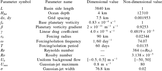
Table summarising the parameter space used in the shallow-water simulations. Both dimensional and non-dimensional values are given when applicable. In some experiments, the magnitude of a uniform background flow is varied, so the entire range in which the parameter is varied is given. Values are given to four significant figures.

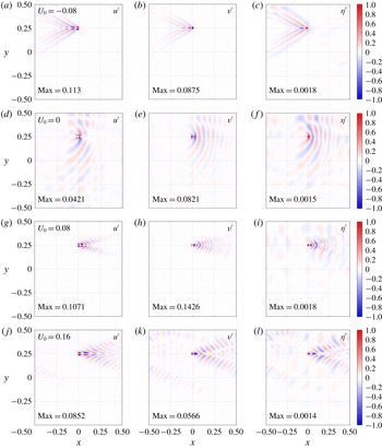
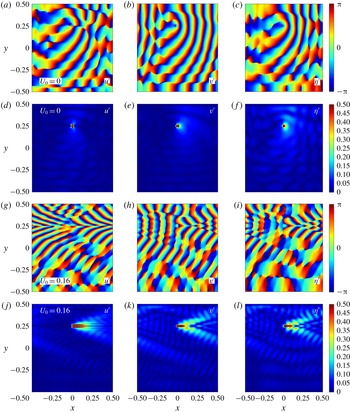
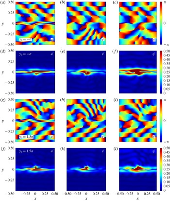
Plotted in figure 1 are snapshots of the periodic solutions, with forcing in the northern half of the domain and a selection of uniform background flows. In figure 2 are snapshots of complex amplitude and phase corresponding to a selection of the solutions in figure 1. The phase maps of the solutions exhibit wave reflection at the north–south boundaries, as well as a meridional discontinuity in the zonal velocity phase at the forcing latitude. The flow response is strongest in the vicinity of the forcing, where its spatial structure is representative of the corresponding forcing term. Over time, the forcing disturbance is radiated away and also advected by the background flow, while simultaneously spreading meridionally. For a stronger background flow, this meridional spreading is reduced, and the solution becomes meridionally confined for sufficiently strong uniform background flows. The primary effect of increasing/decreasing the frequency (in the test range
 $\unicode[STIX]{x1D714}\in [1/80,1/40]~\text{days}^{-1}$
) is the shortening/lengthening of waves in the zonal direction; due to the purely zonal background flow, the meridional structure of the solutions remains constrained by the north–south boundaries and the forcing radius. Under variations in the forcing radius, the solutions again remain qualitatively similar, with the primary effect being increased meridional spreading with increased forcing radius.
Solutions to the single-layer shallow-water system, linearised about a uniform zonal background flow and forcing in the northern half of the domain. Each row corresponds to a solution produced using a different uniform
 $U_{0}$
; the dimensional value (units
 $\text{m}~\text{s}^{-1}$
) is given the left-hand panels. Plotted is the zonal velocity perturbation (a,d,g,j), meridional velocity perturbation (b,e,h,k), SSH perturbation (c,f,i,l). Each solution component has been normalised by its maximum absolute value, as attained by non-dimensional forcing of amplitude unity. The value by which each solution component has been normalised is given in the bottom left corner in each panel. Animations show that away from the vicinity of the forcing there is large-scale westward Rossby wave propagation with phase speed
 ${\sim}0.1$
(
 $\text{m}~\text{s}^{-1}$
).

Plots of phase (a–c and g–i) and complex amplitude (d–f and j–l) corresponding to uniform background flows
 $U_{0}\in \{0.0,0.16\}~\text{m}~\text{s}^{-1}$
(indicated in a,d,g,j). The rows are arranged in pairs such that the phase and complex amplitude of the solutions are more easily viewed together. The zonal velocity is in (a,d,g,j), the meridional velocity is in (b,e,h,k), and the SSH perturbation is in (c,f,i,l). Note that the phases are cyclic data such that a phase of
 $\unicode[STIX]{x03C0}$
is equivalent to a phase of
 $-\unicode[STIX]{x03C0}$
. The amplitude colour bar is maximised at 0.5 (rather than 1) so as to better represent the amplitude in the far field.

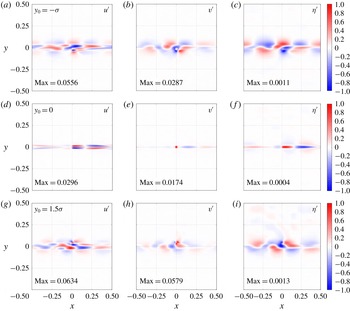
Typical solutions to the single-layer shallow-water system, linearised about a zonal Gaussian-jet background flow. Each row corresponds to a solution produced using a different forcing latitude
 $y_{0}$
, indicated in the left-hand panel of each row, relative to the axis of the jet at
 $y=0$
. Plotted is the zonal velocity perturbation (a,d,g), meridional velocity perturbation (b,e,h), SSH perturbation (c,f,i). Further details are the same as in figure 1.

Figure 3 contains solution snapshots produced with the Gaussian-jet background state defined in (2.19) and (2.20) with
 $a$
selected so that the maximum speed of the jet is
 $0.8~\text{m}~\text{s}^{-1}$
and with jet width
 $\unicode[STIX]{x1D70E}=L/50~\text{km}$
. These choices are motivated by the barotropic component of the eastward jet simulated in three-layer wind-driven double-gyre shallow-water dynamics (not shown) produced using the GOLD ocean model (Hallberg & Gnanadesikan Reference Hallberg and Gnanadesikan2006). Figure 4 displays plots of complex amplitude and phase corresponding to a selection of the solutions in figure 3. Throughout these figures, the background flow is fixed, whereas the forcing latitude
 $y_{0}\in \{-\unicode[STIX]{x1D70E},0,3\unicode[STIX]{x1D70E}/2\}$
is varied. When the forcing is located far enough away from the jet, the solution behaves very much like the zero background-flow case since locally
 $U_{0}\approx 0$
. For a central forcing the perturbation is meridionally confined and advected eastwards by the jet.
Plots of phase (a–c and g–i) and complex amplitude (d–f and j–l) with a Gaussian background flow and different choices of forcing latitude,
 $y_{0}$
(indicated in a,d,g,j). The zonal velocity is in (a,d,g,j), the meridional velocity is in (b,e,h,k) and the SSH perturbation is in (c,f,i,l). Other details are the same as in figure 2.

Forcing on the flanks of the jet induces a much more varied response. For example, varying
 $r_{0}$
in the range [60, 90] km induces solutions which are qualitatively and quantitatively similar, but for larger
 $r_{0}$
(approximately greater than 110 km), solutions become qualitatively dissimilar, with the elimination of the regular alternating eddy pattern. Varying
 $\unicode[STIX]{x1D714}$
(in the range
 $[1/80,1/40]~\text{days}^{-1}$
) induces only slight qualitative variations in the solutions, indicating that the forcing and background flow parameters are more dominant in determining the flow response. Shifting both the jet and forcing location meridionally has almost no effect on the solution pattern or its amplitude.
3 Redistribution of potential vorticity
In this section we look at the potential vorticity (PV) in the shallow-water system and consider how it is redistributed by the plunger forcing.
3.1 Defining potential vorticity
The full PV,
 $q$
, in the system is defined by
 $$\begin{eqnarray}q=\frac{\unicode[STIX]{x1D701}+{\displaystyle \frac{1}{Ro}}f}{\unicode[STIX]{x1D702}},\quad \text{where}\;\unicode[STIX]{x1D701}=\frac{\unicode[STIX]{x2202}v}{\unicode[STIX]{x2202}x}-\frac{\unicode[STIX]{x2202}u}{\unicode[STIX]{x2202}y}\end{eqnarray}$$
is the relative vorticity. Note the factor of
 $1/Ro$
multiplying the Coriolis parameter, due to the non-dimensionalisation. We define the PV anomaly induced by the forcing as
 $$\begin{eqnarray}q^{\prime }=q-Q\quad \text{where}\;Q=\frac{1}{H_{0}}\left(\frac{1}{Ro}f-\frac{\text{d}U_{0}}{\text{d}y}\right)\end{eqnarray}$$
is the background PV. See appendix B for the derivation of a PV conservation equation consistent with governing equations (2.7)–(2.9).
3.2 Potential vorticity redistribution – footprints
To begin to evaluate how PV is redistributed in the system, we define the PV footprint,
 $P$
, as the time-mean (denoted by an overbar) PV flux convergence:
 $$\begin{eqnarray}P=-\unicode[STIX]{x1D735}\boldsymbol{\cdot }(\overline{\boldsymbol{u}q}).\end{eqnarray}$$
Here,
 $\boldsymbol{u}=(u,v)$
is the horizontal velocity vector and
 $q$
is the nonlinear PV. Note that here we are assuming a quasi-linear framework, i.e. we deduce nonlinear footprints from linear solutions. The quasi-linear framework has been successfully adopted in previous studies as an approximation to the fully nonlinear case (e.g. Berloff & Kamenkovich Reference Berloff and Kamenkovich2013a
,Reference Berloff and Kamenkovich
b
; Berloff Reference Berloff2015). To calculate fully nonlinear shallow-water footprints and compare them with their quasi-linear counterparts would be an interesting research extension, but is beyond the scope of the present study. All footprints are calculated using solutions which have been normalised by the forcing amplitude.
Consider the various terms in
 $P$
:
 $$\begin{eqnarray}P=-\!\left[\frac{\unicode[STIX]{x2202}}{\unicode[STIX]{x2202}x}(\overline{u^{\prime }q^{\prime }})+\frac{\unicode[STIX]{x2202}}{\unicode[STIX]{x2202}x}(\overline{U_{0}q^{\prime }})+\frac{\unicode[STIX]{x2202}}{\unicode[STIX]{x2202}x}(\overline{u^{\prime }Q})+\frac{\unicode[STIX]{x2202}}{\unicode[STIX]{x2202}y}(\overline{v^{\prime }q^{\prime }})+\frac{\unicode[STIX]{x2202}}{\unicode[STIX]{x2202}y}(\overline{v^{\prime }Q})\right].\end{eqnarray}$$
The assumed time dependence of the solution means that the
 $u^{\prime }Q$
and
 $v^{\prime }Q$
fluxes average to zero;
 $U_{0}q^{\prime }$
has a non-zero time average due to the nonlinearity of
 $q^{\prime }$
(i.e. due to the division by
 $\unicode[STIX]{x1D702}=H_{0}+\unicode[STIX]{x1D702}^{\prime }$
in (3.1)), but its contribution to
 $P$
remains several orders of magnitude smaller than the contributions of zonal eddy PV flux (
 $u^{\prime }q^{\prime }$
) and meridional eddy PV flux (
 $v^{\prime }q^{\prime }$
) terms. With a zonally periodic system, it is useful to consider the zonal average of the footprint,
 $\langle P\rangle$
, which gives a measure of the average PV flux convergence at every latitude. Note that the zonal averaging operation means that the meridional eddy PV flux provides the only contribution to
 $\langle P\rangle$
.
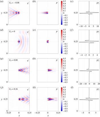
Figure 5 contains plots of the PV anomaly
 $q^{\prime }$
, the footprint
 $P$
and the footprint’s zonal average
 $\langle P\rangle$
corresponding to the uniform-flow solutions presented in the previous section. For all uniform background flows considered, the footprint is characterised by a pool of positive/negative PV flux convergence to the north/south of the forcing location, consistent with the PV structure in double-gyre circulation around the eastward jet extension of a western boundary current (Waterman & Jayne Reference Waterman and Jayne2012). This property of the footprint is a well-known result and may be explained by considering zonal momentum conservation (Haidvogel & Rhines Reference Haidvogel and Rhines1983; Waterman & Jayne Reference Waterman and Jayne2012). Away from the forced latitudes we have large-scale westward Rossby wave and westward momentum propagation. Zonal momentum conservation therefore requires a convergence of eastward momentum at the forced latitudes, which itself corresponds to a northward convergence of PV flux. This conclusion may also be reached by considering the shape of ‘eddies’ which propagate away from the forcing location. The anisotropic ‘bow-shaped’ eddies, most easily observable in plots of
 $\unicode[STIX]{x1D702}^{\prime }$
for weaker
 $U_{0}$
, are responsible for a northward flux of zonal momentum (
 $u^{\prime }v^{\prime }>0$
) south of
 $y_{0}$
and a southward flux (
 $u^{\prime }v^{\prime }<0$
) north of
 $y_{0}$
(see Wardle & Marshall (Reference Wardle and Marshall2000), figure 5, for a clear diagram depicting this phenomenon). This leads to a convergence of eastward momentum at the forced latitudes, and thus PV flux convergence to the north of
 $y_{0}$
.
Potential vorticity anomaly (a,d,g,j), footprint (b,e,h,k) and footprint zonal average (c,f,i,l) corresponding to the uniform background-flow solutions presented in figure 1. The dimensional value of the zonal background flow (units
 $\text{m}~\text{s}^{-1}$
) is given in the left-hand panel of each row. PV and footprints are calculated using solutions which have been normalised by the forcing amplitude, from which the zonal average of the footprint is calculated. The PV and the footprint are re-normalised so that their maximum absolute values are 1. For optimum presentation, the colour bar range is
 $[-0.5,0.5]$
, and the plots are ‘zoomed in’ on the forcing region. The footprint zonal averages have been scaled up by a factor of
 $10^{5}$
.

Fully nonlinear quasi-geostrophic PV footprints are presented in Waterman & Jayne (Reference Waterman and Jayne2012), and meridional slices of
 $P$
are presented in Haidvogel & Rhines (Reference Haidvogel and Rhines1983). In both these studies, the footprint exhibits a similar dipole structure to those presented in this study, thus confirming the capability of the quasi-linear framework as an approximation to the nonlinear case. In the multi-layer quasi-geostrophic system, the (quasi-linear) footprint dipole structure is negated for westward background flows (Berloff Reference Berloff2015), and it is hypothesised that the same would occur in the multi-layer shallow-water system once baroclinicity is introduced, but this extension is left for a later study.
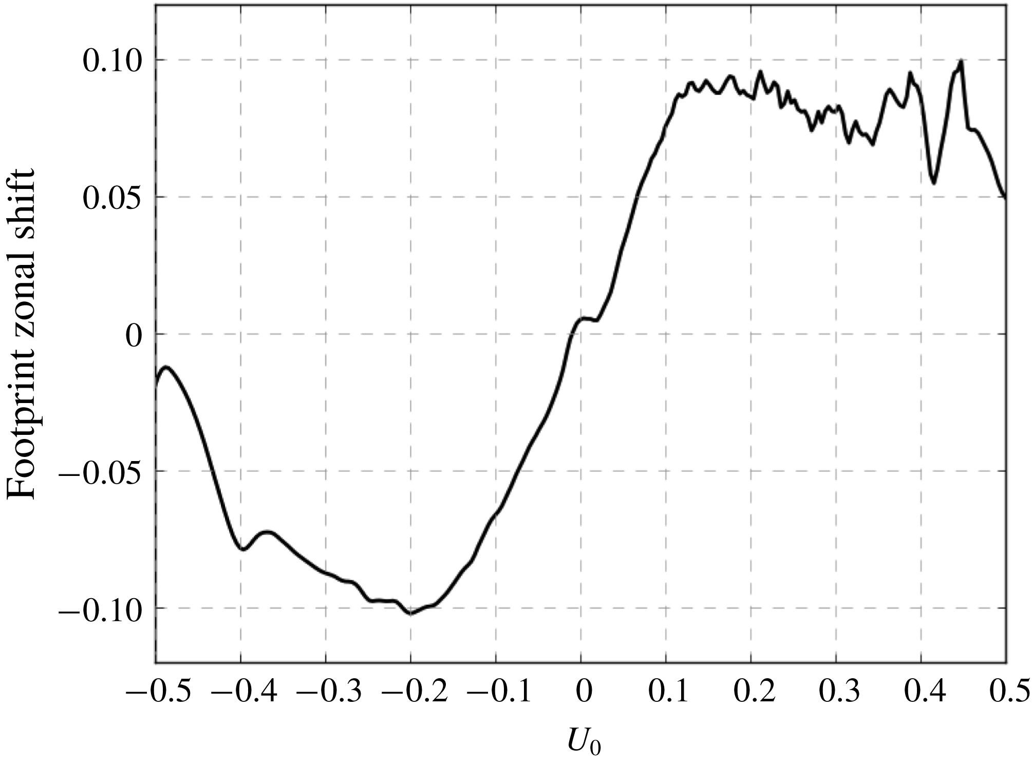
Dependent on the direction and magnitude of the background flow, the dipole structure of the footprint is shifted zonally, with initial observations indicating that the footprint response is concentrated downstream of the background flow. We can quantify this more precisely by defining a zonal ‘centre of mass’, namely
 $x_{shift}$
, of the footprint:
 $$\begin{eqnarray}x_{shift}=\frac{\displaystyle \int _{-1/2}^{1/2}x\hat{P}\,\text{d}x}{\displaystyle \int _{-1/2}^{1/2}\hat{P}\,\text{d}x}\quad \text{where}\;\hat{P}=\int _{-1/2}^{1/2}|P|\,\text{d}y.\end{eqnarray}$$
The zonal shift is plotted against the uniform background flow
 $U_{0}\in [-0.5,0.5]~\text{m}~\text{s}^{-1}$
in figure 6. Excluding weak
 $U_{0}\approx 0$
, the footprint shift is in the same direction of
 $U_{0}$
due to the advection of the forcing disturbance by the background flow. The maximum shift,
 $|x_{shift}|\approx 0.1$
, corresponds to a dimensional footprint shift of approximately 400 km. With such large values, it is argued that the downstream shift of the footprint should be accounted for in parameterisations of eddy fluxes. For large
 $|U_{0}|$
, the zonal shift becomes saturated, which is possibly due to the unavailability of eigenmodes with sufficiently large phase speeds.
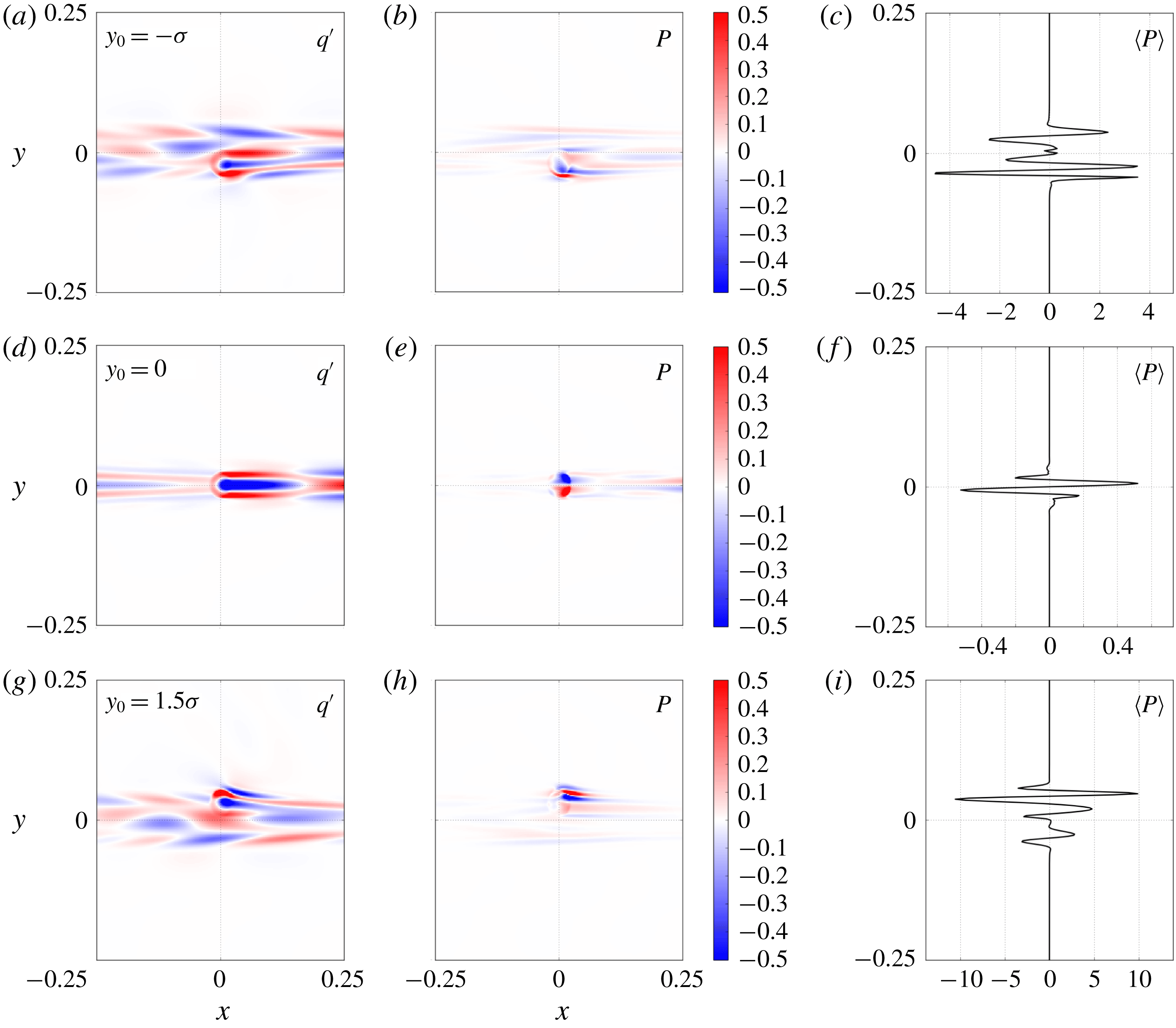
The PV anomalies, footprints and footprint zonal averages corresponding to the Gaussian-jet solutions in the previous section are presented in figure 7. The footprints, specifically the zonal averages, indicate that in the presence of a zonal jet the plunger does not efficiently redistribute positive/negative PV to the north/south as was the case with the uniform background flows. Moreover, when forcing on the flanks of the background jet, net-northward or net-southward PV flux convergences are possible, which correspond to a sharpening or broadening of the jet profile, respectively. The behaviour of the footprints in both background-flow cases motivates the definition of a more succinct measure of the PV redistribution, namely the equivalent eddy flux, discussed in the next subsection.
Zonal shift (dimensionless) of the centre of mass of the footprint plotted against uniform
 $U_{0}$
given in units
 $\text{m}~\text{s}^{-1}$
. In dimensional units, the maximum zonal shifts are of the order of 400 km.

Potential vorticity anomaly (a,d,g), footprint (b,e,h) and footprint zonal average (c,f,i) corresponding to the Gaussian-jet background flow solutions presented in figure 3. The forcing latitude
 $y_{0}$
is indicated in (a,d,g). All other details are identical to those given in the caption of figure 5.

3.3 Equivalent eddy fluxes
Here we define the equivalent eddy flux (EEF) as the net PV flux convergence to the north of a reference latitude
 $y_{0}^{\prime }$
, multiplied by a redistribution length scale, minus the same value evaluated south of
 $y_{0}^{\prime }$
. The northern component is
 $$\begin{eqnarray}{\mathcal{P}}_{N}\equiv L_{N}\int _{y>y_{0}^{\prime }}\langle P\rangle \,\text{d}y\quad \text{where}\;L_{N}=\frac{\displaystyle \int _{y>y_{0}^{\prime }}|y-y_{0}^{\prime }|\,|\langle P\rangle |\,\text{d}y}{\displaystyle \int _{y>y_{0}^{\prime }}|\langle P\rangle |\,\text{d}y}.\end{eqnarray}$$
The equivalent southern quantities
 ${\mathcal{P}}_{S}$
and
 $L_{S}$
are defined with
 $y<y_{0}^{\prime }$
in the integration limits, so that we may define the EEF as follows:
 $$\begin{eqnarray}{\mathcal{P}}\equiv {\mathcal{P}}_{N}-{\mathcal{P}}_{S}.\end{eqnarray}$$
We define the reference latitude as
 $y_{0}^{\prime }$
as the ‘centre of PV redistribution’, namely, the centre of mass of
 $|\langle P\rangle |$
:
 $$\begin{eqnarray}y_{0}^{\prime }=\frac{\displaystyle \int _{-1/2}^{1/2}y|\langle P\rangle |\,\text{d}y}{\displaystyle \int _{-1/2}^{1/2}|\langle P\rangle |\,\text{d}y}.\end{eqnarray}$$
For uniform background flows the reference latitude is the same as the forcing latitude, i.e.
 $y_{0}^{\prime }=y_{0}$
. When forcing on the flanks of Gaussian-jet background flow, however, the centre of PV redistribution is typically skewed towards the jet core.
To motivate the definition of the EEF (3.6, 3.7), consider the footprint’s dipole structure as in figure 5, in which case the length scales (
 $L_{N},L_{S}$
) may be interpreted as a measure of the ‘distance’ between the pools of positive/negative PV flux convergence. If the two pools are located far away from one another, then this corresponds to a larger extent of PV redistribution, and is quantified by relatively large length scales. Conversely, if the two pools are located close to one another, the length scales would be smaller since PV has been redistributed over a shorter distance.
The EEF is a simple scalar measure of the extent of the meridional PV redistribution, provided in terms of the footprint. Its simplicity is indeed part of the motivation for defining it, with the intention that it provides a useful measure of the properties of the more complicated footprint (which is a two-dimensional scalar field). In Berloff (Reference Berloff2015, Reference Berloff2016) the EEF is used as a basis for a parameterisation of eddy PV fluxes by providing a scaling factor for dipole inputs of PV in a non-eddy-resolving model. Subsequent simulations on the coarse-resolution grid exhibit a coherent eastward jet, which is otherwise absent in such a low-resolution model. We focus on the EEF’s dependence on: (i) the magnitude and direction of a uniform background flow
 $U_{0}$
, (ii) the magnitude and width of a Gaussian-jet background flow and (iii) the forcing latitude
 $y_{0}$
for both uniform and Gaussian-jet background flows.
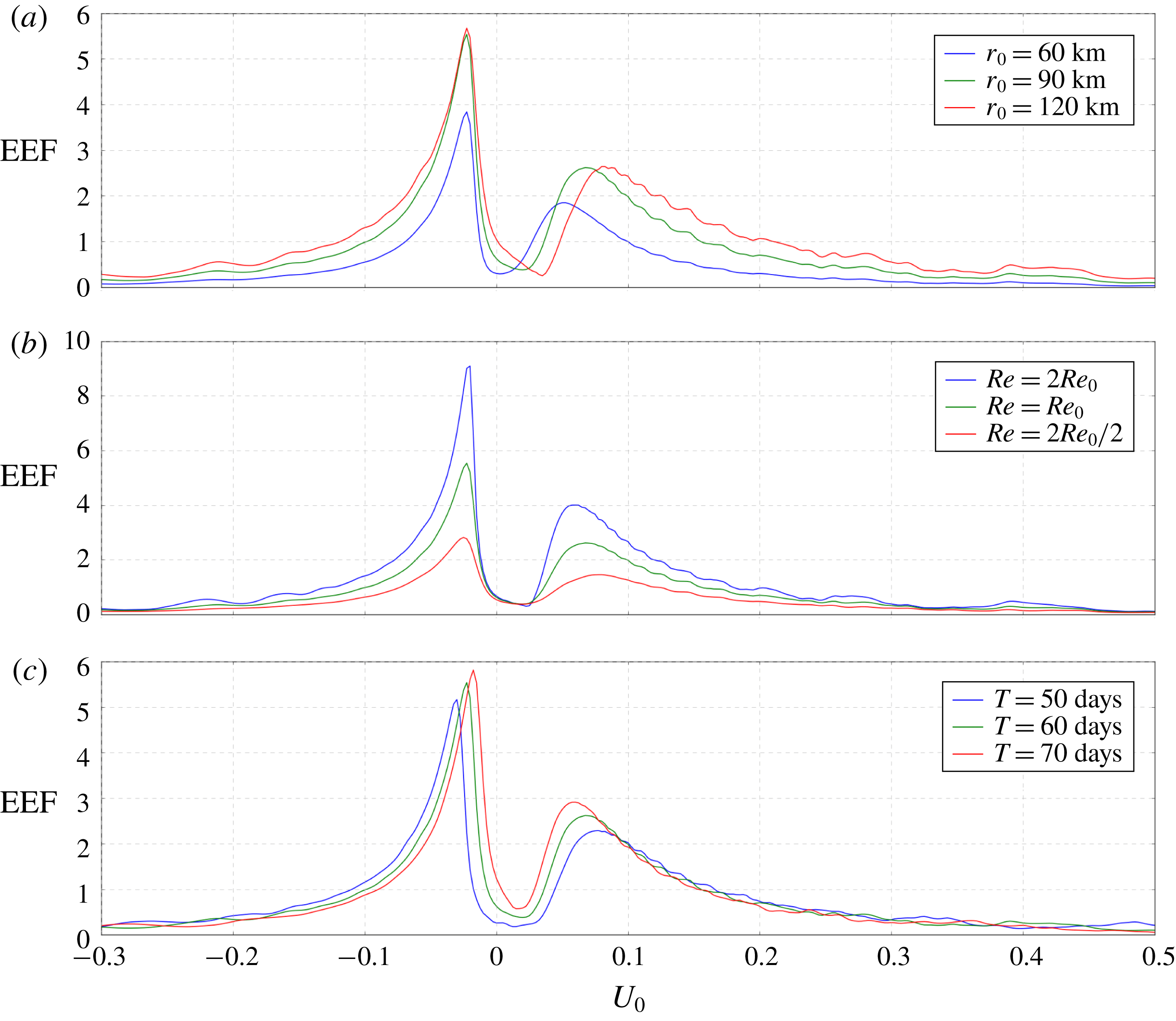
Plots of the EEF versus uniform background flow
 $U_{0}\in [-0.3,0.5]~\text{m}~\text{s}^{-1}$
are shown in figure 8. The effects of varying three other parameters are considered: (i) the forcing radius,
 $r_{0}$
, (ii) the Reynolds number,
 $Re$
, and (iii) the forcing period,
 $T=1/\unicode[STIX]{x1D714}$
. First of all, the EEF is positive for all
 $U_{0}\in [-0.3,0.5]$
, and for all parameters considered, so that in the presence of uniform background flow the plunger forcing induces a net-northward flux of PV. In the multi-layer shallow-water system, we might instead expect net-negative upper-layer PV flux convergence for uniform westward background flows; confirmation of this is left to a later study, but is indeed the case in the multi-layer quasi-geostrophic system (Berloff Reference Berloff2015).
Plots of the equivalent eddy flux versus uniform background flow
 $U_{0}$
for a range of parameter values. From (a) to (c), parameters varied in each plot are the forcing radius (
 $r_{0}$
), the Reynolds number (
 $Re$
) and the forcing period (
 $T=1/\unicode[STIX]{x1D714}$
). Note that the vertical axis scale differs in each plot, and that the green line, representing the reference parameter selection, is the same in each plot. All EEFs have been scaled up by a factor of
 $10^{7}$
.

The EEF robustly has two local maxima, one for eastward background flow at
 $U_{0}=U_{e}$
, say, and a larger one for westward background flow at
 $U_{0}=U_{w}$
. In between, we have a local minimum for weak eastward flow at
 $U_{0}=U_{min}$
. As
 $|U_{0}|$
grows large, the EEF decays to a small positive value. We can begin to understand EEF profile by considering eigenmode decompositions of solutions. When
 $U_{0}=U_{w}$
or
 $U_{0}=U_{e}$
, a wide range of eigenmodes are excited, each with relatively large amplitude, resulting in particularly strong flow responses and therefore large PV redistribution. As the magnitude of the background flow continues to grow larger, a progressively smaller set of eigenmodes are excited, resulting in the gradual weakening of the EEF for large
 $|U_{0}|$
. For a background flow
 $U_{0}=U_{min}$
, there is no notable excitation of any eigenmodes, and we observe a correspondingly weak EEF. A second contributor to the EEF’s behaviour is the extent of the interaction between zonal and meridional momentum-flow components. The magnitude and direction of
 $U_{0}$
dictates the shape and propagation of the forcing disturbance, and we find that the minimum in the EEF coincides with the
 $U_{0}$
-value at which the forcing disturbance does not propagate. With no propagation, the ‘eddies’ have zonal and meridional momentum components that remain entirely out of phase with each other, and therefore their interaction is minimised, resulting in minimal EEF values. This lack of interaction may be confirmed by considering the correlation between zonal and meridional momentum components, but an in-depth analysis in this vein is left for a later study.
The maxima of the EEF are extremely sensitive to
 $Re$
in the explored range of values, and we ran individual simulations to test this sensitivity further. With the background flow fixed at
 $U_{0}=U_{w}$
, we gradually increase
 $Re$
through the range
 $[2Re_{0},10Re_{0}]$
, and find that the EEF initially continues to grow larger but quickly becomes weakly insensitive to further adjustments to
 $Re$
. It is argued that this saturation is physical rather than being due to grid resolution limitations. Another notable property of the EEF is the shift of the maxima toward larger
 $|U_{0}|$
as the forcing period shortens, which can be explained by the (inviscid) Rossby wave dispersion relation:
 $$\begin{eqnarray}\unicode[STIX]{x1D714}=U_{0}k-\frac{\unicode[STIX]{x1D6FD}k}{k^{2}+l^{2}},\end{eqnarray}$$
where
 $k$
and
 $l$
are the zonal and meridional wavenumbers, respectively. Excited wavenumbers
 $k$
have the same sign as
 $U_{0}$
, so that
 $U_{0}k>0$
. Therefore, if we shorten the forcing/solution period, i.e. increase
 $\unicode[STIX]{x1D714}$
, then the available modes shift toward larger
 $k$
, or the same
 $k$
modes become available at larger
 $U_{0}$
.
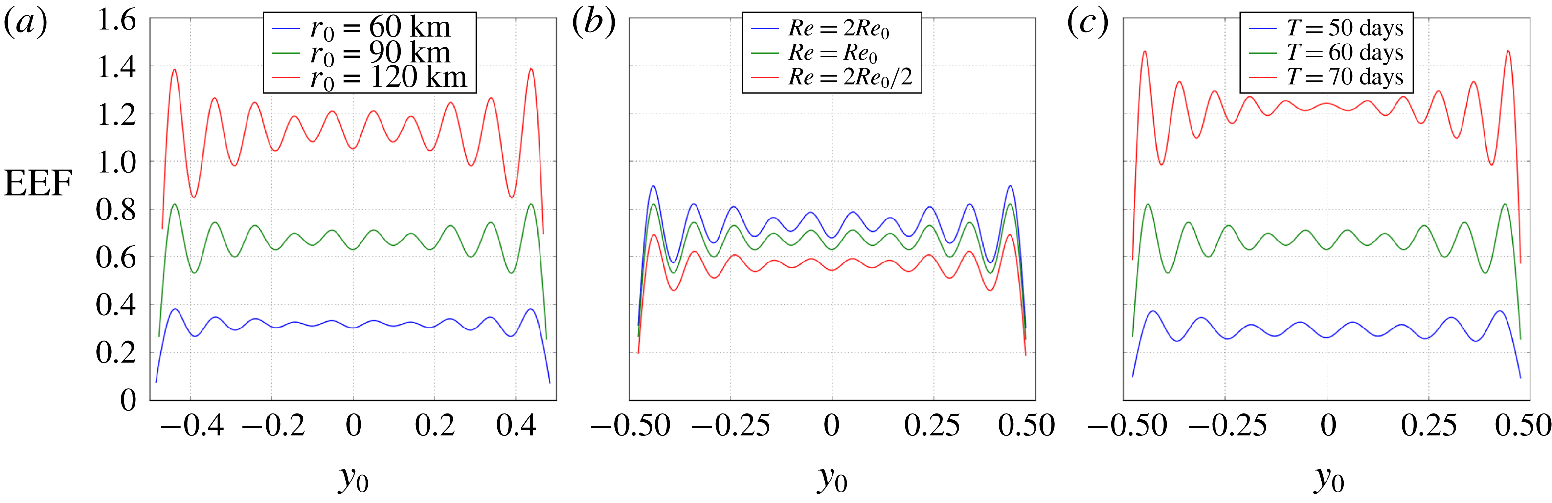
Plotted in figure 9 is the equivalent eddy flux versus forcing latitude,
 $y_{0}$
, for a selection of
 $r_{0}$
,
 $Re$
and
 $T$
, with zero background flow fixed throughout. The presence of the northern/southern boundaries in the system causes the EEF to oscillate as
 $y_{0}$
is varied. These oscillations grow larger near the boundaries, but the EEF remains positive so that we retain the net-northward convergence of PV flux domainwide. For non-zero uniform background flows, the oscillations in the EEF are suppressed depending on the availability of channel modes for that particular
 $U_{0}$
.
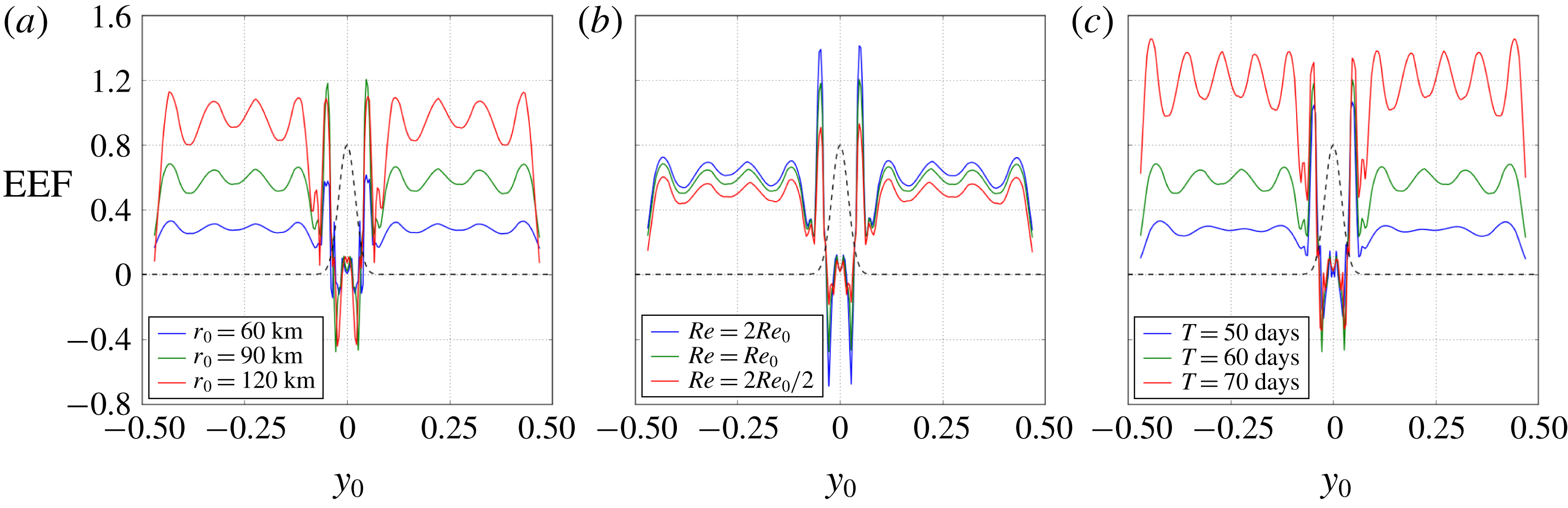
In figure 10 plots of the EEF versus
 $y_{0}$
with the reference Gaussian-jet background flow are displayed. Away from the (central) jet region, the EEF closely resembles the corresponding EEF curves for
 $U_{0}=0$
in figure 9, whereas in the jet region the EEF profile is more complicated. In this jet region we interpret a positive EEF as a net sharpening of the jet, attained via eastward acceleration of the jet core and westward acceleration (recirculation) of the jet flanks. On the other hand, a negative EEF corresponds to a net broadening of the jet profile, attained by deceleration of the jet core and eastward acceleration of the jet flanks. Here we reiterate that the EEF and its interpretations are purely diagnostic, as they are formulated in the quasi-linear approximation with no feedback into the dynamics of the shallow-water model in this study. For forcing located on the outer jet flanks (
 $|y_{0}|\in [0.03,0.05]$
), typical flow response is dominated by waves with short zonal wavelengths whose meridional propagation towards the jet core is inhibited by turning lines (O’Rourke & Vallis Reference O’Rourke and Vallis2013, Reference O’Rourke and Vallis2016). This results in localised nonlinear self-interaction and positive EEFs via a similar mechanism as in the uniform background-flow case. On the inner jet flanks (
 $|y_{0}|\in [0.01,0.03]$
), plunger interaction with the jet core induces zonally large-scale waves (
 $|k|\leqslant 4$
) that straddle the jet core. As in O’Rourke & Vallis (Reference O’Rourke and Vallis2013, Reference O’Rourke and Vallis2016), the nonlinear self-interaction of these waves acts to decelerate the jet core and accelerate the flanks, thus broadening the jet profile, quantified by a negative EEF. Forcing centred on the jet core (
 $y_{0}\in [-0.01,0.01]$
) induces a small positive EEF.
Plots of the equivalent eddy flux against plunger forcing latitude,
 $y_{0}$
, for various values of forcing radius (a), Reynolds number (b) and forcing period (c). The shallow-water system has been linearised about a zero background flow. The green line in each plot corresponds to the reference parameter set-up. All EEFs have been scaled up by a factor of
 $10^{7}$
.

Plots of the equivalent eddy flux against plunger forcing latitude,
 $y_{0}$
, for various values of forcing radius (a), Reynolds number (b) and forcing period (c). Here the shallow-water governing equations are linearised about the reference Gaussian-jet background flow (black dashed line). Other details are the same as in figure 9.

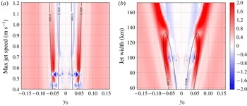
We also experiment with the maximum jet speed and jet width, varying one at a time. Figure 11 displays the EEF plotted against forcing latitude (central third of the domain only) and either maximum Gaussian-jet speed (left) or jet width (right). The behaviour described in the above paragraph persists for all jet widths considered (
 $\unicode[STIX]{x1D70E}\in [0.015L,0.045L]~\text{km}$
), and for maximum jet speeds in the range
 $U_{max}\in [0.6,1.2]~\text{m}~\text{s}^{-1}$
. However, for weak jets such that
 $U_{max}\in [0.4,0.6]~\text{m}~\text{s}^{-1}$
(left-hand plot) this scenario breaks down as we have negative EEF values on the outer jet flanks. Here the plunger forcing does not interact directly with the jet core, but nonetheless excites large-scale zonal waves that propagate into the jet core, uninhibited by turning lines. Again these large-scale waves decelerate the core of the background jet, and accelerate the flanks.
Equivalent eddy flux against plunger-forcing latitude
 $y_{0}$
, and either maximum jet speed (a) or jet width (b). The jet width and the maximum jet speed are fixed at their reference values in the left and right plots, respectively. In each plot, the black contours correspond to zero background PV gradient, outlining two lobes inside of which the background PV gradient is negative. Forcing latitudes are limited to the central third of the domain. All other parameters are as in the reference set-up (table 1). EEFs are scaled up by
 $10^{7}$
.

To summarise the main results of this section, we find that the plunger forcing induces a northward PV flux convergence for uniform zonal background flows. The extent of this redistribution, quantified by the EEF (figure 8), has a maximum for weak westward flow and a secondary maximum for eastward flow. With robust dependence on uniform
 $U_{0}$
, the EEF can be used to provide a basis for a parameterisation of eddy PV fluxes, as has been done in the quasi-geostrophic system (Berloff Reference Berloff2015, Reference Berloff2016). Plunger forcing on the outer flanks of a Gaussian jet acts to sharpen the jet profile, whereas a plunger forcing closer to the jet core, such that there is direct interaction with the jet core, is likely to broaden the jet profile.
4 Extension to stochastic forcing
In this section we extend the shallow-water system used in this study to account for external forcing with stochastic time dependence,
 $S(t)$
, so that
 $F_{i}(x,y,t)=F_{i}(x,y)S(t)$
,
 $i=1,2,3$
. Fourier transforming equations (2.7)–(2.9) in time (as well as
 $x$
), yields governing equations similar to (2.11)–(2.13):
 $$\begin{eqnarray}\displaystyle & \displaystyle \left[\text{i}\unicode[STIX]{x1D6FF}Ro+4\unicode[STIX]{x03C0}^{2}k^{2}\frac{Ro}{Re}+\unicode[STIX]{x1D6FE}\right]\tilde{u} -\frac{Ro}{Re}\frac{\unicode[STIX]{x2202}^{2}\tilde{u} }{\unicode[STIX]{x2202}y^{2}}+\left[Ro\frac{\text{d}U_{0}}{\text{d}y}-f\right]\tilde{v}+2\unicode[STIX]{x03C0}\text{i}k\tilde{\unicode[STIX]{x1D702}}=\tilde{S}(w)\tilde{F}_{1}, & \displaystyle\end{eqnarray}$$
 $$\begin{eqnarray}\displaystyle & \displaystyle \left[\text{i}\unicode[STIX]{x1D6FF}Ro+4\unicode[STIX]{x03C0}^{2}k^{2}\frac{Ro}{Re}+\unicode[STIX]{x1D6FE}\right]\tilde{v}-\frac{Ro}{Re}\frac{\unicode[STIX]{x2202}^{2}\tilde{v}}{\unicode[STIX]{x2202}y^{2}}+f\tilde{u} +\frac{\unicode[STIX]{x2202}\tilde{\unicode[STIX]{x1D702}}}{\unicode[STIX]{x2202}y}=\tilde{S}(w)\tilde{F}_{2}, & \displaystyle\end{eqnarray}$$
 $$\begin{eqnarray}\displaystyle & \displaystyle \text{i}\unicode[STIX]{x1D6FF}\tilde{\unicode[STIX]{x1D702}}+2\unicode[STIX]{x03C0}\text{i}kH_{0}\tilde{u} +\frac{\text{d}H_{0}}{\text{d}y}\tilde{v}+H_{0}\frac{\unicode[STIX]{x2202}\tilde{v}}{\unicode[STIX]{x2202}y}=\tilde{S}(w)\tilde{F}_{3}, & \displaystyle\end{eqnarray}$$
where
 $\tilde{u} \equiv \tilde{u} (k;y;\unicode[STIX]{x1D714})$
is the Fourier transform in
 $x$
and
 $t$
of
 $u^{\prime }$
, and
 $\unicode[STIX]{x1D6FF}(k;y;\unicode[STIX]{x1D714})=2\unicode[STIX]{x03C0}(U_{0}k+\unicode[STIX]{x1D714})$
. Stochastically forced solutions may then be obtained by implementing the algorithm detailed in § 2.2 for a spectrum of forcing frequencies,
 $\unicode[STIX]{x1D6FA}$
, say.
As an example, we model the time dependence as a Gaussian process,
 $S^{\ast }(t)$
, multiplied by a Planck-taper window,
 $w(t)$
, to impose that
 $S(t)=S^{\ast }(t)w(t)=0$
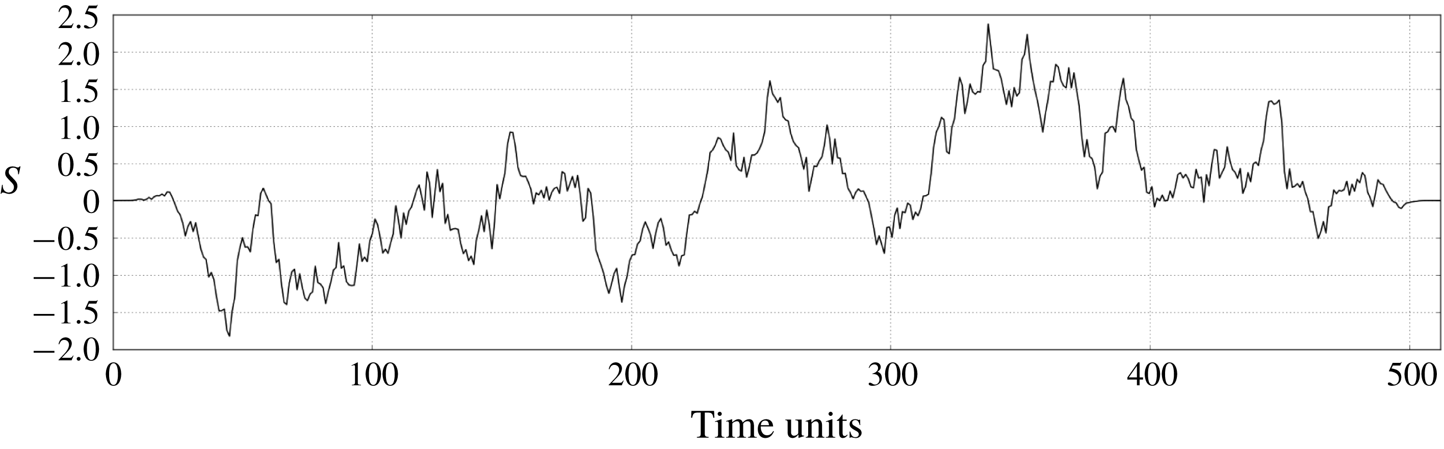
at the beginning and end of the forcing interval. This stochastic process, shown in figure 12, is modelled over
 $512$
time samples and has exponentially decaying autocorrelation with characteristic time scale
 $\unicode[STIX]{x1D70F}=50$
time units. The spatial dependence of
 $F_{i}$
remains the same as defined in § 2.3.
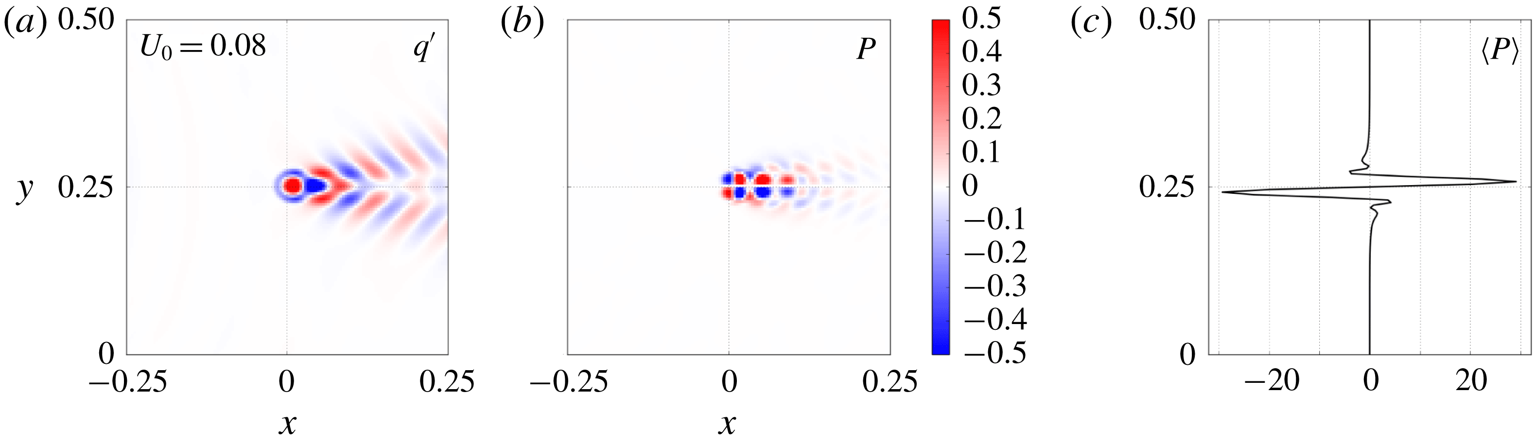
Figure 13 contains plots of PV redistribution diagnostics corresponding to the stochastically forced solutions with uniform background flow,
 $U_{0}=0.08~\text{m}~\text{s}^{-1}$
. The flow response (not shown) and the PV anomaly are extremely similar to the case of periodic time dependence (figure 1), but the PV footprint is noticeably different. The footprint now has a multiple dipoles aligned zonally, due to modes of varying frequency interacting with each other. Nonetheless, the zonally averaged footprint retains much the same properties as in the case of periodic forcing.
An example Gaussian process, multiplied by a Planck-taper window to ensure zero values at the beginning and end of the forcing interval. The time series has 512 time samples with a decorrelation time scale
 $\unicode[STIX]{x1D70F}=50$
time units.

PV snapshot (a), footprint (b) and zonally averaged footprint (c) corresponding to the stochastically forced solutions. Other details are the same as in figure 5.

5 Summary and applications
Since simulations of eddy-resolving models are often computationally unfeasible, a parameterisation of eddy effects on the large-scale flow is required. Defining such a parameterisation via understanding of potential vorticity (PV) fluxes is one of numerous avenues for accounting for the effects of turbulent eddies in a non-eddy-resolving ocean model. Most commonly implemented in general circulation models (GCMs) is the parameterisation of Gent & McWilliams (Reference Gent and McWilliams1990) which assumes that eddies act to flux tracers down their large-scale gradient and along isopycnal surfaces. For a constant thickness diffusivity,
 $k$
, this parameterisation equates to down-gradient diffusion along isopycnals, but it is understood that
 $k$
should in fact have spatial dependence (Rypina et al.
Reference Rypina, Kamenkovich, Berloff and Pratt2012), and numerous studies have attempted to define such space-dependent
 $k$
(e.g. Killworth Reference Killworth1997; Eden Reference Eden2011; Marshall et al.
Reference Marshall, Maddison and Berloff2012; Ivchenko et al.
Reference Ivchenko, Sinha, Zalesny, Marsh and Blaker2013). Although allowing for improvements in the performance of GCMs (Danabasoglu et al.
Reference Danabasoglu, McWilliams and Gent1994), the diffusive approach naturally fails in regions of ‘anti-diffusive’ flows. For example, near eastward jets active tracers such as buoyancy, momentum and PV may be fluxed up their large-scale gradient (Starr Reference Starr1968). A stochastic parameterisation (e.g. Berloff Reference Berloff2005c
; Porta Mana & Zanna Reference Porta Mana and Zanna2014) can allow for both positive and negative eddy diffusivities, making it a more suitable method for the parameterisation of up-gradient fluxes of active tracers. The aim of such a parameterisation is to define a random-forcing term which accounts for the missing eddy effects and is closed on the large-scale flow. The present study is a logical step towards a stochastic parameterisation as it develops an understanding of flow responses to a localised, periodic plunger forcing, which is intended to represent transient eddy flux divergences.
In this study, the single-layer shallow-water system, set-up in a
 $\unicode[STIX]{x1D6FD}$
-plane channel, is linearised about a latitude-dependent zonal background flow and corresponding geostrophic sea-surface height. The plunger-induced footprint – defined in the quasi-linear framework as the time-averaged PV flux convergence – and its dependence on background-flow parameters and plunger characteristics is the primary focus. For uniform background flows, a typical footprint consists of a pool of positive/negative PV flux convergence to the north/south (poleward/equatorward) of the forcing location, which corresponds to a net-positive convergence of PV flux to the north. A similar footprint dipole structure has been observed in the fully nonlinear quasi-geostrophic system (Haidvogel & Rhines Reference Haidvogel and Rhines1983; Waterman & Jayne Reference Waterman and Jayne2012), thus promoting the capabilities of the quasi-linear approximation adopted in this study. Dependent on the uniform background flow, the dipole structure of the footprint is shifted zonally. This shift, downstream of the background flow, can be as large as 400 km, and therefore should be accounted for in a parameterisation of eddy fluxes. The footprint behaviour is more obscure for a Gaussian-jet background flow, thus motivating the definition of a more succinct measure of the meridional PV redistribution, namely, the equivalent eddy flux (EEF). The EEF is calculated by separately integrating the zonal average of the footprint to the north and south of the forcing latitude, multiplying by a length scale over which the plunger redistributes PV meridionally, and then by subtracting the southern component from the northern one. The result is a scalar value quantifying the extent of the meridional PV redistribution by the plunger forcing.
For uniform background flows, the EEF remains positive for all plunger forcing latitudes corresponding to northwards PV flux convergence. Keeping the forcing latitude fixed, the EEF has a robust bimodal structure when plotted against uniform background flow
 $U_{0}\in [-0.3,0.5]~\text{m}~\text{s}^{-1}$
(see figure 8): one maximum for weak westward background flows, one smaller maximum for eastward background flows and a minimum in between for weak eastward flow. The maxima occur for
 $U_{0}=U_{w}\in [-0.031,-0.018]~\text{m}~\text{s}^{-1}$
and
 $U_{0}=U_{e}\in [0.018,0.081]~\text{m}~\text{s}^{-1}$
, respectively (dependent on forcing radius, latitude, frequency and Reynolds number). As the uniform background flow grows larger in magnitude, the EEF tends to a small positive value. The behaviour of the EEF may be attributed to two properties of the solutions. Firstly, eigenmode decompositions indicate that a wide range of modes are excited for
 $U_{0}\approx U_{w}$
and
 $U_{0}\approx U_{e}$
, which results in relatively strong flow responses, and therefore a large EEF. Secondly, in our solutions the shape and propagation of the forcing disturbance determines the extent of interaction between eddies of zonal and meridional momentum. It is found, for example, that the minimum in the EEF coincides with the
 $U_{0}$
-value at which the forcing disturbance does not propagate. With no propagation, eddies of zonal and meridional momentum remain isotropic, and out of phase with one another. This results in a lack of interaction and minimal EEF values. These ideas are to be explored in more detail in a later study.
We also considered the PV redistribution in the presence of a Gaussian-jet background flow. We find that the proximity of the forcing to the jet core plays a crucial role in determining the nature of the PV redistribution. On the outer flanks of the jet, we generally have strong positive EEF values, corresponding to a sharpening of the jet profile which is attained by eastward acceleration of the jet core and westward acceleration of the flanks. On the inner flanks of the jet, where the forcing interacts directly with the jet core, large-scale zonal waves are excited which act to decelerate the jet core (O’Rourke & Vallis Reference O’Rourke and Vallis2013, Reference O’Rourke and Vallis2016) and broaden the jet profile. Note that all conclusions regarding EEFs are diagnostic and are a quasi-linear approximation to the nonlinear case. To compare our findings to the fully nonlinear case would be a worthwhile extension.
The footprints and EEFs provide a basis on which a future parameterisation of eddy PV fluxes can be built, and their robust dependence on background flow and forcing parameters is useful for closing a parameterisation on the large-scale flow. In the quasi-geostrophic framework, the footprints and EEFs have previously been used to define an eddy parameterisation to be included in a non-eddy-resolving model. In Berloff (Reference Berloff2015), a series of PV dipoles are scaled by the footprint and strategically placed (motivated by eddy-resolving simulations) to form an external forcing in a non-eddy-resolving model. In the resulting simulation a coherent eastward jet extension – otherwise absent in the non-eddy-resolving model – forms, thus highlighting the capabilities of the so-called plunger footprint method. It will be the aim of a future study to apply this method in the shallow-water system, and thus define an eddy parameterisation in a nonlinear shallow-water model.
In comparison to previous studies, in particular Berloff (Reference Berloff2015), the present study is novel due to its use of the
 $\unicode[STIX]{x1D6FD}$
-plane shallow-water model which is inhomogeneous with latitude, as opposed to the homogeneous quasi-geostrophic model. We also have latitude-dependent forcing terms, background velocity and background sea-surface height which provide other novel aspects. Furthermore, in Berloff (Reference Berloff2015), in which a doubly periodic domain is used, analytic methods are sufficient to calculate plunger-induced solutions, whereas here we must invoke both numerical and analytic methods in order to solve the governing equations in a singly periodic domain.
The findings of the present study highlight numerous options for further progression. (i) To consider equivalent eddy fluxes of momentum (zonal and meridional) and buoyancy would be worthwhile, since a parameterisation of eddy momentum fluxes or eddy buoyancy fluxes can be more directly included in a primitive equation model; a parameterisation of eddy PV fluxes will require a mapping of the parameterisation into prognostic variables. (ii) Extending the EEF analysis to the multi-layer shallow-water system will allow for a more comprehensive eddy parameterisation, as the effects of baroclinic instability will begin to be modelled. (iii) We have shown that the shallow-water solver used in this study can account for forcing with stochastic time dependence, but upgrading the algorithm to a time stepping method would be a worthwhile extension. (iv) To consider how the energetics of the shallow-water system depend on the forcing and background-flow parameters would be an interesting extension. For example, do the maxima of the EEF correspond to highly energetic solutions? (v) In this study we employ the quasi-linear approximation to produce PV footprints which are qualitatively similar to footprints produced in the fully nonlinear quasi-geostrophic system (Haidvogel & Rhines Reference Haidvogel and Rhines1983; Waterman & Jayne Reference Waterman and Jayne2012). A desirable extension would be to compute fully nonlinear footprints in the shallow-water system, allowing for further testing of the quasi-linear approximation.
Appendix A. Shallow-water equation non-dimensionalisation
The dimensional shallow-water equations for a single fluid layer are:
 $$\begin{eqnarray}\displaystyle & \displaystyle \frac{\text{D}u}{\text{D}t}-fv=-g\frac{\unicode[STIX]{x2202}\unicode[STIX]{x1D702}}{\unicode[STIX]{x2202}x}+\unicode[STIX]{x1D708}\unicode[STIX]{x1D6FB}^{2}u-\unicode[STIX]{x1D6FE}u+F_{1}, & \displaystyle\end{eqnarray}$$
 $$\begin{eqnarray}\displaystyle & \displaystyle \frac{\text{D}v}{\text{D}t}+fu=-g\frac{\unicode[STIX]{x2202}\unicode[STIX]{x1D702}}{\unicode[STIX]{x2202}y}+\unicode[STIX]{x1D708}\unicode[STIX]{x1D6FB}^{2}v-\unicode[STIX]{x1D6FE}v+F_{2}, & \displaystyle\end{eqnarray}$$
 $$\begin{eqnarray}\displaystyle & \displaystyle \frac{\text{D}\unicode[STIX]{x1D702}}{\text{D}t}+\unicode[STIX]{x1D702}\left(\frac{\unicode[STIX]{x2202}u}{\unicode[STIX]{x2202}x}+\frac{\unicode[STIX]{x2202}v}{\unicode[STIX]{x2202}y}\right)=F_{3}. & \displaystyle\end{eqnarray}$$
 $\unicode[STIX]{x1D708}$
and the vertical acceleration due to gravity
 $g$
. For the non-dimensionalisation, the velocity scale is
 $U=0.01~\text{m}~\text{s}^{-1}$
and the length scale is
 $L=3840~\text{km}$
, which is the basin size. The Lagrangian derivatives and forcing terms are scaled using the advective time scale,
 $T_{adv}=L/U$
, while the Coriolis parameter is scaled by itself. The ocean depth
 $\unicode[STIX]{x1D702}$
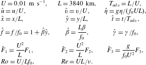
is scaled by considering geostrophic balance. Table 2 presents a summary of the dimensional scales and the dimensionless parameters. Substitution of these parameters into system (A 1a–c
) yields system (2.1)–(2.3).
A summary of the dimensional scalings and dimensionless parameters.

Appendix B. Conservation of potential vorticity
The shallow-water potential vorticity is given by:
 $$\begin{eqnarray}q=\frac{\unicode[STIX]{x1D701}+{\displaystyle \frac{1}{Ro}}f}{\unicode[STIX]{x1D702}}.\end{eqnarray}$$
This quantity is nonlinear, so in order to derive a conservation equation for PV in the linear shallow-water framework used in this study, we must linearly approximate it. This approximation is
 $$\begin{eqnarray}\displaystyle q_{lin} & = & \displaystyle \frac{\unicode[STIX]{x1D701}^{\prime }-U_{0,y}+{\displaystyle \frac{1}{Ro}}f}{H_{0}}+\frac{U_{0,y}-{\displaystyle \frac{1}{Ro}}f}{H_{0}^{2}}\unicode[STIX]{x1D702}^{\prime },\end{eqnarray}$$
 $$\begin{eqnarray}\displaystyle & = & \displaystyle \frac{\unicode[STIX]{x1D701}^{\prime }}{H_{0}}+Q\left(1-\frac{\unicode[STIX]{x1D702}^{\prime }}{H_{0}}\right),\end{eqnarray}$$
where the subscript
 $y$
denotes a derivative with respect to
 $y$
. For simplicity, we immediately drop the subscript ‘
 $lin$
’. To define a prognostic equation for the linearised
 $q$
, we manipulate the linearised governing equations (2.7)–(2.9). Differentiating the zonal momentum equation (2.7) by
 $y$
and the meridional momentum equation (2.8) by
 $x$
gives:
 $$\begin{eqnarray}\displaystyle Ro\left(\frac{\unicode[STIX]{x2202}}{\unicode[STIX]{x2202}t}+U_{0}\frac{\unicode[STIX]{x2202}}{\unicode[STIX]{x2202}x}\right)u_{y}^{\prime } & = & \displaystyle -RoU_{0,y}u_{x}^{\prime }+(f-RoU_{0,y})_{y}v^{\prime }+(f-RoU_{0,y})v_{y}^{\prime }-\unicode[STIX]{x1D702}_{xy}^{\prime }\nonumber\\ \displaystyle & & \displaystyle +\,\frac{Ro}{Re}\unicode[STIX]{x1D6FB}^{2}u_{y}^{\prime }-\unicode[STIX]{x1D6FE}u_{y}^{\prime }+RoF_{1,y},\end{eqnarray}$$
 $$\begin{eqnarray}Ro\left(\frac{\unicode[STIX]{x2202}}{\unicode[STIX]{x2202}t}+U_{0}\frac{\unicode[STIX]{x2202}}{\unicode[STIX]{x2202}x}\right)v_{x}^{\prime }=-fu_{x}^{\prime }-\unicode[STIX]{x1D702}_{xy}^{\prime }+\frac{Ro}{Re}\unicode[STIX]{x1D6FB}^{2}v_{x}^{\prime }-\unicode[STIX]{x1D6FE}v_{x}^{\prime }+RoF_{2,x}.\end{eqnarray}$$
Subtracting (B 4) from (B 5) gives a prognostic equation for the eddy relative vorticity:
 $$\begin{eqnarray}Ro\left(\frac{\unicode[STIX]{x2202}}{\unicode[STIX]{x2202}t}+U_{0}\frac{\unicode[STIX]{x2202}}{\unicode[STIX]{x2202}x}\right)\unicode[STIX]{x1D701}^{\prime }=-RoH_{0}Q\unicode[STIX]{x1D735}\boldsymbol{\cdot }\boldsymbol{u}^{\prime }-Ro(H_{0}Q)_{y}v^{\prime }+\frac{Ro}{Re}\unicode[STIX]{x1D6FB}^{2}\unicode[STIX]{x1D701}^{\prime }-\unicode[STIX]{x1D6FE}\unicode[STIX]{x1D701}^{\prime }+Ro(F_{2,x}-F_{1,y}).\end{eqnarray}$$
Now, from the continuity equation (2.9), we have an expression for the eddy divergence:
 $$\begin{eqnarray}\unicode[STIX]{x1D735}\boldsymbol{\cdot }\boldsymbol{u}^{\prime }=-\frac{H_{0,y}}{H_{0}}v^{\prime }-\frac{1}{H_{0}}D_{t}\unicode[STIX]{x1D702}^{\prime }+\frac{1}{H_{0}}F_{3}.\end{eqnarray}$$
Substituting this into (B 6) gives:
 $$\begin{eqnarray}\displaystyle Ro\left(\frac{\unicode[STIX]{x2202}}{\unicode[STIX]{x2202}t}+U_{0}\frac{\unicode[STIX]{x2202}}{\unicode[STIX]{x2202}x}\right)\unicode[STIX]{x1D701}^{\prime } & = & \displaystyle RoQ\left(H_{0,y}v^{\prime }+\left(\frac{\unicode[STIX]{x2202}}{\unicode[STIX]{x2202}t}+U_{0}\frac{\unicode[STIX]{x2202}}{\unicode[STIX]{x2202}x}\right)\unicode[STIX]{x1D702}^{\prime }+F_{3}\right)\nonumber\\ \displaystyle & & \displaystyle -\,Ro\left(H_{0}Q\right)_{y}v^{\prime }+\frac{Ro}{Re}\unicode[STIX]{x1D6FB}^{2}\unicode[STIX]{x1D701}^{\prime }-\unicode[STIX]{x1D6FE}\unicode[STIX]{x1D701}^{\prime }+Ro(F_{2,x}-F_{1,y}).\qquad\end{eqnarray}$$
Taking the derivative of
 $\unicode[STIX]{x1D702}^{\prime }$
to the left-hand side and dividing by
 $(RoH_{0})$
yields an expression for the linearised PV:
 $$\begin{eqnarray}\displaystyle \left(\frac{\unicode[STIX]{x2202}}{\unicode[STIX]{x2202}t}+U_{0}\frac{\unicode[STIX]{x2202}}{\unicode[STIX]{x2202}x}\right)q & = & \displaystyle \frac{QH_{0,y}}{H_{0}}v^{\prime }-\frac{(H_{0}Q)_{y}}{H_{0}}v^{\prime }+\frac{1}{Re}\frac{1}{H_{0}}\unicode[STIX]{x1D6FB}^{2}\unicode[STIX]{x1D701}^{\prime }\nonumber\\ \displaystyle & & \displaystyle -\,\frac{\unicode[STIX]{x1D6FE}}{Ro}\frac{\unicode[STIX]{x1D701}^{\prime }}{H_{0}}+\frac{(F_{2,x}-F_{1,y})}{H_{0}}+\frac{\frac{1}{Ro}f-U_{0,y}}{H_{0}^{2}}F_{3}.\end{eqnarray}$$
The first two terms on the right-hand side may be expressed more succinctly, giving the equation for the conservation of PV in the linearised shallow-water system:
 $$\begin{eqnarray}\left(\frac{\unicode[STIX]{x2202}}{\unicode[STIX]{x2202}t}+U_{0}\frac{\unicode[STIX]{x2202}}{\unicode[STIX]{x2202}x}\right)q=Q_{y}v^{\prime }+\frac{1}{Re}\frac{1}{H_{0}}\unicode[STIX]{x1D6FB}^{2}\unicode[STIX]{x1D701}^{\prime }-\frac{\unicode[STIX]{x1D6FE}}{Ro}\frac{\unicode[STIX]{x1D701}^{\prime }}{H_{0}}+\frac{(F_{2,x}-F_{1,y})}{H_{0}}+\frac{Q}{H_{0}}F_{3}.\end{eqnarray}$$