

1 Introduction
The classical Landau–Levich problem addresses the process of dip coating, in which a plate withdrawn vertically from a bath of fluid retains a thin film of fluid. This process is used in a wide variety of industrial settings, from pharmaceuticals to textiles, and is an archetypal example of the process by which film coatings are deposited. The process is governed by a balance between viscous stresses  ${\sim}\unicode[STIX]{x1D707}U$ and surface tension
 $\unicode[STIX]{x1D70E}$ of the fluid interface through the capillary number,
 $Ca=\unicode[STIX]{x1D707}U/\unicode[STIX]{x1D70E}$, where
 $\unicode[STIX]{x1D707}$ and
 $U$ are the fluid viscosity and plate speed, respectively. Landau & Levich (Reference Landau and Levich1942) and Deraguin (Reference Deraguin1943) determined an expression for the thickness of the film in the limit of small
 $Ca$. This work was formalised as the first term in an asymptotic expansion in
 $Ca$ by Wilson (Reference Wilson1982), who also extended the work to the case where the plate is withdrawn at an arbitrary angle to the horizontal.
If the surface tension is modified, for example by surfactants, the structure and thickness of the film may differ from the classical picture. Fluid interfaces with high surfactant concentrations have been shown to behave elastically (Vella, Aussillous & Mahadevan Reference Vella, Aussillous and Mahadevan2004), and it was following this motivation that Dixit & Homsy (Reference Dixit and Homsy2013) first analysed the elastic equivalent of the Landau–Levich problem. Their approach, with a vertical plate, includes an elastic sheet at the surface of the fluid in which the in-plane tension and bending stresses are calculated. Whilst this has a qualitative similarity to the capillary case, the introduction of bending stresses significantly modifies the problem. At a much larger scale, ice sheets floating off from their grounding lines behave like elastic sheets meeting a sloped surface (Sayag & Worster Reference Sayag and Worster2011). The response of ice sheets to changing sea level on a tidal cycle was the background motivation from which we first approached this problem.
In this paper we aim to solve this elastic Landau–Levich problem for a plate withdrawn at an angle between 0 and  $\unicode[STIX]{x03C0}/2$ to the horizontal. In doing so, we correct an error in the matching conditions presented in Dixit & Homsy (Reference Dixit and Homsy2013), and derive a revised scaling for the film thickness. The analysis presented in this paper is more generally applicable to other problems involving elasticity and viscous flows. Snoeijer (Reference Snoeijer2016) discussed analogies between elastic and capillary interfaces, including the link between the Landau–Levich problem and a horizontal elastic scraper as analysed by Seiwert, Quere & Clanet (Reference Seiwert, Quere and Clanet2013). The elastic scraper produces a similar scaling for the film thickness, although governed by the length of the scraper, where here the scaling is intrinsically set by gravity. The inclusion of gravity here also introduces a breakdown of the asymptotic analysis similar to the transition observed in the capillary Landau–Levich problem (de Ryck & Quere Reference de Ryck and Quere1998).
Another classical surface-tension governed flow is a bubble moving through a tube (Bretherton Reference Bretherton1961). In a biological context, an elastic equivalent of the problem could be formulated by including the elasticity of capillary walls (Heap & Juel Reference Heap and Juel2009), or vesicle membranes (Barakat & Shaqfeh Reference Barakat and Shaqfeh2018). This latter work on vesicles follows a similar method of asymptotic analysis to the work we present here, but differs fundamentally by having a closed elastic boundary which can support a constant material tension. This makes their matching analysis much more similar to the capillary Landau–Levich case.
A related problem in elastohydrodynamics is the study of peeling fronts (Lister, Peng & Neufeld Reference Lister, Peng and Neufeld2013; Hewitt, Balmforth & de Bruyn Reference Hewitt, Balmforth and de Bruyn2015), in which a contact line propagates over a pre-wetting film. The governing equations for the inner region are similar to those used in this paper, although the matching procedure is inverted, because an imposed film thickness is used in these studies to determine features of the outer solution. This comparison is analogous to the difference between the front and back ends of the bubble in Bretherton (Reference Bretherton1961).
In this paper, after presenting the governing equations and scalings, we solve for the leading-order structure of the surface in the asymptotic limit of slow plate speed. We conclude the paper with a discussion of the breakdown of these asymptotic results at small slope, by analogy with the surface-tension driven problem.
2 Governing equations and scaling
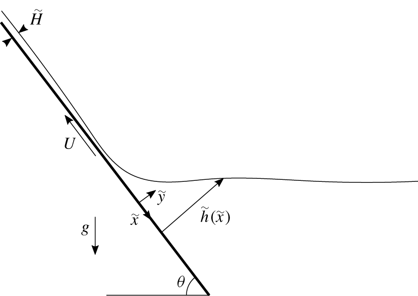
A schematic diagram of the plate withdrawal problem.

Consider an infinite flat plate inclined at angle  $0<\unicode[STIX]{x1D703}\leqslant \unicode[STIX]{x03C0}/2$ to the horizontal, partially submerged in a bath of fluid of viscosity
 $\unicode[STIX]{x1D707}$ and density
 $\unicode[STIX]{x1D70C}$, as shown in figure 1. A thin inextensible elastic sheet of bending stiffness
 $B$ lies over the surface of the fluid and up onto the exposed portion of the plate. The plate is withdrawn from the bath at constant speed
 $U$ in its own plane.
By analogy with the classical Landau–Levich problem, we expect the flow to develop towards a steady state in which a thin film of fluid is maintained between the plate and the sheet. We therefore look for steady solutions in which the fluid film tends to a constant, a priori unknown, depth  $\tilde{H}$ far upslope of the bath. The fluid is incompressible and obeys the steady Navier–Stokes equations,
 $$\begin{eqnarray}\displaystyle & \displaystyle \unicode[STIX]{x1D735}\boldsymbol{\cdot }\tilde{\boldsymbol{u}}=0, & \displaystyle\end{eqnarray}$$
 $$\begin{eqnarray}\displaystyle & \displaystyle \unicode[STIX]{x1D70C}\tilde{\boldsymbol{u}}\boldsymbol{\cdot }\unicode[STIX]{x1D735}\tilde{\boldsymbol{u}}=-\unicode[STIX]{x1D735}\tilde{p}+\unicode[STIX]{x1D707}\unicode[STIX]{x1D6FB}^{2}\tilde{\boldsymbol{u}}+\unicode[STIX]{x1D70C}\boldsymbol{g}, & \displaystyle\end{eqnarray}$$
where  $\tilde{\boldsymbol{u}}$ is the velocity of the fluid,
 $\tilde{p}$ is the pressure and
 $\boldsymbol{g}$ is the gravitational acceleration.
We take axes aligned with the plate, with  ${\tilde{y}}=0$ on the surface of the plate,
 $\tilde{x}\rightarrow \infty$ into the bath and
 $\tilde{x}\rightarrow -\infty$ into the film (see figure 1). The elastic sheet is located at a depth
 ${\tilde{y}}=\tilde{h}(\tilde{x})$ which satisfies the far-field conditions
 $$\begin{eqnarray}\displaystyle & \displaystyle \tilde{h}_{\tilde{x}}\rightarrow \tan \unicode[STIX]{x1D703}\quad \text{as }\tilde{x}\rightarrow \infty , & \displaystyle\end{eqnarray}$$
 $$\begin{eqnarray}\displaystyle & \displaystyle \tilde{h}\rightarrow \tilde{H}\quad \text{as }\tilde{x}\rightarrow -\infty , & \displaystyle\end{eqnarray}$$
where, throughout this work, subscripts denote partial derivatives.
The fluid cannot slip on, or penetrate, the plate or the sheet, so
 $$\begin{eqnarray}\displaystyle & \displaystyle \tilde{\boldsymbol{u}}=-U\hat{\boldsymbol{x}}\quad \text{at }{\tilde{y}}=0, & \displaystyle\end{eqnarray}$$
 $$\begin{eqnarray}\displaystyle & \displaystyle \tilde{\boldsymbol{u}}\boldsymbol{\cdot }\hat{\boldsymbol{t}}=-U,\quad \tilde{\boldsymbol{u}}\boldsymbol{\cdot }\hat{\boldsymbol{n}}=0\quad \text{at }{\tilde{y}}=\tilde{h}(\tilde{x}), & \displaystyle\end{eqnarray}$$
 $\hat{\boldsymbol{n}}=(-\tilde{h}_{\tilde{x}},1)/(1+\tilde{h}_{\tilde{x}}^{2})^{1/2}$ and
 $\hat{\boldsymbol{t}}=(1,\tilde{h}_{\tilde{x}})/(1+\tilde{h}_{\tilde{x}}^{2})^{1/2}$ are the unit normal and tangent vectors at the sheet respectively.
Here we have assumed there is no slippage between the sheet and the plate, so that far upslope the elastic sheet also moves at speed  $U$. One could apply other conditions at the sheet: other possible constraints are a stationary sheet, fixed over the bath, or a no-stress boundary condition to model an effective ‘sheet’ of surfactant molecules as in Dixit & Homsy (Reference Dixit and Homsy2013). These possible boundary conditions do not alter the general asymptotic structure of the solution. The minor changes that result from these different boundary conditions are given in § 3.2.
The dynamic condition at  ${\tilde{y}}=\tilde{h}$ is given by a balance in the normal stress across the inextensible sheet (see derivations by, e.g. Goldstein & Langer (Reference Goldstein and Langer1995) and Kaoui et al. (Reference Kaoui, Ristow, Cantat, Misbah and Zimmerman2008))
 $$\begin{eqnarray}\left.\hat{\boldsymbol{n}}\boldsymbol{\cdot }\tilde{\unicode[STIX]{x1D748}}\boldsymbol{\cdot }\hat{\boldsymbol{n}}\right|_{{\tilde{y}}=\tilde{h}(\tilde{x})}=-B\left(\frac{\unicode[STIX]{x2202}^{2}\tilde{\unicode[STIX]{x1D705}}}{\unicode[STIX]{x2202}\tilde{s}^{2}}+\frac{\tilde{\unicode[STIX]{x1D705}}^{3}}{2}\right),\end{eqnarray}$$
where  $\tilde{\unicode[STIX]{x1D748}}=-\tilde{p}\boldsymbol{I}+\unicode[STIX]{x1D707}[\unicode[STIX]{x1D735}\tilde{\boldsymbol{u}}+\unicode[STIX]{x1D735}\tilde{\boldsymbol{u}}^{\text{T}}]$ is the stress tensor,
 $\tilde{\unicode[STIX]{x1D705}}=\tilde{h}_{\tilde{x}\tilde{x}}/(1+\tilde{h}_{\tilde{x}}^{2})^{3/2}$ is the curvature, and
 $\tilde{s}$ is the parametrisation of the sheet shape by arclength, such that
 $$\begin{eqnarray}\frac{d}{\text{d}\tilde{s}}=\frac{1}{(1+\tilde{h}_{\tilde{x}}^{2})^{1/2}}\frac{d}{\text{d}\tilde{x}}.\end{eqnarray}$$
The  $\tilde{\unicode[STIX]{x1D705}}^{3}$ term arises from imposing inextensibility in the elastic sheet. A force balance along the sheet gives a material tension proportional to
 $\tilde{\unicode[STIX]{x1D705}}^{2}$, which acts on the curved interface to produce a force
 $\tilde{\unicode[STIX]{x1D705}}^{2}\tilde{\unicode[STIX]{x1D705}}$.
2.1 Non-dimensionalisation
We define an elasto-gravity length scale,  $l_{e}$, over which hydrostatic and elastic pressures balance in the absence of flow, and a visco-gravity length scale,
 $l_{v}$, over which viscous and gravitational forces balance in the presence of flow, as
 $$\begin{eqnarray}l_{e}=\left(\frac{B}{\unicode[STIX]{x1D70C}g}\right)^{1/4},\quad l_{v}=\left(\frac{\unicode[STIX]{x1D707}U}{\unicode[STIX]{x1D70C}g}\right)^{1/2}.\end{eqnarray}$$
The ratio of these length scales defines a non-dimensional number, similar to the capillary number in surface-tension driven flows, which we call the elasticity number
 $$\begin{eqnarray}El=\frac{l_{v}^{2}}{l_{e}^{2}}=\frac{\unicode[STIX]{x1D707}U}{(\unicode[STIX]{x1D70C}gB)^{1/2}},\end{eqnarray}$$
(cf. Dixit & Homsy Reference Dixit and Homsy2013). Note that the elastic capillary number of Seiwert et al. (Reference Seiwert, Quere and Clanet2013), who study a related situation with a finite sheet of length  $L$, is given similarly as
 $l_{v}^{2}L^{2}/l_{e}^{4}$, which reduces to
 $El$ if
 $L\sim l_{e}$.
In this paper we focus on the limit of a relatively stiff sheet or slow withdrawal speed,  $El\ll 1$, although we briefly discuss the effect of
 $El>O(1)$ in § 4. We further assume that the Reynolds number
 $Re=\unicode[STIX]{x1D70C}Ul_{e}/\unicode[STIX]{x1D707}$, defined with respect to the elasto-gravity length
 $l_{e}$, is not large (
 $ElRe\ll 1$), allowing us to neglect inertia throughout the following analysis.
2.2 Dimensionless equations
We scale lengths with the elasto-gravity length  $l_{e}$, velocities with the plate speed
 $U$ and pressure with the magnitude of the bending pressure,
 $B/l_{e}^{3}$, so that the governing equations, (2.1)–(2.2), may be written in terms of dimensionless (tilde-free) variables,
 $$\begin{eqnarray}\displaystyle & \displaystyle u_{x}+v_{y}=0, & \displaystyle\end{eqnarray}$$
 $$\begin{eqnarray}\displaystyle & \displaystyle -p_{x}+El\unicode[STIX]{x1D6FB}^{2}u+\sin \unicode[STIX]{x1D703}=O(ElRe), & \displaystyle\end{eqnarray}$$
 $$\begin{eqnarray}\displaystyle & \displaystyle -p_{y}+El\unicode[STIX]{x1D6FB}^{2}v-\cos \unicode[STIX]{x1D703}=O(ElRe), & \displaystyle\end{eqnarray}$$
with boundary conditions (2.3)–(2.6) now written as
 $$\begin{eqnarray}\displaystyle & \displaystyle h_{x}\rightarrow \tan \unicode[STIX]{x1D703}\quad \text{as }x\rightarrow \infty , & \displaystyle\end{eqnarray}$$
 $$\begin{eqnarray}\displaystyle & \displaystyle h\rightarrow H\quad \text{as }x\rightarrow -\infty , & \displaystyle\end{eqnarray}$$
 $$\begin{eqnarray}\displaystyle & \displaystyle u=-1,\quad v=0\quad \text{at }y=0, & \displaystyle\end{eqnarray}$$
 $$\begin{eqnarray}\displaystyle & \displaystyle \frac{u+h_{x}v}{(1+h_{x}^{2})^{1/2}}=-1,\quad v-h_{x}u=0\quad \text{at }y=h(x), & \displaystyle\end{eqnarray}$$
 $$\begin{eqnarray}p-\frac{2El}{(1+h_{x}^{2})}[u_{x}(h_{x}^{2}-1)-(u_{y}+v_{x})h_{x}]=\unicode[STIX]{x1D705}_{ss}+\frac{1}{2}\unicode[STIX]{x1D705}^{3}\quad \text{at }y=h(x),\end{eqnarray}$$
where  $\unicode[STIX]{x1D705}=h_{xx}/(1+h_{x}^{2})^{3/2}$ and
 $ds=\sqrt{1+h_{x}^{2}}\,dx$.
The solution  $h(x)$ therefore depends only on the two parameters
 $El$ and
 $\unicode[STIX]{x1D703}$. We determine the dimensionless film thickness
 $H$ as part of the solution
 $h(x)$.
3 Solution structure
The fluid bath is large and deep, so that far from the plate we expect the elastic lid to behave statically. Hydrostatic pressure balances the bending stresses here, and there is no flow. Near to the plate, however, fluid does flow in a film and we expect the force exerted by the elastic sheet to instead balance viscous dissipation in the fluid. We therefore look for a solution comprising an outer static region, an inner viscous film region and a transition region between the two.
3.1 Outer static region
Far from the plate, equations (2.10)–(2.16), to leading order in  $El$, provide a static balance between pressure gradients and gravity,
 $$\begin{eqnarray}\displaystyle & \displaystyle 0=-p_{x}+\sin \unicode[STIX]{x1D703}, & \displaystyle\end{eqnarray}$$
 $$\begin{eqnarray}\displaystyle & \displaystyle 0=-p_{y}-\cos \unicode[STIX]{x1D703}, & \displaystyle\end{eqnarray}$$
 $$\begin{eqnarray}\displaystyle & \displaystyle p=\unicode[STIX]{x1D705}_{ss}+{\textstyle \frac{1}{2}}\unicode[STIX]{x1D705}^{3}\quad \text{at }y=h. & \displaystyle\end{eqnarray}$$
Integrating (3.2) gives the pressure field
 $$\begin{eqnarray}p=\cos \unicode[STIX]{x1D703}(h-y)+\unicode[STIX]{x1D705}_{ss}+{\textstyle \frac{1}{2}}\unicode[STIX]{x1D705}^{3},\end{eqnarray}$$
and hence, from (3.1),
 $$\begin{eqnarray}\cos \unicode[STIX]{x1D703}h_{x}-\sin \unicode[STIX]{x1D703}+(1+h_{x}^{2})^{1/2}\left(\unicode[STIX]{x1D705}_{ss}+{\textstyle \frac{1}{2}}\unicode[STIX]{x1D705}^{3}\right)_{s}=0,\end{eqnarray}$$
which, given that  $\unicode[STIX]{x1D705}\sim h_{xx}$, is a fifth-order equation for
 $h$.
For a static elastic sheet meeting an inclined plate without adhesion, the relevant boundary conditions are zero depth, slope and curvature at the point of contact  $x=0$,
 $$\begin{eqnarray}\displaystyle h(0)=h_{x}(0)=h_{xx}(0)=0, & & \displaystyle\end{eqnarray}$$
and constant far-field slope
 $$\begin{eqnarray}h_{x}\rightarrow \tan \unicode[STIX]{x1D703}\quad \text{as }x\rightarrow \infty .\end{eqnarray}$$
The four conditions (3.6)–(3.7) in fact provide the five constraints needed. The linearisation of (3.5) in the far field is
 $$\begin{eqnarray}h_{xxxxx}+(1+\tan ^{2}\unicode[STIX]{x1D703})^{5/2}(\cos \unicode[STIX]{x1D703}h_{x}-\sin \unicode[STIX]{x1D703})=0,\end{eqnarray}$$
which has five exponential solutions, of which three decay as  $x\rightarrow \infty$. Eliminating the two growing modes as
 $x\rightarrow \infty$ therefore imposes two constraints.
We note that the choice of origin,  $x=0$, is arbitrary as the equations are translationally invariant. For convenience we choose it to be at the location of the point of contact as defined by (3.6). Other authors (e.g. Dixit & Homsy Reference Dixit and Homsy2013) make the equivalent choice of defining the origin elsewhere in the set-up, and solve for the distance to the point of contact.
We do not have the freedom to impose that any further derivatives vanish at the point of contact. This apparent imbalance is resolved by the existence of the inner region, onto which these higher-order derivatives match. In fact, we can solve analytically for the first non-zero derivative at  $x=0$, the shear stress in the sheet
 $S_{0}(\unicode[STIX]{x1D703})\equiv h_{xxx}(0)$. We multiply (3.5) by
 $\unicode[STIX]{x1D705}$
 $$\begin{eqnarray}(\cos \unicode[STIX]{x1D703}h_{x}-\sin \unicode[STIX]{x1D703})\frac{h_{xx}}{(1+h_{x}^{2})^{3/2}}+(1+h_{x}^{2})^{1/2}\unicode[STIX]{x1D705}\left(\unicode[STIX]{x1D705}_{ss}+\frac{1}{2}\unicode[STIX]{x1D705}^{3}\right)_{s}=0,\end{eqnarray}$$
and integrate with respect to  $s$ to find
 $$\begin{eqnarray}\displaystyle -\frac{(\sin \unicode[STIX]{x1D703}h_{x}+\cos \unicode[STIX]{x1D703})}{(1+h_{x}^{2})^{1/2}}+\unicode[STIX]{x1D705}\unicode[STIX]{x1D705}_{ss}-\frac{1}{2}\unicode[STIX]{x1D705}_{s}^{2}+\frac{3}{8}\unicode[STIX]{x1D705}^{4}=-1, & & \displaystyle\end{eqnarray}$$
where the constant follows from the boundary conditions in the far field,  $\unicode[STIX]{x1D705},\unicode[STIX]{x1D705}_{s}\rightarrow 0$ and
 $h_{x}\rightarrow \tan \unicode[STIX]{x1D703}$ as
 $x\rightarrow \infty$.
Since  $h_{x}=\unicode[STIX]{x1D705}=0$ at
 $x=0$, the gradient in curvature at the origin is
 $$\begin{eqnarray}\unicode[STIX]{x1D705}_{s}|_{x=0}=(2-2\cos \unicode[STIX]{x1D703})^{1/2},\end{eqnarray}$$
and so, given  $h_{x}(0)=h_{xx}(0)=0$, we deduce that
 $$\begin{eqnarray}S_{0}(\unicode[STIX]{x1D703})=(2-2\cos \unicode[STIX]{x1D703})^{1/2}.\end{eqnarray}$$
That is, the sheet approaches the plate with a non-zero shear stress  $h_{xxx}(0)$, which must then match with the viscous inner solution. This corrects the analysis of Dixit & Homsy (Reference Dixit and Homsy2013), who attempted to additionally impose zero shear stress on the outer solution at the point of contact, which the above calculation shows cannot hold.
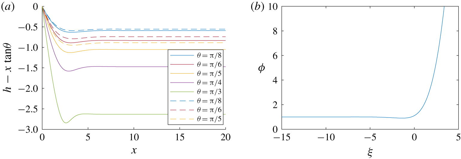
Further analytic progress beyond (3.10) is intractable, so we solve (3.5) numerically. Profiles of  $h(x)$ for a range of
 $\unicode[STIX]{x1D703}$ are shown in figure 2.
In the limit of small slope ( $\unicode[STIX]{x1D703}\ll 1$), the resulting deflections are small (
 $h_{x}\ll 1$) and the linearisation in (3.8) holds all the way to the plate, and reduces to
 $$\begin{eqnarray}h_{xxxxx}+(h_{x}-\unicode[STIX]{x1D703})+O(\unicode[STIX]{x1D703}^{3})=0,\end{eqnarray}$$
with exact solution
 $$\begin{eqnarray}h=\sqrt{2}\unicode[STIX]{x1D703}\left[\exp \left(-\frac{x}{\sqrt{2}}\right)\cos \left(\frac{x}{\sqrt{2}}\right)-1\right]+\unicode[STIX]{x1D703}x.\end{eqnarray}$$
This fits closely to the full profile of  $h$ for small
 $\unicode[STIX]{x1D703}$ (figure 2). The shear stress at
 $x=0$ is
 $S_{0}=\unicode[STIX]{x1D703}+O(\unicode[STIX]{x1D703}^{3}),$ in agreement with (3.12).


3.2 Inner region
Near the plate, viscous stresses are no longer negligible, and the dynamics are therefore fundamentally controlled by a balance between elastic stresses determined by the bending of the sheet as it approaches the plate and viscous stresses in the thin-film flow. Hence, in the inner region near the plate, we anticipate that viscous drag balances along-plate pressure gradients, and so, from (2.11),  $p/x\sim El(u/y^{2})$. Since the pressure is still dominated by the bending pressure,
 $p\sim h/x^{4}.$ The plate imposes unit speed
 $u\sim 1$, and the requirement of matching the shear stress of the outer region indicates that
 $h/x^{3}\sim 1$. Scaling
 $h\sim y$, we therefore define rescaled variables as
 $$\begin{eqnarray}\bar{u}=u,\quad \bar{v}=\frac{v}{El^{1/2}},\quad \bar{x}=\frac{x}{El^{1/4}},\quad (\bar{y},\bar{h},\bar{H})=\frac{(y,h,H)}{El^{3/4}},\quad \bar{p}=El^{1/4}p.\end{eqnarray}$$
The main difference between this and the capillary Landau–Levich problem is that scaling of the forcing (here the shear, there the curvature) does not match the pressure scale, so the pressure is rescaled. This requires the pressure in the inner region to vanish in order to match across scales. We note that this generic matching behaviour is not unusual for problems involving elasticity (e.g. Seiwert et al. Reference Seiwert, Quere and Clanet2013).
In contrast, if the scaling were chosen so that pressure remained unscaled, as in Dixit & Homsy (Reference Dixit and Homsy2013), it would be the shear stress of the outer solution, which we have already calculated to be non-zero, that would have to vanish to match across scales. This is clearly inconsistent.
In terms of the rescaled variables, (3.15), to leading order in  $El$, equations (2.10)–(2.16) become
 $$\begin{eqnarray}\displaystyle & \displaystyle \bar{u}_{\bar{x}}+\bar{v}_{\bar{y}}=0, & \displaystyle\end{eqnarray}$$
 $$\begin{eqnarray}\displaystyle & \displaystyle 0=-\bar{p}_{\bar{x}}+\bar{u}_{\bar{y}\bar{y}}, & \displaystyle\end{eqnarray}$$
 $$\begin{eqnarray}\displaystyle & \displaystyle 0=-\bar{p}_{\bar{y}}, & \displaystyle\end{eqnarray}$$
 $$\begin{eqnarray}\displaystyle \bar{u}=-1,\quad \bar{v}=0\quad \text{at }\bar{y}=0,\bar{h}(\bar{x}), & & \displaystyle\end{eqnarray}$$
 $$\begin{eqnarray}\displaystyle & \displaystyle \bar{p}=\bar{h}_{\bar{x}\bar{x}\bar{x}\bar{x}}\quad \text{at }\bar{y}=\bar{h}(\bar{x}), & \displaystyle\end{eqnarray}$$
with
 $$\begin{eqnarray}\bar{h}\rightarrow \bar{H}\quad \text{as }\bar{x}\rightarrow -\infty .\end{eqnarray}$$
We can integrate across the film to find first the pressure gradient and then the flux
 $$\begin{eqnarray}\bar{q}=-\frac{\bar{h}^{3}}{12}\bar{p}_{\bar{x}}-\bar{h}=-\frac{\bar{h}^{3}}{12}\bar{h}_{\bar{x}\bar{x}\bar{x}\bar{x}\bar{x}}-\bar{h}.\end{eqnarray}$$
In steady state, the flux is constant through the film, so matching to the far-field depth  $\bar{h}\rightarrow \bar{H}$ as
 $\bar{x}\rightarrow -\infty$ gives
 $$\begin{eqnarray}\bar{h}_{\bar{x}\bar{x}\bar{x}\bar{x}\bar{x}}=-\frac{12(\bar{h}-\bar{H})}{\bar{h}^{3}}.\end{eqnarray}$$
After rescaling by the unknown far-field depth and corresponding peeling length scale via
 $$\begin{eqnarray}\unicode[STIX]{x1D719}=\frac{\bar{h}}{\bar{H}},\quad \unicode[STIX]{x1D709}=\frac{12^{1/5}\bar{x}}{\bar{H}^{3/5}},\end{eqnarray}$$
we arrive at the unitary elastic Landau–Levich equation
 $$\begin{eqnarray}\unicode[STIX]{x1D719}_{\unicode[STIX]{x1D709}\unicode[STIX]{x1D709}\unicode[STIX]{x1D709}\unicode[STIX]{x1D709}\unicode[STIX]{x1D709}}=-\frac{(\unicode[STIX]{x1D719}-1)}{\unicode[STIX]{x1D719}^{3}}\end{eqnarray}$$
also derived in Seiwert et al. (Reference Seiwert, Quere and Clanet2013) and Lister et al. (Reference Lister, Peng and Neufeld2013).
By linearising about  $\unicode[STIX]{x1D719}\rightarrow 1$ as
 $\unicode[STIX]{x1D709}\rightarrow -\infty$, we can see that the requirement that
 $\unicode[STIX]{x1D719}$ decays to a constant depth provides three constraints to eliminate each growing mode. A fourth boundary condition is set by the free choice of origin, leaving just one boundary condition to impose as
 $\unicode[STIX]{x1D709}\rightarrow \infty$.
As  $\unicode[STIX]{x1D719}\rightarrow \infty$,
 $\unicode[STIX]{x1D719}_{\unicode[STIX]{x1D709}\unicode[STIX]{x1D709}\unicode[STIX]{x1D709}\unicode[STIX]{x1D709}\unicode[STIX]{x1D709}}\rightarrow 0$, so in general solutions tend to quartic polynomials in
 $\unicode[STIX]{x1D709}$,
 $$\begin{eqnarray}\unicode[STIX]{x1D719}\rightarrow A_{0}\unicode[STIX]{x1D709}^{4}+B_{0}\unicode[STIX]{x1D709}^{3}+O(\unicode[STIX]{x1D709}^{2})\quad \text{as }\unicode[STIX]{x1D709}\rightarrow \infty ,\end{eqnarray}$$
and the final boundary condition determines the value of  $A_{0}$. We wish to match shear stresses between regions, but the pressure, a higher derivative, is lower order in
 $El$. Thus, to match the pressure between regions and across scales, we must impose
 $A_{0}=0$. This prevents the leading-order pressure contribution,
 $p\sim A_{0}El^{-1/4}$, from diverging.
We obtain  $\unicode[STIX]{x1D719}(\unicode[STIX]{x1D709})$ by integrating (3.25) numerically, as shown in figure 2. The scaled shear stress in the far field is determined from this solution to be
 $$\begin{eqnarray}\unicode[STIX]{x1D719}_{\unicode[STIX]{x1D709}\unicode[STIX]{x1D709}\unicode[STIX]{x1D709}}\rightarrow 6B_{0}=0.8325.\end{eqnarray}$$
Given this far-field constraint, we can solve for  $\bar{H}$ by matching the shear stress between inner and outer solutions,
 $$\begin{eqnarray}\displaystyle \lim _{\bar{x}\rightarrow \infty }\bar{h}_{\bar{x}\bar{x}\bar{x}}=\lim _{x\rightarrow 0}h_{xxx} & & \displaystyle\end{eqnarray}$$
to deduce that
 $$\begin{eqnarray}\displaystyle \bar{H}=12^{3/4}\left(\frac{6B_{0}}{S_{0}(\unicode[STIX]{x1D703})}\right)^{5/4}, & & \displaystyle\end{eqnarray}$$
or
 $$\begin{eqnarray}\displaystyle H=12^{3/4}\frac{0.8325^{5/4}}{(2-2\cos \unicode[STIX]{x1D703})^{5/8}}El^{3/4}. & & \displaystyle\end{eqnarray}$$
We note that altering the boundary conditions at the sheet would change only the numerical prefactor of  $12^{3/4}$ in this expression: instead of (3.22), a stationary sheet would give
 $\bar{q}=-\frac{1}{12}\bar{h}_{\bar{x}\bar{x}\bar{x}\bar{x}\bar{x}}\bar{h}^{3}-\frac{1}{2}\bar{h}$, and a prefactor of
 $6^{3/4}$ in (3.29), while a no-stress boundary, as used by Dixit & Homsy (Reference Dixit and Homsy2013), leads to
 $\bar{q}=-\frac{1}{3}\bar{h}_{\bar{x}\bar{x}\bar{x}\bar{x}\bar{x}}\bar{h}^{3}-\bar{h}$ and a prefactor of
 $3^{3/4}$. The scaling
 $H\sim El^{3/4}$ agrees with the similar result of Seiwert et al. (Reference Seiwert, Quere and Clanet2013) and corrects the
 $H\sim El^{4/7}$ arrived at by Dixit & Homsy (Reference Dixit and Homsy2013).
3.3 Numerical simulations for  $\unicode[STIX]{x1D703}\ll 1$

As a verification of our predicted scaling for the film thickness with  $El$, we return to the case
 $\unicode[STIX]{x1D703}\ll 1$. Here there is a natural separation of scales between the horizontal and vertical, and we can use lubrication theory all the way from the inner viscous film out to the (shallow) bath.
To leading order in  $\unicode[STIX]{x1D703}\sim y/x$, (2.11)–(2.16) become
 $$\begin{eqnarray}\displaystyle & \displaystyle -p_{x}+Elu_{yy}+\sin \unicode[STIX]{x1D703}=0, & \displaystyle\end{eqnarray}$$
 $$\begin{eqnarray}\displaystyle & \displaystyle -p_{y}-\cos \unicode[STIX]{x1D703}=0, & \displaystyle\end{eqnarray}$$
 $$\begin{eqnarray}\displaystyle & \displaystyle u=-1\quad \text{at }y=0,h(x), & \displaystyle\end{eqnarray}$$
 $$\begin{eqnarray}\displaystyle & \displaystyle p=h_{xxxx}\quad \text{at }y=h(x). & \displaystyle\end{eqnarray}$$
As in (3.22) we integrate across the film to find the flux
 $$\begin{eqnarray}q=-\frac{h^{3}}{12El}\left(h_{xxxxx}+\cos \unicode[STIX]{x1D703}h_{x}-\sin \unicode[STIX]{x1D703}\right)-h=\frac{H^{3}}{12El}\sin \unicode[STIX]{x1D703}-H,\end{eqnarray}$$
which differs from (3.22) only in the inclusion of gravity. Here we give this equation in terms of the outer dimensionless variables to highlight that this continues to hold over the shallow bath.
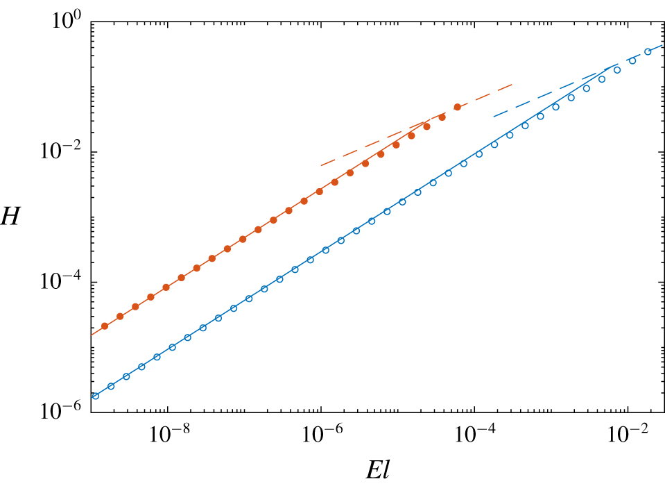
Numerical solutions of the  $\unicode[STIX]{x1D703}\ll 1$ problem (3.35) for
 $\unicode[STIX]{x1D703}=\unicode[STIX]{x03C0}/30$ (red filled circles) and
 $\unicode[STIX]{x1D703}=\unicode[STIX]{x03C0}/5$ (blue open circles), together with the predicted film thickness (3.30) (solid lines) for
 $El\ll 1$. The dashed lines show
 $H=H_{c}$ (4.4), above which there are no steady solutions, as discussed in § 4.

We integrate (3.35) numerically using MATLAB’s bvp4c routine, formulated as an eigenvalue problem for  $H$ and subject to boundary conditions (2.13)–(2.14) as
 $x\rightarrow \pm \infty$. In the limit
 $El\ll 1$, we obtain excellent agreement with the predicted scalings, including of the prefactor (see figure 3).
4 Breakdown of the asymptotics
In this paper we have calculated the steady-state film thickness in the limit  $El\ll 1$. When the film thickness becomes comparable to the visco-gravity length scale,
 $l_{e}\sim l_{v}$, or
 $El\sim 1$, we expect the asymptotics presented here to break down. It is no longer possible to neglect the effects of gravity in the inner region, as the dragged-out depth becomes large enough for gravity to play a role.
Further, we have assumed that a steady state is reached. If this experiment were performed in practice, there would be an initial contact point which is dragged upstream, below which a flow develops, and for  $El\ll 1$, reaches steady state. If
 $El$ is sufficiently large, we will instead see that the flow remains dependent on initial conditions everywhere.
To show how the inclusion of gravity causes a breakdown of the results presented thus far, we note that the flux in the inner region, including the effects of gravity, is
 $$\begin{eqnarray}q=-\frac{h^{3}}{12El}(h_{xxxxx}+\cos \unicode[STIX]{x1D703}h_{x}-\sin \unicode[STIX]{x1D703})-h=\frac{H^{3}}{12El}\sin \unicode[STIX]{x1D703}-H.\end{eqnarray}$$
Time dependence is introduced through an expression of mass conservation,
 $$\begin{eqnarray}\frac{\unicode[STIX]{x2202}h}{\unicode[STIX]{x2202}t}+\frac{\unicode[STIX]{x2202}q}{\unicode[STIX]{x2202}x}=0,\end{eqnarray}$$
which is a nonlinear advection–diffusion equation for  $h$, with a speed of information propagation given by
 $c=\text{d}q/\text{d}h$, which as
 $h\rightarrow H$ tends to
 $$\begin{eqnarray}c=\frac{1}{4El}\sin \unicode[STIX]{x1D703}H^{2}-1,\end{eqnarray}$$
from (4.1). Equation (4.3) suggests that information travels upslope for
 $$\begin{eqnarray}H<H_{c}(El,\unicode[STIX]{x1D703})\equiv \sqrt{4El/\sin \unicode[STIX]{x1D703}}.\end{eqnarray}$$
Since  $H\sim El^{3/4}/\unicode[STIX]{x1D703}^{5/4}$ (3.30), we can express this condition as
 $El\lesssim \unicode[STIX]{x1D703}^{3}$. Thus for sufficiently slow withdrawal speeds (small
 $El$), or on sufficiently steep slopes (large
 $\unicode[STIX]{x1D703}$), the initial conditions are swept upslope. Their influence is confined to a small nose region, eventually very far from the bath. This justifies solving for the steady state when
 $El\lesssim \unicode[STIX]{x1D703}^{3}$, and shows that the manner of exit of the plate from the bath controls upslope film thickness in this limit.
However, for faster plate speeds or lower slopes, such a scaling analysis suggests that in the resulting thicker film, information instead propagates down from the top of the film into the bath (the sign of (4.3) reverses). The flow produced by the withdrawal of the plate thus remains dependent on the initial conditions everywhere, even at late times. So a steady-state solution cannot develop, even in the limit of long drag-out times. It follows that on sufficiently shallow slopes, or at sufficiently fast plate speeds, dip coating under an elastic lid cannot produce a steady, uniform film. An analogous result holds for the classical capillary Landau–Levich problem, where steady solutions do not exist if the capillary number is too large (see the appendix of Jin, Acrivos & Münch Reference Jin, Acrivos and Münch2005).
In the time dependent problem, for  $El\ll \unicode[STIX]{x1D703}^{3}$, the steady film makes up the majority of dragged out region, and the contact point joins onto the film via a viscously dominated nose region. This nose has a self-similar parabolic shape found by solving (4.2) in the limit
 $h\ll 1$,
 $$\begin{eqnarray}\frac{\unicode[STIX]{x2202}h}{\unicode[STIX]{x2202}t}-\frac{\unicode[STIX]{x2202}h}{\unicode[STIX]{x2202}x}+\frac{\sin \unicode[STIX]{x1D703}}{El}\frac{\unicode[STIX]{x2202}h^{3}}{\unicode[STIX]{x2202}x}=0.\end{eqnarray}$$
The profile is given by
 $$\begin{eqnarray}h=\sqrt{\frac{4El(t-x)}{\sin \unicode[STIX]{x1D703}t}},\end{eqnarray}$$
and the length of the nose is found by matching its height onto the steady film depth found previously (see also de Ryck & Quere (Reference de Ryck and Quere1998)). Hence as  $El$ increases, the resulting increase in depth of the steady film gives a longer nose, until the nose engulfs the entire film and matches directly onto the bath at
 $x=0$, with a depth of
 $\sqrt{4El/\sin \unicode[STIX]{x1D703}}$. We thus recover the condition
 $H<H_{c}$ (4.4) for the existence of steady films. Moreover, we see that for
 $El\gtrsim \unicode[STIX]{x1D703}^{3}$, the solution instead takes the form of a parabolic nose matching onto the bath at
 $x=0$ and depth
 $H=H_{c}$.
There is another potential resolution to this loss of steady solutions at large  $El$. In this paper we have considered the case where the withdrawal of the plate determines the depth of the film. We could instead consider a situation in which the film depth upstream of the bath is imposed, and seek these alternative steady solutions (cf. Benilov et al. Reference Benilov, Chapman, McLeod, Ockendon and Zubkov2010). This would require information to be propagating from the film down the plate, and so from (4.3), the non-dimensional film depth would need to be at least
 $H>H_{c}$. In this case it is worth noting that the far-field depth would be set as a boundary condition, rather than being part of the solution. However, inspecting (4.1), the change of sign in wave speed occurs simultaneously with the appearance of an additional decaying root of the linearised system as
 $x\rightarrow -\infty$. Hence imposing the film depth is required for consistency, as anticipated, and so steady solutions exist in this case for any
 $H>H_{c}$.
5 Conclusions
In this paper, we have examined the elastic Landau–Levich problem, and found the leading-order solution for the film depth and surface profile as a function of the elasticity number  $El\ll 1$ and the plate angle
 $0<\unicode[STIX]{x1D703}<\unicode[STIX]{x03C0}/2$. The full, dimensional expression for the thickness of the film deposited on the withdrawn plate is
 $$\begin{eqnarray}\tilde{H}=\frac{\unicode[STIX]{x1D6FC}(\unicode[STIX]{x1D707}U)^{3/4}}{B^{1/8}[\unicode[STIX]{x1D70C}g(1-\cos \unicode[STIX]{x1D703})]^{5/8}},\end{eqnarray}$$
where the constant  $\unicode[STIX]{x1D6FC}$ depends on the choice of boundary condition on the elastic sheet (for the case of a sheet moving with the plate at speed
 $U$, as considered in this paper,
 $\unicode[STIX]{x1D6FC}=3.324$).
The key physical balances behind the scaling  $\tilde{H}\sim El^{3/4}l_{e}$ are of the shear stress between the inner film and the bath, and of viscous dissipation in the film to the bending-pressure gradients exerted by the sheet. While this elastic Landau–Levich problem shares many qualitative results with its classical capillary analogue, the process is governed by the balance in the shear stress rather than pressure between the inner film and the bath. This method of matching between regions applies more generally to processes involving elasticity and thin films of fluid.
Acknowledgements
The authors are very grateful to J. R. Lister and G. G. Peng for initially directing us towards this problem, and for many helpful discussions along the way. J.A.N. is partly supported by a Royal Society University Research Fellowship. K.L.P.W. is supported by the Natural Environment Research Council (grant no. NE/L002507/1).
Declaration of interests
The authors report no conflict of interest.