1 Introduction
A Riemann problem consists of an initial value problem composed of a set of conservation equations together with initial piecewise constant data having a single discontinuity.
In nonlinear shallow water flows, piecewise continuous solutions frequently develop. This is because the equations commonly used for describing them admit shocks (discontinuities) as solutions. These are usually interpreted as breaking waves (or bores), and therefore possess a straightforward physical significance, as well as a mathematical structure. These shocks are weak solutions in the sense that they satisfy the integral form of the flow equations. Smooth (differentiable) flow regions may be matched across these shocks by shock conditions, which can be derived by considering mass and momentum conservation across the shock.
Therefore, Riemann problems commonly occur in shallow water flows. Indeed, if one interprets all data in a shallow water numerical model as being piecewise continuous, then a whole series of such problems is solved at each time, and this interpretation forms the basis of a class of numerical shallow water solvers (Toro Reference Toro2001).
From a physical standpoint, Riemann solutions in shallow water flows are important because they provide us with solutions to idealised problems that can be used as verification cases for numerical solvers. Additionally, these idealised problems serve to highlight fundamental shallow water dynamics. In shallow water flows a variety of Riemann problems are of interest. Some of the simplest of these are dam-break problems, which comprise a Riemann problem with zero initial velocities.
The simplest dam-break problem involves one wet and one dry side (wet–dry), and with the point of discontinuity corresponding to the position of a notional dam wall that at the initial time is instantaneously removed. Solution to this simplest shallow water dam-break problem is given in Stoker (Reference Stoker1957). Although one could insist that a dam-break problem only be wet–dry, here we relax this description so as to include so-called wet–wet dam-break problems. These more generalised dam-break problems have a richer structure (see Toro Reference Toro2001). We further consider dam-break problems in which the initial bed levels also are different (see Bernetti, Titarev & Toro Reference Bernetti, Titarev and Toro2008).
The Riemann problems in Stoker (Reference Stoker1957), Toro (Reference Toro2001), Bernetti et al. (Reference Bernetti, Titarev and Toro2008) are those with a fixed bed. If we allow the bed to become erodible, coupling flow velocity to movement of sediment via a bed-load sediment transport relation, then a more complex picture emerges. The solution of the shallow water mobile-bed wet–dry dam-break problem with no bed discontinuity at the dam location dates back to Fraccarollo & Capart (Reference Fraccarollo and Capart2002), who considered a system with separate layers for fluid and sediment. The equivalent problem without separate layers was considered by Kelly & Dodd (Reference Kelly and Dodd2009), amongst others. These problems are also important from a physical perspective because in real dam-break events considerable scour may result due to the high flow velocities.
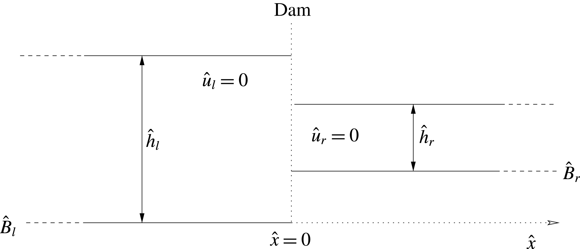
In this paper we go further and consider generalised mobile-bed dam-break problems, in which initial bed levels are not, in general, equal across the initial data: see figure 1. Aside from being important in the context of true dam-break events, they also have relevance in the dynamics of waves on a beach. This is because a so-called backwash bore (i.e. a hydraulic jump) is frequently created when water runs back down the beach after a single wave uprush (Hibberd & Peregrine Reference Hibberd and Peregrine1979). As the water drains the conditions at the hydraulic jump may be such that flow is minimal and thus subsequent development is predictable as a solution to a mobile-bed dam-break problem (Zhu & Dodd Reference Zhu and Dodd2015).
Schematic diagram for a dam-break problem.

Furthermore, we reconsider the usual shock conditions. For non-constant bed levels the bed-slope term in the flux-conservative form of the momentum equation is not integrable, necessitating approximation using conditions on each side of the shock. Here we reinterpret this term based on a new approximation of the internal shock structure. Although the motivation for this comes from the limiting case of flow over a sloping bed (and against which we subsequently verify the method), we instead approximate the internal morphodynamic shock structure as a series of sub-shock problems.
In the next section we present our governing equations, as well as some of the theory governing the determination of the wave structure across the evolving Riemann solution. We then use this theory to solve this class of Riemann problem in § 3. Finally we present conclusions.
2 Model development
2.1 Governing equations
A one-dimensional (1-D) idealised configuration for the initial set-up of a generalised dam-break problem is shown in figure 1. As mentioned, the nonlinear shallow water equations (NSWEs) have often been used for describing one- or two-dimensional dam-break flows (Ritter Reference Ritter1892; Stoker Reference Stoker1957; Toro Reference Toro2001; Bernetti et al. Reference Bernetti, Titarev and Toro2008). For dam-break problems over a mobile bed, and if only bed load is considered (see Soulsby Reference Soulsby1997), the governing equations are the NSWEs and a sediment-conservation equation:
 $$\begin{eqnarray}\displaystyle & \displaystyle {\hat{h}}_{\hat{t}}+\hat{u} {\hat{h}}_{\hat{x}}+{\hat{h}}\hat{u} _{\hat{x}}=0, & \displaystyle\end{eqnarray}$$
 $$\begin{eqnarray}\displaystyle & \displaystyle \hat{u} _{\hat{t}}+\hat{u} \hat{u} _{\hat{x}}+g{\hat{h}}_{\hat{x}}+g\hat{B}_{\hat{x}}=0, & \displaystyle\end{eqnarray}$$
 $$\begin{eqnarray}\displaystyle & \displaystyle \hat{B}_{\hat{t}}+\unicode[STIX]{x1D709}\hat{q}_{\hat{x}}=0, & \displaystyle\end{eqnarray}$$
where
 $\hat{x}$
represents horizontal distance (
 $\text{m}$
),
 $\hat{t}$
is time (
 $\text{s}$
),
 ${\hat{h}}$
represents water depth (
 $\text{m}$
),
 $\hat{u}$
is a depth-averaged horizontal velocity (
 $\text{m}~\text{s}^{-1}$
),
 $\hat{B}$
is the bed level (
 $\text{m}$
),
 $\hat{q}$
is sediment flux due to bed load (
 $\text{m}^{2}~\text{s}^{-1}$
),
 $\unicode[STIX]{x1D709}=1/(1-p)$
with
 $p$
being bed porosity and
 $g$
is acceleration due to gravity (
 $\text{m}~\text{s}^{-2}$
).
In order to reveal the shock dynamics by solving a strictly hyperbolic system, we do not include the downslope diffusion effect in our model, although morphodynamic shocks are considered where vertical bed steps occur.
In general,
 $\hat{q}$
is strongly dependent on
 $\hat{u}$
and a weak function of
 ${\hat{h}}$
. Here, a simple but commonly used formula
 $\hat{q}=A\hat{u} ^{3}$
(see Grass Reference Grass1981) is employed for the bed load (see e.g. Kelly & Dodd Reference Kelly and Dodd2010; Zhu, Dodd & Briganti Reference Zhu, Dodd and Briganti2012), with
 $A$
being the bed mobility parameter (
 $\text{s}^{2}~\text{m}^{-1}$
). Note that this formulation is an over-simplification of the complex process of bed-load transport (see e.g. Pritchard & Hogg Reference Pritchard and Hogg2005) but that the purpose here is to construct the mathematical solution so that the basic dynamics can be understood, and to provide a mathematical test case for numerical models.
Therefore, (2.3) becomes
 $$\begin{eqnarray}\displaystyle \hat{B}_{\hat{t}}+3\unicode[STIX]{x1D709}A\hat{u} ^{2}\hat{u} _{\hat{x}}=0. & & \displaystyle\end{eqnarray}$$
2.2 Non-dimensionalisation
The non-dimensional variables are
 $$\begin{eqnarray}\displaystyle x=\frac{\hat{x}}{{\hat{h}}_{0}},\quad t=\frac{\hat{t}}{{\hat{h}}_{0}^{1/2}g^{-1/2}},\quad h=\frac{{\hat{h}}}{{\hat{h}}_{0}},\quad u=\frac{\hat{u} }{\hat{u} _{0}}\quad \text{and}\quad B=\frac{\hat{B}}{{\hat{h}}_{0}}, & & \displaystyle\end{eqnarray}$$
where
 ${\hat{h}}_{0}$
is a length scale, and
 $\hat{u} _{0}=(g{\hat{h}}_{0})^{1/2}$
.
Substituting (2.5) into the governing equations (2.1), (2.2) and (2.4) gives
 $$\begin{eqnarray}\displaystyle & \displaystyle h_{t}+uh_{x}+hu_{x}=0, & \displaystyle\end{eqnarray}$$
 $$\begin{eqnarray}\displaystyle & \displaystyle u_{t}+uu_{x}+h_{x}+B_{x}=0, & \displaystyle\end{eqnarray}$$
 $$\begin{eqnarray}\displaystyle & \displaystyle B_{t}+3\unicode[STIX]{x1D70E}u^{2}u_{x}=0, & \displaystyle\end{eqnarray}$$
where
 $\unicode[STIX]{x1D70E}=\unicode[STIX]{x1D709}Ag$
.
The vector form of these three non-dimensional governing equations is
 $$\begin{eqnarray}\boldsymbol{U}_{t}+\boldsymbol{A}(\boldsymbol{U})\boldsymbol{U}_{x}=0,\end{eqnarray}$$
with
 $$\begin{eqnarray}\displaystyle \boldsymbol{U}=\left[\begin{array}{@{}c@{}}h\\ u\\ B\\ \end{array}\right],\quad \boldsymbol{A}(\boldsymbol{U})=\left[\begin{array}{@{}ccc@{}}u & h & 0\\ 1 & u & 1\\ 0 & 3\unicode[STIX]{x1D70E}u^{2} & 0\\ \end{array}\right]. & & \displaystyle\end{eqnarray}$$
The eigenvalues of
 $\boldsymbol{A}$
are the roots of the polynomial equation
 $$\begin{eqnarray}\unicode[STIX]{x1D706}^{3}-2u\unicode[STIX]{x1D706}^{2}+(u^{2}-3\unicode[STIX]{x1D70E}u^{2}-h)\unicode[STIX]{x1D706}+3\unicode[STIX]{x1D70E}u^{3}=0.\end{eqnarray}$$
Equation (2.11) has three roots, denoted
 $\unicode[STIX]{x1D706}_{1}$
,
 $\unicode[STIX]{x1D706}_{2}$
and
 $\unicode[STIX]{x1D706}_{3}$
such that
 $\unicode[STIX]{x1D706}_{1}\leqslant \unicode[STIX]{x1D706}_{3}\leqslant \unicode[STIX]{x1D706}_{2}$
. For the solution of
 $\unicode[STIX]{x1D706}_{1}$
,
 $\unicode[STIX]{x1D706}_{2}$
and
 $\unicode[STIX]{x1D706}_{3}$
we refer to Kelly & Dodd (Reference Kelly and Dodd2009, Reference Kelly and Dodd2010).
2.3 Generalised simple wave theory
When there are two equations or fewer in a Riemann problem, we can derive a Riemann invariant along each characteristic (Stoker Reference Stoker1957). Jeffrey (Reference Jeffrey1976) shows, however, that a direct extension of the concept of a Riemann invariant is not possible when there are more than two equations and dependent variables in a Riemann problem. Therefore, the generalised simple wave theory and the generalised Riemann invariants are introduced to solve such Riemann problems.
If we consider, for the moment, a general quasilinear hyperbolic system
 $$\begin{eqnarray}\boldsymbol{U}_{t}+\boldsymbol{A}(\boldsymbol{U})\boldsymbol{U}_{x}=0,\end{eqnarray}$$
where
 $\boldsymbol{U}$
is a vector of
 $n$
dependent variables, given by
 $$\begin{eqnarray}\boldsymbol{U}=[u_{1},u_{2},\ldots ,u_{n}]^{\text{T}},\end{eqnarray}$$
then the assumption that a simple wave region exists in a Riemann problem (or indeed generally) is such that
 $\boldsymbol{U}=\boldsymbol{U}(u_{1})$
holds across a wave, where
 $u_{1}$
is chosen without loss of generality. This means that there is a functional dependence between
 $u_{i}$
and
 $u_{1}$
of the form
 $u_{i}=f_{i}(u_{1})$
, and the wave is called a generalised simple wave (Jeffrey Reference Jeffrey1976). For a simple wave, equation (2.12) can be written as
 $$\begin{eqnarray}\left(\frac{\unicode[STIX]{x2202}u_{1}}{\unicode[STIX]{x2202}t}\boldsymbol{I}+\frac{\unicode[STIX]{x2202}u_{1}}{\unicode[STIX]{x2202}x}\boldsymbol{A}\right)\frac{\text{d}\boldsymbol{U}}{\text{d}u_{1}}=0.\end{eqnarray}$$
This system can have a non-trivial solution for
 $\text{d}\boldsymbol{U}/\text{d}u_{1}$
only if
 $$\begin{eqnarray}|\boldsymbol{A}-\unicode[STIX]{x1D706}_{i}\boldsymbol{I}|=0,\end{eqnarray}$$
where
 $$\begin{eqnarray}\unicode[STIX]{x1D706}_{i}=-\!\left(\frac{\unicode[STIX]{x2202}u_{1}}{\unicode[STIX]{x2202}t}\right)\left/\left(\frac{\unicode[STIX]{x2202}u_{1}}{\unicode[STIX]{x2202}x}\right),\quad i=1,2,\ldots ,n\Rightarrow \frac{\text{d}u_{1}}{\text{d}t}=0\text{ along }\frac{\text{d}x}{\text{d}t}=\unicode[STIX]{x1D706}_{i}.\right.\end{eqnarray}$$
This implies that
 $u_{1}$
, and therefore
 $u_{i}$
, are constant along characteristics
 $(\text{d}x/\text{d}t)=\unicode[STIX]{x1D706}_{i}$
, which are themselves straight lines. A simple wave can also be defined as the wave, across which one family of characteristics are all straight lines. There are
 $n$
families of characteristics, and the simple wave associated with the
 $i\text{th}$
characteristic family is called the
 $\unicode[STIX]{x1D706}_{i}$
simple wave.
From (2.14), when
 $\unicode[STIX]{x1D706}=\unicode[STIX]{x1D706}_{i}$
the vector
 $\text{d}\boldsymbol{U}/\text{d}u_{1}$
must be proportional to the right eigenvector
 $\boldsymbol{R}^{(i)}$
of
 $\boldsymbol{A}$
, which gives (Jeffrey Reference Jeffrey1976)
 $$\begin{eqnarray}\text{d}u_{j}=\frac{r_{j}^{(i)}}{r_{1}^{(i)}}\text{d}u_{1},\quad j=2,\ldots ,n,\end{eqnarray}$$
where
 $r_{j}^{(i)}$
is the
 $j$
th component of
 $\boldsymbol{R}^{(i)}$
.
Integrating (2.17) yields the
 $j$
th generalised Riemann invariant
 $K_{j}$
associated with the
 $\unicode[STIX]{x1D706}_{i}$
simple wave:
 $$\begin{eqnarray}u_{j}-\int \frac{r_{j}^{(i)}}{r_{1}^{(i)}}\,\text{d}u_{1}=K_{j},\quad j=2,\ldots ,n.\end{eqnarray}$$
Further details of the simple wave theory can be found in Jeffrey (Reference Jeffrey1976).
Returning to the present system we have
 $$\begin{eqnarray}\displaystyle \boldsymbol{R}^{(i)}=\left[\begin{array}{@{}c@{}}1\\ \displaystyle \frac{\unicode[STIX]{x1D706}_{i}-u}{h}\\ \displaystyle \frac{(\unicode[STIX]{x1D706}_{i}-u)^{2}}{h}-1\end{array}\right], & & \displaystyle\end{eqnarray}$$
and
 $$\begin{eqnarray}\displaystyle & \displaystyle \text{d}u=\frac{\unicode[STIX]{x1D706}_{i}-u}{h}\,\text{d}h & \displaystyle\end{eqnarray}$$
 $$\begin{eqnarray}\displaystyle & \displaystyle \text{d}B=\left(\frac{(\unicode[STIX]{x1D706}_{i}-u)^{2}}{h}-1\right)\,\text{d}h. & \displaystyle\end{eqnarray}$$
For a fixed
 $t$
, where
 $h$
varies continuously, equations (2.20) and (2.21) may be integrated across the
 $\unicode[STIX]{x1D706}_{i}$
simple wave, in the (
 $h$
,
 $u$
,
 $B$
) phase space, to yield the structure. However, variables do not always vary continuously across the Riemann structure. Therefore, we must understand the structure before we can solve it.
2.4 Wave structure for a Riemann problem
In general the Riemann problem associated with (2.12), is composed of
 $n$
waves associated with the
 $n$
characteristic families, which are separated by
 $n-1$
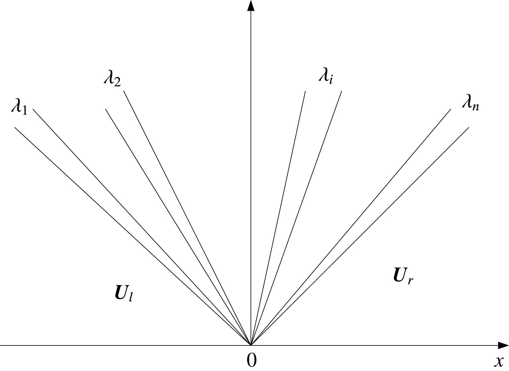
newly formed constant regions provided that the values in the initial piecewise constant states are sufficiently close (Lax Reference Lax1973; Fraccarollo & Capart Reference Fraccarollo and Capart2002; Toro Reference Toro2009): see figure 2. Note that a wave could be a rarefaction fan, a shock or a contact wave.
Wave structure for a Riemann problem with
 $n$
characteristic families.

As we integrate (2.20) and (2.21) across a
 $\unicode[STIX]{x1D706}_{i}$
simple wave,
 $\unicode[STIX]{x1D706}_{i}$
varies such that
 $\text{d}\unicode[STIX]{x1D706}_{i}=\sum (\unicode[STIX]{x2202}\unicode[STIX]{x1D706}_{i}/\unicode[STIX]{x2202}u_{j})\,\text{d}u_{j}$
, and in view of (2.17):
 $$\begin{eqnarray}\frac{\text{d}\unicode[STIX]{x1D706}_{i}}{\text{d}u_{1}}=\unicode[STIX]{x1D735}_{\boldsymbol{U}}\unicode[STIX]{x1D706}_{i}\boldsymbol{\cdot }\boldsymbol{R}^{(i)},\end{eqnarray}$$
where we have assumed, without loss of generality, that
 $r_{1}^{(i)}=1$
. Equation (2.22) therefore represents the rate of change of characteristic velocity across the
 $\unicode[STIX]{x1D706}_{i}$
wave. If
 $$\begin{eqnarray}\unicode[STIX]{x1D735}_{\boldsymbol{U}}\unicode[STIX]{x1D706}_{i}\boldsymbol{\cdot }\boldsymbol{R}^{(i)}\neq 0\quad \text{for all}~\boldsymbol{U},\end{eqnarray}$$
then the characteristic velocity increases or decreases continuously across the
 $\unicode[STIX]{x1D706}_{i}$
wave, thus implying the existence of either an expansion (rarefaction) wave, or a compressive wave (which becomes a shock ultimately). Then the
 $\unicode[STIX]{x1D706}_{i}$
wave field is said to be genuinely nonlinear (or convex) (Sharma Reference Sharma2010). Note that if
 $$\begin{eqnarray}\unicode[STIX]{x1D735}_{\boldsymbol{U}}\unicode[STIX]{x1D706}_{i}\boldsymbol{\cdot }\boldsymbol{R}^{(i)}=0,\quad \text{for all}~\boldsymbol{U},\end{eqnarray}$$
the wave field is said to be genuinely linear.
If we return again to the present system we find that
 $$\begin{eqnarray}\unicode[STIX]{x1D735}_{\boldsymbol{U}}\unicode[STIX]{x1D706}_{i}\boldsymbol{\cdot }\boldsymbol{R}^{(i)}=\left.\left\{\unicode[STIX]{x1D706}_{i}+\left\{2\unicode[STIX]{x1D706}_{i}^{2}-(2u-6\unicode[STIX]{x1D70E}u)\unicode[STIX]{x1D706}_{i}-9\unicode[STIX]{x1D70E}u^{2}\right\}\frac{(u-\unicode[STIX]{x1D706}_{i})}{h}\right\}\right/G,\end{eqnarray}$$
where
 $G=3\unicode[STIX]{x1D706}^{2}-4u\unicode[STIX]{x1D706}+(u^{2}-3\unicode[STIX]{x1D70E}u^{2}-h)$
, and it is therefore not clear that (2.25) will be strictly
 ${>}$
or
 ${<}0$
. In this case the problem is said to be non-convex (Sharma Reference Sharma2010). Note that this is in contrast to the classical (fixed-bed) shallow water system, wherein
 $$\begin{eqnarray}\unicode[STIX]{x1D735}_{\boldsymbol{U}}\unicode[STIX]{x1D706}_{-,+}\boldsymbol{\cdot }\boldsymbol{R}^{(-,+)}=\mp \frac{3}{2}\sqrt{\frac{1}{h}}.\end{eqnarray}$$
This implies that the solution to the dam-break problem resulting from the system (2.6)–(2.8) may possess semi-characteristic shocks (Sharma Reference Sharma2010).
2.5 Semi-characteristic shock
In general,
 $\unicode[STIX]{x1D735}_{\boldsymbol{U}}\unicode[STIX]{x1D706}_{i}\boldsymbol{\cdot }\boldsymbol{R}^{(i)}=f(u_{1})$
across a simple wave. If, as seems possible for (2.25),
 $f(u_{1})$
passes through 0, this implies that at a rarefaction fan, across which characteristics must diverge, a point is reached at which this can no longer happen because
 $(\text{d}\unicode[STIX]{x1D706}_{i}/\text{d}u_{1})=f(u_{1})=0$
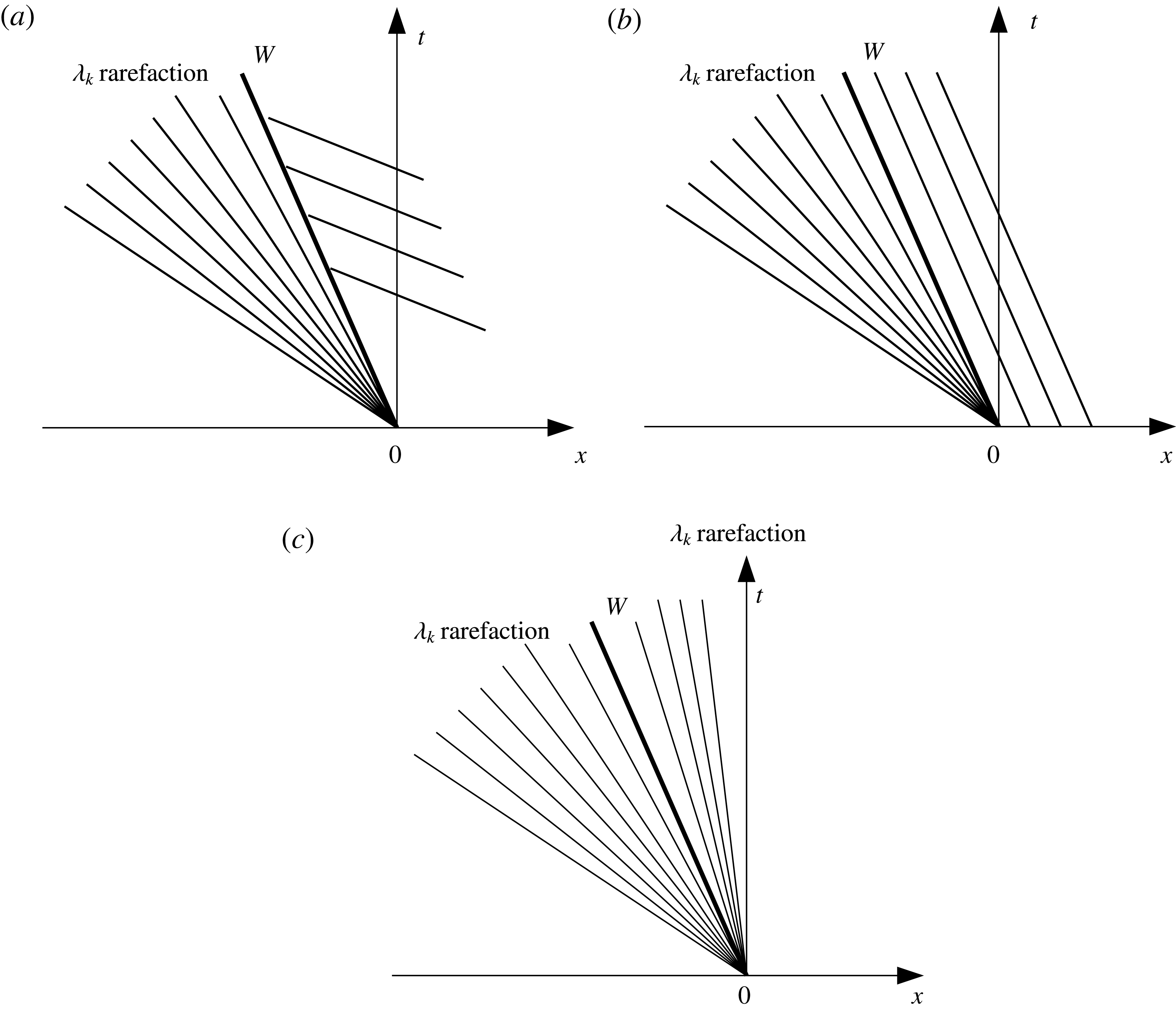
. The only way then of accommodating this behaviour without the solution becoming multivalued is for a shock to be contiguous with the fan: the semi-characteristic shock, with the characteristic at one edge of the fan coinciding with this semi-characteristic shock. The possible three wave structures are shown in figure 3. Note that only (a) represents a physical structure in general. This is because for figure 3(b,c) the structures will, in general, be overdetermined. For further details and exceptions see Sharma (Reference Sharma2010).
Schematic diagrams depicting possible structures for the combination of a rarefaction wave and a semi-characteristic shock within a simple wave.

2.6 Shock conditions
We require shock conditions to be satisfied across shocks and semi-characteristic shocks. For derivations of the shock conditions we refer to Kelly & Dodd (Reference Kelly and Dodd2010), Zhu et al. (Reference Zhu, Dodd and Briganti2012); the shock conditions are
 $$\begin{eqnarray}\displaystyle & \displaystyle h_{R}u_{R}-h_{L}u_{L}-(h_{R}-h_{L})W=0, & \displaystyle\end{eqnarray}$$
 $$\begin{eqnarray}\displaystyle & \displaystyle W(h_{R}u_{R}-h_{L}u_{L})-\left(h_{R}u_{R}^{2}+\frac{h_{R}^{2}}{2}-h_{L}u_{L}^{2}-\frac{h_{L}^{2}}{2}\right)-\int _{x_{L}}^{x_{R}}hB_{x}\,\text{d}x=0, & \displaystyle\end{eqnarray}$$
 $$\begin{eqnarray}\displaystyle & \displaystyle (B_{R}-B_{L})W-\unicode[STIX]{x1D70E}(u_{R}^{3}-u_{L}^{3})=0, & \displaystyle\end{eqnarray}$$
where
 $L$
and
 $R$
represent variables on the left and right side of a shock, and
 $W$
is shock velocity.
The term
 $\int _{x_{L}}^{x_{R}}hB_{x}\,\text{d}x=\int _{B_{L}}^{B_{R}}h\,\text{d}B$
is not uniquely determined, because
 $h(x,t)$
is not well defined along the face of bed step (Kelly Reference Kelly2009). Needham & Hey (Reference Needham and Hey1991) performed the integration by approximation:
 $$\begin{eqnarray}\int _{B_{L}}^{B_{R}}h\,\text{d}B\approx \frac{1}{2}(B_{R}-B_{L})(h_{R}+h_{L}).\end{eqnarray}$$
This expression is adopted by Kelly & Dodd (Reference Kelly and Dodd2010), Zhu et al. (Reference Zhu, Dodd and Briganti2012), Zhu & Dodd (Reference Zhu and Dodd2013, Reference Zhu and Dodd2015).
Bernetti et al. (Reference Bernetti, Titarev and Toro2008) equated it to the hydrostatic pressure force exerted on the bed step by the water:
 $$\begin{eqnarray}\displaystyle \int _{B_{L}}^{B_{R}}h\,\text{d}B=\left\{\begin{array}{@{}ll@{}}\displaystyle \frac{1}{2}h_{L}^{2}\quad & \text{if }B_{L}+h_{L}\leqslant B_{R},\\ \displaystyle \frac{1}{2}(B_{R}-B_{L})(2h_{L}+B_{L}-B_{R})\quad & \text{if }B_{R}\geqslant B_{L}\text{ and }B_{L}+h_{L}>B_{R},\\ \displaystyle \frac{1}{2}(B_{R}-B_{L})(2h_{R}+B_{R}-B_{L})\quad & \text{if }B_{R}<B_{L}\text{ and }B_{R}+h_{R}>B_{L},\\ \displaystyle \frac{1}{2}h_{R}^{2}\quad & \text{if }B_{R}+h_{R}\leqslant B_{L}.\end{array}\right. & & \displaystyle\end{eqnarray}$$
There are four cases depending on from which side the water is exerting a force on the bed step, and whether the free surface on the side of lower bed level is above the top of the bed step. Note that when free surface elevations on both sides are equal, equations (2.30) and (2.31) are identical.
Different interpretations are possible. This can be seen by assuming that in the vicinity of a sudden change in bed level (a bed step)
 $B=B_{L}+(B_{R}-B_{L})H(x-x_{0})$
, where
 $H(x)$
is the Heaviside function, so that
 $$\begin{eqnarray}B_{x}=(B_{R}-B_{L})\unicode[STIX]{x1D6FF}(x-x_{0}),\end{eqnarray}$$
where
 $\unicode[STIX]{x1D6FF}(x-x_{0})$
is the Dirac delta function, and
 $x=x_{0}$
is the location of the bed step. Using (2.32)
 $$\begin{eqnarray}\int _{x_{L}}^{x_{R}}hB_{x}\,\text{d}x=(B_{R}-B_{L})h(x_{0}).\end{eqnarray}$$
Therefore, the remaining ambiguity is in how to define
 $h(x_{0})$
. From this perspective the expression of Needham & Hey (Reference Needham and Hey1991) (hereinafter NH91) is a simple average depth across the discontinuity; similarly, the middle two of the expressions of Bernetti et al. (Reference Bernetti, Titarev and Toro2008) also correspond to composite depths, although the first and last cannot obviously be interpreted in this way. More generally, there is an implied variation of depth across the shock, which, it turns out, is important for the shocks we consider here.
2.7 Investigation of
 $\int _{x_{L}}^{x_{R}}hB_{x}\,\text{d}x$

If we know the internal structure of a shock, i.e.
 $h=h(B)$
across the shock, we can calculate the ambiguous integral numerically or analytically straightforwardly:
 $$\begin{eqnarray}\displaystyle \int _{B_{L}}^{B_{R}}h\,\text{d}B\approx \mathop{\sum }_{i=0}^{n-1}\bar{h}_{i}\unicode[STIX]{x0394}B_{i}=\mathop{\sum }_{i=0}^{n-1}\frac{1}{2}(h_{i}+h_{i+1})(B_{i+1}-B_{i}), & & \displaystyle\end{eqnarray}$$
where
 $h_{i}=h(B_{i})$
,
 $B_{0}\equiv B_{L}$
,
 $B_{n}\equiv B_{R}$
and here we take
 $\unicode[STIX]{x0394}B_{i}=(B_{R}-B_{L}/n)$
. When
 $n=1$
, it is the Needham & Hey (Reference Needham and Hey1991) approximation, i.e. (2.30). We refer to this approach as the
 $n$
-step approach; it is based on an implied internal structure of a shock. To see how this internal structure might be arrived at from a physical standpoint we now consider flow over a fixed-bed slope.
2.7.1 Interpretation of a stationary shock across a fixed-bed discontinuity
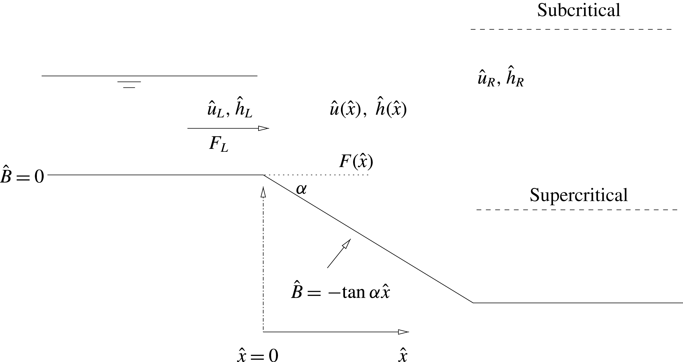
We consider a steady state flow across a fixed, linear slope (see figure 4), and therefore only the hydrodynamic behaviour. From shallow water theory, the flow over the slope is either entirely sub- or supercritical (see appendix D). We return here to dimensional variables, and then use an alternative non-dimensionalisation.
Bed level geometry for this case.
 $F=\hat{u} /\sqrt{g{\hat{h}}}$
is the Froude number. In these scenarios the whole flow is either sub- or supercritical.

From continuity we have
 $$\begin{eqnarray}{\hat{h}}(x)\hat{u} (x)={\hat{h}}_{L}\hat{u} _{L}=\hat{q}_{0}.\end{eqnarray}$$
For a steady state, the flux-conservative form of (2.2) is
 $$\begin{eqnarray}\{{\hat{h}}\hat{u} ^{2}+{\textstyle \frac{1}{2}}g{\hat{h}}^{2}\}_{\hat{x}}=-g{\hat{h}}\hat{B}_{\hat{x}}.\end{eqnarray}$$
Now we introduce a different set of non-dimensional variables
 $\tilde{h}$
,
 $\tilde{u}$
,
 $\tilde{x}$
and
 $\tilde{B}$
on the sloping section with
 ${\hat{h}}={\hat{h}}_{L}\tilde{h}$
,
 $\hat{u} =\hat{u} _{L}\tilde{u}$
,
 $\hat{x}={\hat{h}}_{L}\tilde{x}/\tan \unicode[STIX]{x1D6FC}$
and
 $\hat{B}={\hat{h}}_{L}\tilde{B}$
. This gives
 $$\begin{eqnarray}\tilde{u} =\frac{1}{\tilde{h}},\end{eqnarray}$$
 $$\begin{eqnarray}\tilde{B}=-\tilde{x},\end{eqnarray}$$
and
 $$\begin{eqnarray}\left\{F_{L}^{2}\frac{1}{\tilde{h}}+\frac{1}{2}\tilde{h}^{2}\right\}_{\tilde{x}}=-\tilde{h}\tilde{B}_{\tilde{x}}=\tilde{h}.\end{eqnarray}$$
Note that the slope
 $\tan \unicode[STIX]{x1D6FC}$
is now absent, and the only free parameter is the inflow Froude number,
 $F_{L}$
.
Straightforwardly, we then obtain
 $$\begin{eqnarray}\tilde{h}=1+\tilde{x}+\frac{1}{2}F_{L}^{2}\frac{(\tilde{h}^{2}-1)}{\tilde{h}^{2}}=1-\tilde{B}+\frac{1}{2}F_{L}^{2}\frac{(\tilde{h}^{2}-1)}{\tilde{h}^{2}}\end{eqnarray}$$
for the variation of
 $\tilde{h}$
across the slope. If we consider an abrupt change in bed level to be the limiting case as
 $\unicode[STIX]{x1D6FC}\rightarrow \unicode[STIX]{x03C0}/2$
of this linear slope variation, and, moreover, that this variation is independent of slope (
 $\tan \unicode[STIX]{x1D6FC}$
), we may then assume that this variation may be used across a fixed-bed step as the implied internal shock structure.
It should be noted that (2.40) can also be directly derived from an energy-conservation law for the shallow water equations, because the flow down the slope is continuous. There is some debate about whether energy conservation or the momentum balance equation, in which
 $\int _{\tilde{B}_{L}}^{\tilde{B}_{R}}\tilde{h}\,\text{d}\tilde{B}$
has to be approximated, should be used for the shock across a fixed-bed step (Cozzolino et al.
Reference Cozzolino, Morte, Covelli, Giudice and Pianese2011; Valiani & Caleffi Reference Valiani and Caleffi2017). The energy-conserving approach has been widely used to study the stationary shock across a fixed-bed discontinuity (Karelskii & Petrosyan Reference Karelskii and Petrosyan2006; Valiani & Caleffi Reference Valiani and Caleffi2017). Valiani & Caleffi (Reference Valiani and Caleffi2017) uses both energy conservation and momentum balance to derive a depth at the bed step, i.e.
 $h(x_{0})$
in (2.33). However, the energy loss across a morphodynamic shock is a priori unknown. Therefore in this work, we utilise the momentum equation to solve the stationary shock across a fixed-bed step and also for morphodynamic shocks. Accordingly, we now focus on the approximations for
 $\int _{\tilde{B}_{L}}^{\tilde{B}_{R}}\tilde{h}\,\text{d}\tilde{B}$
.
Equation (2.39) gives the exact solution of
 $$\begin{eqnarray}\int _{\tilde{B}_{L}}^{\tilde{B}_{R}}\tilde{h}\,\text{d}\tilde{B}=-\left[F_{L}^{2}\frac{1}{\tilde{h}}+\frac{1}{2}\tilde{h}^{2}\right]_{L}^{R},\end{eqnarray}$$
for a stationary shock across a fixed-bed discontinuity, in which
 $\tilde{h}$
is calculated using (2.40).
The exact solution (2.41) together with (2.40) allows us to see how well (2.30), (2.31) or (2.34) describe this usually ambiguous integral. The performances of these approximations are presented in appendix A, from which we can see that (2.34) yields greater accuracy than (2.30) or (2.31).
2.7.2 Application of
$n$
-step approach to morphodynamic shocks

In this section we consider whether the
 $n$
-step approach is valid for morphodynamic shocks. Hereafter we return to the non-dimensionalisation introduced in § 2.2.
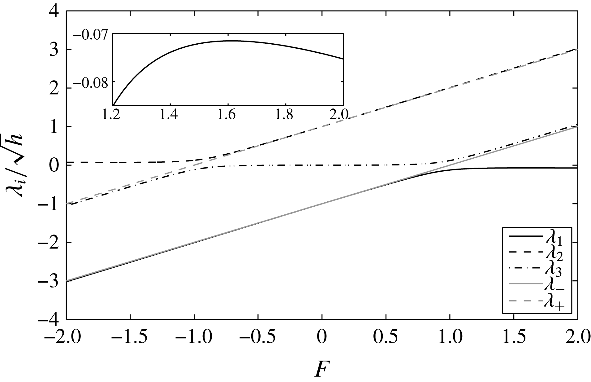
In the shallow water morphodynamical system that we consider here, there is in general one characteristic speed much smaller than the other two. This can be seen in figure 5, in which we plot
 $\unicode[STIX]{x1D706}^{\prime }=\unicode[STIX]{x1D706}/\sqrt{h}$
versus Froude number
 $F=u/\sqrt{h}$
. Note that the characteristic polynomial for
 $\unicode[STIX]{x1D706}^{\prime }$
depends only on
 $F$
and
 $\unicode[STIX]{x1D70E}$
:
 $$\begin{eqnarray}{\unicode[STIX]{x1D706}^{\prime }}^{3}-2F{\unicode[STIX]{x1D706}^{\prime }}^{2}+((1-3\unicode[STIX]{x1D70E})F^{2}-1)\unicode[STIX]{x1D706}^{\prime }+3\unicode[STIX]{x1D70E}F^{3}=0.\end{eqnarray}$$
The characteristic speed that is generally much smaller than the other two is associated with bed wave movement. This property pertains everywhere except for transcritical flows, as also indicated in figure 5. Here we define a morphodynamic shock as a shock formed by the convergence of two characteristics of one family, at least one of which is a bed characteristic, and for which the shock speed
 $|W|\ll 1$
.
Dimensionless characteristic velocities for our system with
 $\unicode[STIX]{x1D70E}=0.01$
(after Zhu & Dodd Reference Zhu and Dodd2015, figure 2).
 $\unicode[STIX]{x1D706}_{+,-}$
are the equivalent hydrodynamic (fixed-bed) characteristic velocities.

Now, note that
 $\unicode[STIX]{x1D70E}=\unicode[STIX]{x1D709}Ag\ll 1$
(see (2.8) and (2.29)). This is because
 $\hat{q}=O(10^{-3})~\text{m}^{3}~\text{s}^{-1}~\text{m}^{-1}$
or less, whereas
 $\hat{u} _{0}=O(1)~\text{m}~\text{s}^{-1}$
in our original non-dimensionalisation (2.5). This implies that at the hydrodynamical time scale
 $\hat{t}_{0}=\sqrt{{\hat{h}}_{0}/g}$
, equation (2.8) becomes
 $B_{t}\approx 0$
, implying no bed change at this time scale. However, at the morphodynamical time scale,
 $\hat{t}_{m}=\hat{t}_{0}/\unicode[STIX]{x1D70E}$
,
 $\Rightarrow$
both sides of (2.29) are of comparable magnitude. This is consistent with
 $W\ll 1$
for a morphodynamic shock, so that in these circumstances (2.27)–(2.29) become
 $$\begin{eqnarray}\displaystyle & \displaystyle h_{R}u_{R}-h_{L}u_{L}\approx 0, & \displaystyle\end{eqnarray}$$
 $$\begin{eqnarray}\displaystyle & \displaystyle -\!\left(h_{R}u_{R}^{2}+\frac{h_{R}^{2}}{2}-h_{L}u_{L}^{2}-\frac{h_{L}^{2}}{2}\right)-\int _{x_{L}}^{x_{R}}hB_{x}\,\text{d}x\approx 0, & \displaystyle\end{eqnarray}$$
 $$\begin{eqnarray}\displaystyle & \displaystyle (B_{R}-B_{L})W-\unicode[STIX]{x1D70E}(u_{R}^{3}-u_{L}^{3})=0. & \displaystyle\end{eqnarray}$$
Note that (2.43) and (2.44) are the same shock conditions as those for flow over a fixed-bed step. This implies (2.40) can be derived from (2.43) and (2.44). This scaling is equivalent to use of the quasi-steady approximation that is often used to study morphodynamics (see e.g. Ribas et al. Reference Ribas, Falqués, de Swart, Dodd, Garnier and Calvete2015). Therefore, we conclude that both (2.41) together with (2.40), and (2.34) with (2.40) in § 2.7.1, which are both for a fixed-bed stationary shock, can in principle be used as approximations for morphodynamic shocks with simplified shock conditions (2.43), (2.44) and (2.29). Note that the conversion between different non-dimensionalisations in § 2.7.1 and § 2.2 should be done before applying (2.41) and (2.40) for morphodynamic shocks.
By analogy, we can instead retain the
 $W$
terms in (2.27) and (2.28) to obtain the internal shock structures (
 $h_{i}$
,
 $u_{i}$
and
 $B_{i}$
) and apply the
 $n$
-step approach (2.34) for (2.27)–(2.29). In the remainder of this paper we use this approach, which we refer to as the
 $n$
-step approach, to construct the Riemann solution. The performances of these other approximations for morphodynamic shocks are examined in appendix C.
2.7.3 Implementation of
$n$
-step approach for morphodynamic shocks

To use (2.34) across a morphodynamic shock with (2.27)–(2.29), the procedure is as follows:
-
(i) Obtain initial estimates for
$\boldsymbol{U}_{R}=\boldsymbol{U}_{R}^{(1)}$
by solving (2.27)–(2.29), with
$\int _{x_{L}}^{x_{R}}hB_{x}\,\text{d}x$
approximated using (2.30). -
(ii)
$B_{i}$
values are then chosen according to
$B_{L}$
and
$B_{R}$
. Then
$h(B_{i})$
and
$u(B_{i})$
are calculated according to (2.27) and (2.28) for the known
$B_{i}$
, by replacing
$(h,u,B)_{iL}$
and
$(h,u,B)_{iR}$
by
$(h,u,B)_{i-1}$
and
$(h,u,B)_{i}$
. Note that
$(h,u,B)_{0}=(h,u,B)_{L}$
. -
(iii) Calculate the
$\int _{x_{L}}^{x_{R}}hB_{x}\,\text{d}x$
using the
$n$
-step approach (2.34). -
(iv) We then solve (2.27)–(2.29) using the calculated
$\int _{x_{L}}^{x_{R}}hB_{x}\,\text{d}x$
to get
$\boldsymbol{U}_{R}=\boldsymbol{U}_{R}^{(2)}$
. -
(v) Repeat (ii)–(iv) until
$\boldsymbol{U}_{R}$
converges.





3 Solution of dam-break problems over an initially piecewise flat mobile bed
The dam-break problem system consists of three equations, and according to Lax’s theorem (Lax Reference Lax1973) there are at most four constant states separated by three elementary waves associated with the three characteristic families. Note that for wet–dry dam-break problems over a mobile bed there are two waves separated by one newly formed constant region (Kelly & Dodd Reference Kelly and Dodd2009). One wave vanishes because of the presence of the dry bed.
3.1 Initial conditions
The dimensional initial conditions for a generalised dam-break problem are shown in figure 1. With
 ${\hat{h}}_{0}={\hat{h}}_{l}$
, the non-dimensional initial conditions of the left side are
 $h(x\leqslant 0)=h_{l}=1$
,
 $u(x\leqslant 0)=u_{l}=0$
,
 $B(x\leqslant 0)=B_{l}=0$
. For wet–dry dam-break problems,
 $h(x\geqslant 0)=h_{r}=0$
, and
 $u(x\geqslant 0)=u_{r}=0$
. For wet–wet dam-break problems, we set
 $h(x\geqslant 0)=h_{r}=0.1$
, and
 $u(x\geqslant 0)=u_{r}=0$
. In this paper, we consider conditions of both
 $B_{r}=0$
and
 $B_{r}\neq 0$
to investigate the wave structures in these more generalised dam-break problems.
3.2 Wet–dry dam-break problem
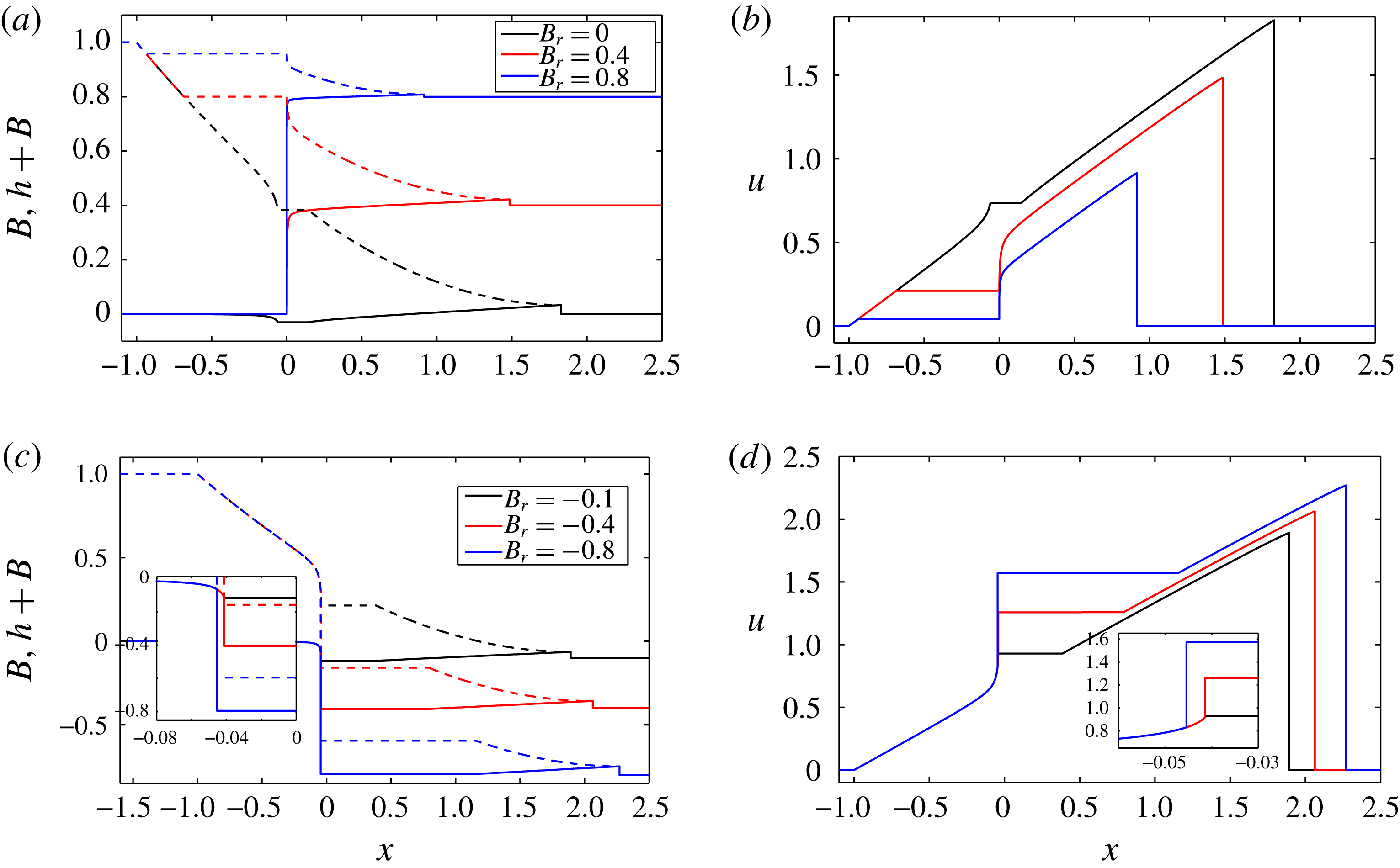
We first assume that the wet–dry dam-break solution over an erodible bed for various
 $B_{r}$
consists only of elementary waves, i.e. rarefaction waves or shocks. We introduce the semi-characteristic shock when the assumption no longer applies. The obtained wave structures at
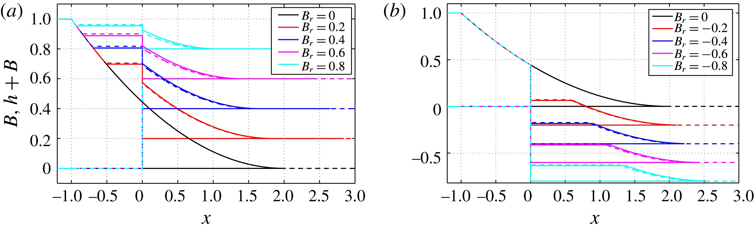
 $t=1$
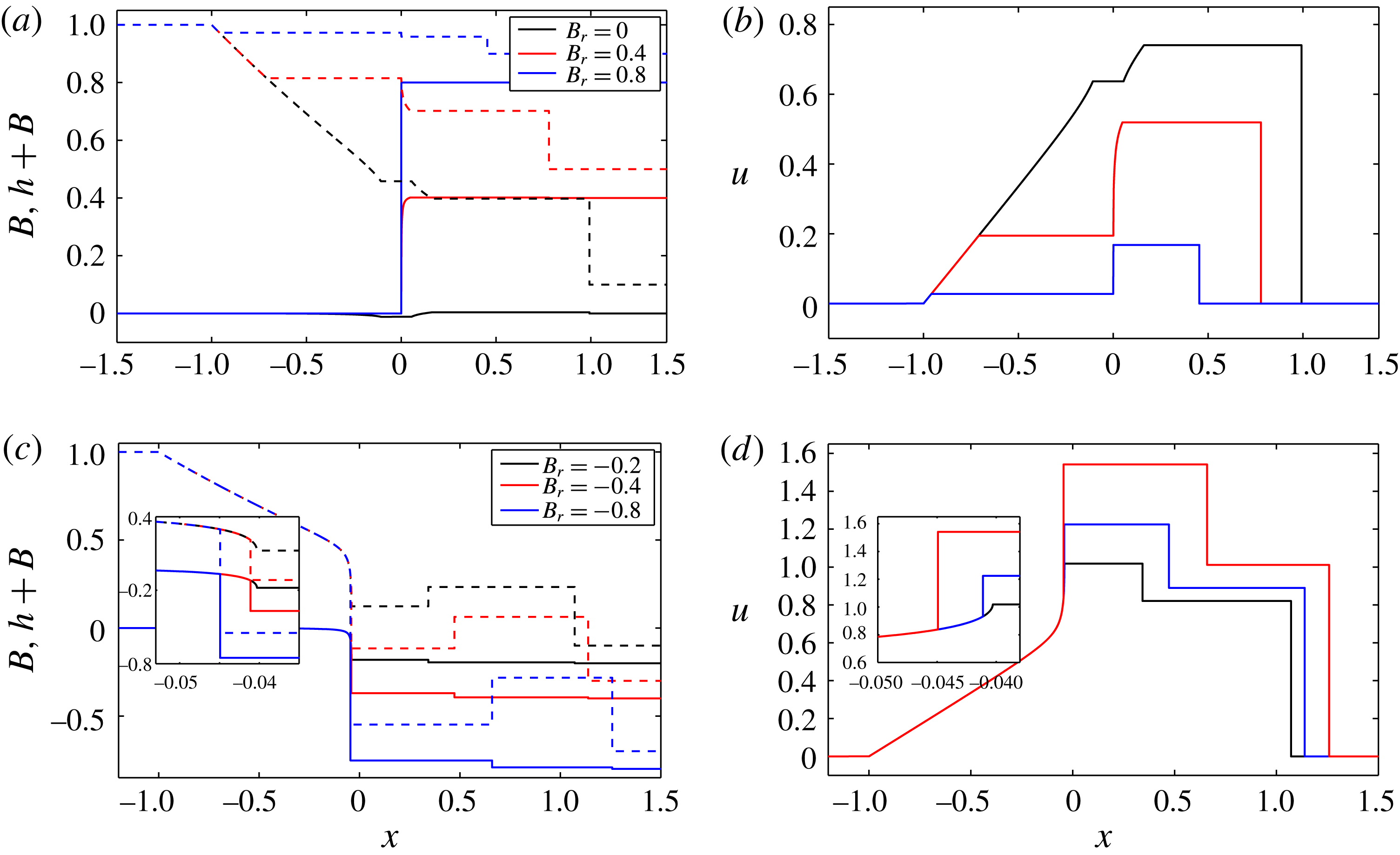
are shown in figure 6.
Structure of the wave solution for a wet–dry dam-break problem (
 $h_{l}=1$
,
 $u_{l}=0$
,
 $B_{l}=0$
,
 $h_{r}=0$
,
 $u_{r}=0$
and
 $\unicode[STIX]{x1D70E}=0.01$
) with varying
 $B_{r}$
values (
 $t=1$
). All semi-characteristic shocks are solved by the
 $n$
-step approach for (2.27)–(2.29) with
 $n=2$
.

3.2.1
$B_{r}\geqslant B_{l}$

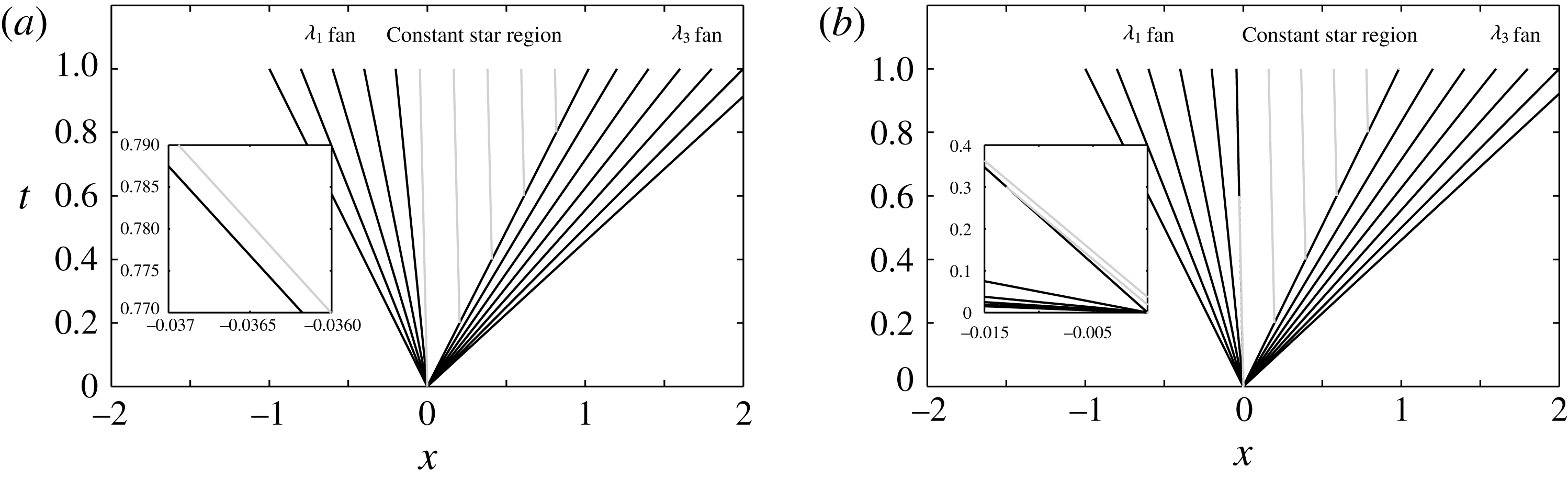
Figures 6(a) and 6(b) show, respectively, water surface elevation and bed level, and velocity. The wave structure is that of a
 $\unicode[STIX]{x1D706}_{1}$
rarefaction wave, a constant region,
 $\boldsymbol{U}_{\ast }$
, and a
 $\unicode[STIX]{x1D706}_{3}$
rarefaction wave, which is consistent with that presented by Kelly & Dodd (Reference Kelly and Dodd2009), who considered only
 $B_{r}=B_{l}=0$
. As
 $B_{r}\rightarrow B_{l}+h_{l}$
,
 $B_{\ast }+h_{\ast }\rightarrow B_{l}+h_{l}$
and the extents of the
 $\unicode[STIX]{x1D706}_{1}$
and
 $\unicode[STIX]{x1D706}_{3}$
rarefaction waves decrease, and the solution (at
 $t=1$
) resembles the initial conditions more. Note that the volume of water set in motion at time
 $t$
is
 $h_{l}|\unicode[STIX]{x1D706}_{1}(h_{l})|t$
, and is independent of
 $B_{r}$
because the left edge of the
 $\unicode[STIX]{x1D706}_{1}$
fan (
 $\unicode[STIX]{x1D706}_{1}(h_{l})$
) is unaffected by changes in
 $B_{r}$
. As the downstream elevation
 $B_{r}$
increases, velocities across the Riemann solution decrease, as, therefore, does the sediment movement. As
 $B_{r}$
increases, the flow in the constant region changes from supercritical (e.g. when
 $B_{r}=0$
) to subcritical flow (e.g. when
 $B_{r}=0.4$
or
 $0.8$
), and the
 $\unicode[STIX]{x1D706}_{3}$
wave close to
 $x=0$
changes from a hydrodynamic into a bed wave.
In the
 $\unicode[STIX]{x1D706}_{3}$
rarefaction fan,
 $$\begin{eqnarray}\displaystyle \text{d}B=\left(\frac{(\unicode[STIX]{x1D706}_{3}-u)^{2}}{h}-1\right)\,\text{d}h=-\frac{3\unicode[STIX]{x1D70E}u^{2}(\unicode[STIX]{x1D706}_{3}-u)}{\unicode[STIX]{x1D706}_{3}h}\,\text{d}h, & & \displaystyle\end{eqnarray}$$
where (2.11) has been used. Thus, the large bed change that occurs near the dam location for
 $B_{r}=0.4$
or
 $0.8$
is connected by the
 $\unicode[STIX]{x1D706}_{3}$
simple wave with
 $\unicode[STIX]{x1D706}_{3}\rightarrow 0$
in (3.1). The lip of the initial bed discontinuity is eroded by the flow, and the initial discontinuity in bed level is transformed into a steep continuous variation. The small bed step (Kelly & Dodd Reference Kelly and Dodd2010) at the flow tip (
 $x=x_{s}(t)$
) remains a feature of the solutions with decreasing height as flow velocity there decreases as
 $B_{r}$
increases. For
 $B_{r}=h_{l}+B_{l}$
no flow ensues, and there is no erosion.
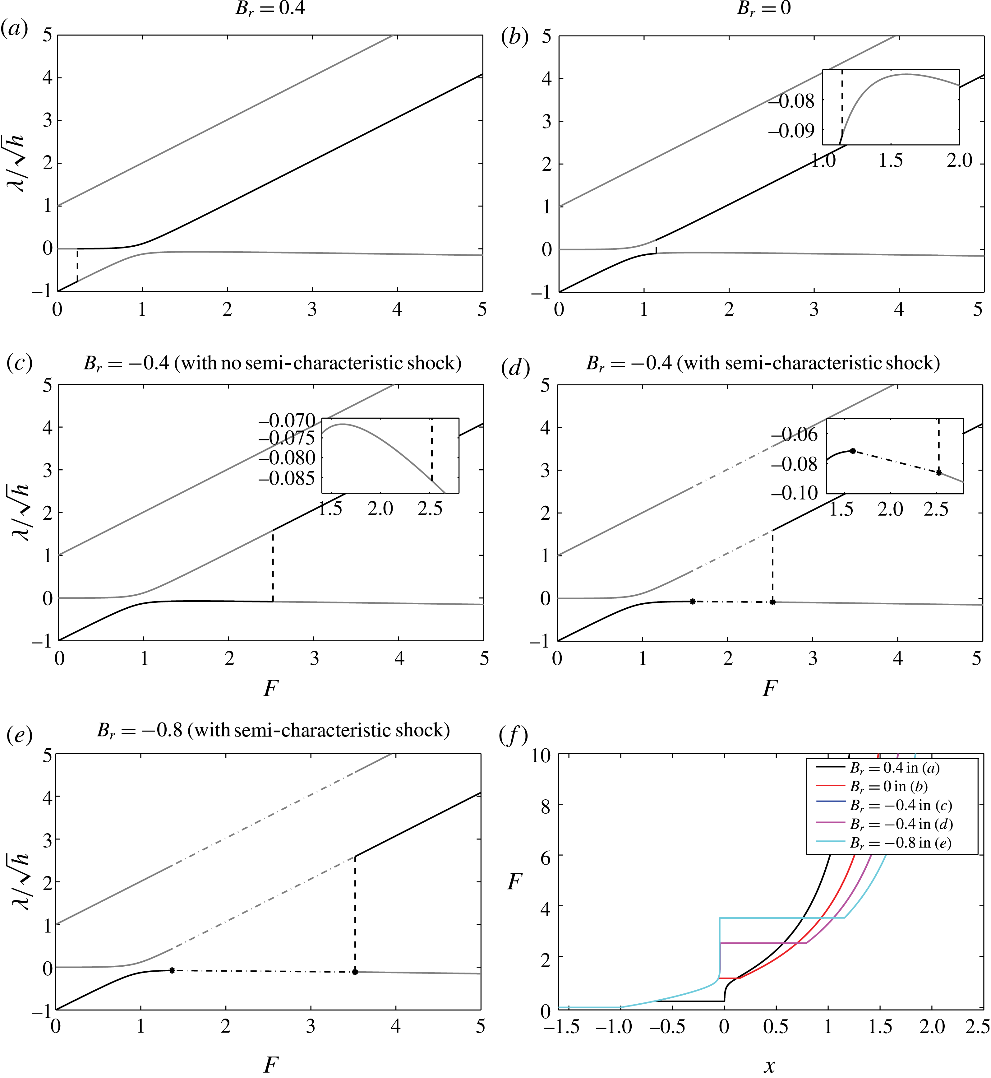
Illustrations of four of the Riemann solutions depicted in figure 6 in (
 $\unicode[STIX]{x1D706}/\sqrt{h},F$
) space as the solution is traversed from
 $x_{l}$
to
 $x_{s}$
. Dashed lines represent the jumps from
 $\unicode[STIX]{x1D706}_{1}$
wave and
 $\unicode[STIX]{x1D706}_{3}$
wave. Dash-dotted lines represent the jump at the semi-characteristic shocks. (f) Illustration of how
 $F$
varies across these solutions.

The wave development is closely related to Froude number (
 $F$
), and Froude number acts as a proxy for position
 $x$
. In figure 7(f), we show the relationship between
 $F$
and
 $x$
.
 $F$
increases across the Riemann solution as
 $x$
increases. In figure 7(a,b) the three derived characteristic velocities
 $\unicode[STIX]{x1D706}^{\prime }=\unicode[STIX]{x1D706}/\sqrt{h}$
are plotted as a function of Froude number (
 $F$
). Again, note that the
 $\unicode[STIX]{x1D706}^{\prime }$
curves are invariant for all dam-break solutions with
 $\unicode[STIX]{x1D70E}=0.01$
unless there is a discontinuity in
 $F$
when a shock develops. In contrast, the black line superimposed on parts of these curves indicates the variation of
 ${\unicode[STIX]{x1D706}^{\prime }}_{1}$
across the
 $\unicode[STIX]{x1D706}_{1}$
fan, and the variation of
 ${\unicode[STIX]{x1D706}^{\prime }}_{3}$
across the
 $\unicode[STIX]{x1D706}_{3}$
fan, with the jump from one to the other also depicted, for
 $B_{r}=0$
and
 $0.4$
. If we follow the (black)
 ${\unicode[STIX]{x1D706}^{\prime }}_{i}$
values along the
 ${\unicode[STIX]{x1D706}^{\prime }}_{i}$
curves in figure 7(a,b) from
 $F=0$
we see that
 ${\unicode[STIX]{x1D706}^{\prime }}_{1}$
increases as
 $F$
increases for
 $B_{r}=0.4$
and
 $0$
. For
 $B_{r}=0$
the jump from
 ${\unicode[STIX]{x1D706}^{\prime }}_{1}$
to
 ${\unicode[STIX]{x1D706}^{\prime }}_{3}$
for
 $B_{r}\geqslant 0$
, which corresponds to the constant region, occurs for a larger
 $F$
value than that for
 $B_{r}=0.4$
. Both jumps occur prior to the point at which
 $\text{d}{\unicode[STIX]{x1D706}^{\prime }}_{1}/\text{d}F=0$
. Therefore,
 $\unicode[STIX]{x1D706}^{\prime }$
increases monotonically across both fans.
 $(\text{d}{\unicode[STIX]{x1D706}^{\prime }}_{1}/\text{d}F)=0$
, indicating a convergence in
 ${\unicode[STIX]{x1D706}^{\prime }}_{1}$
, occurs at
 $F\approx 1.6$
for all dam-break solutions with
 $\unicode[STIX]{x1D70E}=0.01$
.
3.2.2
$B_{r}\leqslant B_{l}$

In figure 6(c,d) we can see the dam-break structure in this case, which is similar to the preceding one in that two rarefaction fans (
 $\unicode[STIX]{x1D706}_{1}$
and
 $\unicode[STIX]{x1D706}_{3}$
) form, separated by a constant region.
Before commenting further on the structure of these solutions it is instructive first to consider their representation in (
 $\unicode[STIX]{x1D706}^{\prime },F$
) space. In figure 7(c–e) we do this. Figure 7(c,d) illustrates the behaviour for
 $B_{r}=-0.4$
. For figure 7(c) we see the elementary wave solution. Note, however, that the jump via the constant region, from
 ${\unicode[STIX]{x1D706}^{\prime }}_{1}$
to
 ${\unicode[STIX]{x1D706}^{\prime }}_{3}$
curve, occurs when
 $(\text{d}{\unicode[STIX]{x1D706}^{\prime }}_{1}/\text{d}F)<0$
. This implies that at some point within the
 $\unicode[STIX]{x1D706}_{1}$
fan the
 ${\unicode[STIX]{x1D706}^{\prime }}_{1}$
derived characteristics start decreasing as
 $F$
increases. In contrast figure 7(d) shows the behaviour with a semi-characteristic shock included.
Representing the solution in (
 $\unicode[STIX]{x1D706}^{\prime },F$
) space is appealing because these curves are invariant with the continuous Riemann solution (i.e. size of bed step). However, it is the convergence of
 $\unicode[STIX]{x1D706}_{1}$
characteristics (not
 ${\unicode[STIX]{x1D706}^{\prime }}_{1}$
) in the
 $(x,t)$
-plane that determines whether or not a semi-characteristic shock must be fitted. So, to determine this point of change in the Riemann solution it is appropriate to examine variation in
 $\unicode[STIX]{x1D706}_{1}$
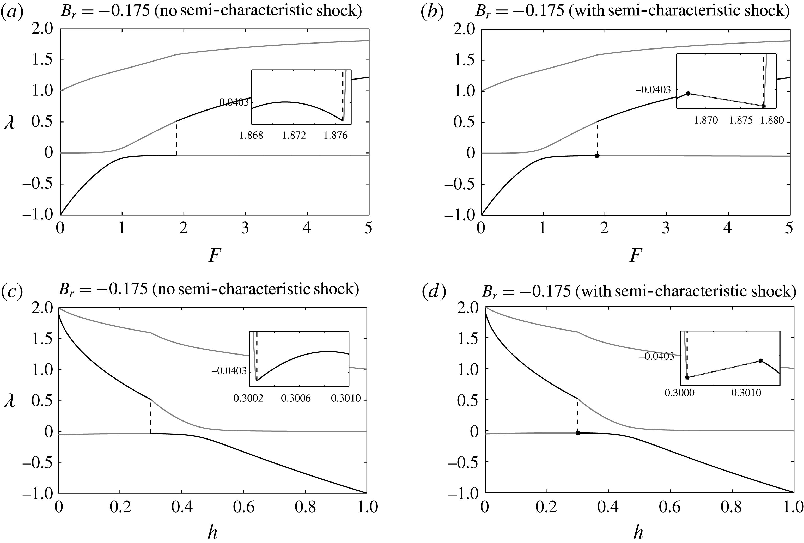
. The multivalued solution of
 $\unicode[STIX]{x1D706}_{1}$
starts at
 $B_{r}\lessapprox -0.175$
, at the location at which
 $F\approx 1.87$
(and
 $h\approx 0.301$
). This point is illustrated in figure 8.
 $\unicode[STIX]{x1D706}_{1}$
increases as
 $F$
increases, but at
 $F\approx 1.87$
the characteristic velocity (
 $\unicode[STIX]{x1D706}_{1}$
) starts to decrease at the leading edge of the
 $\unicode[STIX]{x1D706}_{1}$
rarefaction fan. The constant region, corresponding to the jump from
 $\unicode[STIX]{x1D706}_{1}$
to
 $\unicode[STIX]{x1D706}_{3}$
curve, thus occurs when
 $(\text{d}\unicode[STIX]{x1D706}_{1}/\text{d}F)<0$
. This indicates the convergence of
 $\unicode[STIX]{x1D706}_{1}$
characteristics within the
 $\unicode[STIX]{x1D706}_{1}$
fan. The solution is multivalued. The part of the
 $\unicode[STIX]{x1D706}_{1}$
curve for which
 $F>1$
behaves like a characteristic associated with a bed wave. Because
 $\unicode[STIX]{x1D706}_{1}<0$
this behaviour results in a bed wave propagating against the flow. Similar behaviour can be observed in the propagation of anti-dunes in supercritical open channel flow on a mobile bed, which propagate against the flow (see Kennedy Reference Kennedy1963).
Illustrations of Riemann solutions for dam-break problems with
 $h_{l}=1$
,
 $u_{l}=0$
,
 $B_{l}=0$
,
 $h_{r}=0$
,
 $u_{r}=0$
,
 $B_{r}=0.175$
and
 $\unicode[STIX]{x1D70E}=0.01$
in (
 $\unicode[STIX]{x1D706},F$
) and (
 $\unicode[STIX]{x1D706},h$
) space to indicate why a semi-characteristic shock must be fitted. Dashed lines represent the jumps from
 $\unicode[STIX]{x1D706}_{1}$
wave and
 $\unicode[STIX]{x1D706}_{3}$
wave. Dash-dotted lines represent the jump at the semi-characteristic shocks. All semi-characteristic shocks are solved by the
 $n$
-step approach for (2.27)–(2.29) with
 $n=2$
.

To obtain a valid mathematical structure here, the
 $\unicode[STIX]{x1D706}_{1}$
fan must terminate prior to the point at which
 $(\text{d}\unicode[STIX]{x1D706}_{1}/\text{d}h)=0$
at a semi-characteristic shock with
 ${\unicode[STIX]{x1D706}_{1}}_{L}=W$
; downstream, in the constant region we must have
 ${\unicode[STIX]{x1D706}_{1}}_{R}<W$
, for a valid shock structure, which is possible because
 $F$
increases across the shock and therefore
 $\unicode[STIX]{x1D706}_{1}$
decreases.
Physically, the main difference between this case and that for
 $B_{r}>B_{l}$
is the larger velocities induced by the lower downstream elevation, which drives the early supercritical flow development and therefore the formation of the semi-characteristic shock. Now, the constant region is shifted mostly to
 $x>0$
, with a large decrease in
 $h_{\ast }$
. The flow is supercritical at the dam location, and the
 $\unicode[STIX]{x1D706}_{1}$
wave has become a bed wave close to
 $x=0$
, where we can also see the large bed change. The large bed decrease occurs at the shock, which helps to connect widely separated values of
 $B_{l}$
and
 $B_{r}$
.
We assume an implied internal shock structure for all the semi-characteristic shocks, and
 $n=2$
is adopted here. For the semi-characteristic shocks for all negative
 $B_{r}$
values, we have
 $\unicode[STIX]{x1D706}_{1L}=W>\unicode[STIX]{x1D706}_{1R}$
. The convergence of characteristics implies that the shocks are physical. Note that if we use the approximation (2.30) we do not arrive at physical solutions for
 $B_{r}=-0.8$
, and if we use the approximation (2.31) we do not get solutions for any semi-characteristic shocks with the examined
 $B_{r}$
values. It is therefore critical that we introduce this more accurate approach. In appendix C we show the equivalent solutions and examine dependence on
 $n$
.
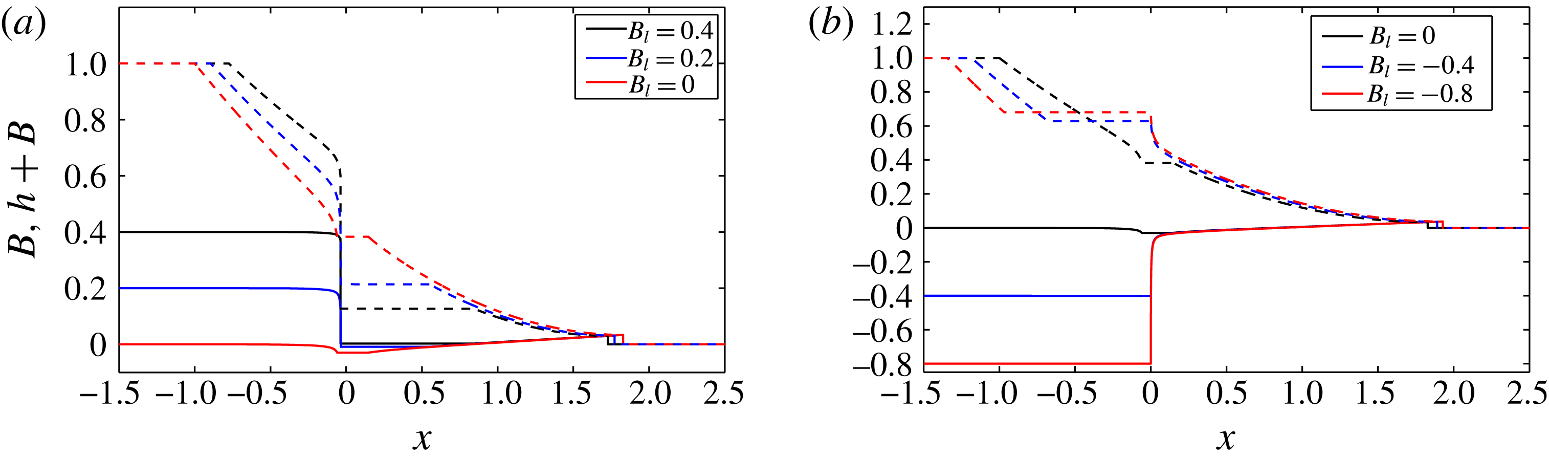
3.2.3 Varying upstream bed level
We also examine the effect of varying the upstream bed level only, while keeping the upstream surface elevation and downstream bed level fixed (
 $h_{l}+B_{l}=1$
and
 $B_{r}=0$
). The Riemann solutions (
 $B$
and
 $B+h$
only) are shown in figure 9. The structures are similar to those already observed, but now with particularly large variations between solutions for
 $x<0$
, because
 $h_{l}$
varies and so therefore does the driving force.


The wave solutions of these dam-break problems are similar to those of fixed
 $h_{l}$
and
 $B_{l}$
values (
 $h_{l}=1$
,
 $B_{l}=0$
) but varying
 $B_{r}$
values. Actually, these two kinds of dam-break problems can be converted to each other through scaling and transformation. It is the water depth on the left and bed difference that determines the wave structure. Two dam-break problems with the same ratios of water depths and bed differences, i.e.
 $h_{l1}/h_{l2}=(B_{l1}-B_{r1})/(B_{l2}-B_{r2})$
are similar. Therefore the wave structures after dam collapse are similar.
3.3 Wet–wet dam-break problem
We now turn to the wet–wet dam-break solution over an initially piecewise flat erodible bed for various
 $B_{r}$
values, which consists of elementary waves. The solutions at
 $t=1$
are shown in figure 10.
3.3.1
$B_{r}\geqslant B_{l}$

Figure 10(a,b) shows, respectively, water surface level and bed level, and velocity for this case. The wave structure is of a
 $\unicode[STIX]{x1D706}_{1}$
rarefaction wave, a
 $\unicode[STIX]{x1D706}_{3}$
rarefaction wave and a
 $\unicode[STIX]{x1D706}_{2}$
shock. There are two newly formed constant regions (
 $\boldsymbol{U}_{l\ast }$
and
 $\boldsymbol{U}_{r\ast }$
) separating the three waves. For
 $B_{r}=0$
, the
 $\unicode[STIX]{x1D706}_{2}$
shock corresponds to the
 $\unicode[STIX]{x1D706}_{+}$
shock in the equivalent fixed-bed wet–wet dam-break problem (e.g. Toro Reference Toro2001), and the
 $\unicode[STIX]{x1D706}_{1}$
and
 $\unicode[STIX]{x1D706}_{3}$
rarefaction waves correspond to the
 $\unicode[STIX]{x1D706}_{-}$
rarefaction wave in the fixed-bed case. When the bed mobility
 $\unicode[STIX]{x1D70E}\rightarrow 0$
, the
 $\unicode[STIX]{x1D706}_{1}$
and
 $\unicode[STIX]{x1D706}_{3}$
rarefaction waves tend to combine into one wave.
As
 $B_{r}$
increases, the
 $\unicode[STIX]{x1D706}_{3}$
wave becomes more confined to the original bed step position, and less water flows into
 $x>0$
region. When
 $h_{r}+B_{r}\rightarrow 1$
flow ceases.
Structure of the wave solution for a wet–wet dam-break problem (
 $h_{l}=1$
,
 $u_{l}=0$
,
 $B_{l}=0$
,
 $h_{r}=0.1$
,
 $u_{r}=0$
and
 $\unicode[STIX]{x1D70E}=0.01$
) with varying
 $B_{r}$
values at
 $t=1$
. All semi-characteristic shocks are solved by the
 $n$
-step approach for (2.27)–(2.29) with
 $n=2$
.

3.3.2
$B_{r}\leqslant B_{l}$

In figure 10(c,d), we can see the dam-break structure in this case. There is still a
 $\unicode[STIX]{x1D706}_{1}$
rarefaction wave, and a
 $\unicode[STIX]{x1D706}_{2}$
shock, as for
 $B_{r}>B_{l}$
. However, for the investigated negative
 $B_{r}$
values, the
 $\unicode[STIX]{x1D706}_{3}$
wave changes from a rarefaction wave into a shock. There are also two newly formed constant regions. For
 $B_{r}<0$
as
 $B_{r}$
decreases further (see figure 10
c),
 $h_{l\ast }$
decreases very quickly, and when
 $h_{l\ast }<h_{r\ast }$
the
 $\unicode[STIX]{x1D706}_{3}$
fan observable for
 $B_{r}=0$
becomes a shock as the characteristics converge.
When
 $B_{r}\lessapprox -0.207$
, we get multivalued solutions within the
 $\unicode[STIX]{x1D706}_{1}$
fan, (see figure 10
c). The
 $B_{r}$
value at which this occurs will depend on
 $h_{r}$
, which here is
 $0.1$
. We again assume the existence of a
 $\unicode[STIX]{x1D706}_{1}$
semi-characteristic shock, and the corresponding wave structure is shown in figure 10(c,d). Once again, we assume an implied internal shock structure, expressed through (2.34) in (2.27)–(2.29), in order to obtain a physical shock (see appendix C).
3.3.3 Varying downstream water depth
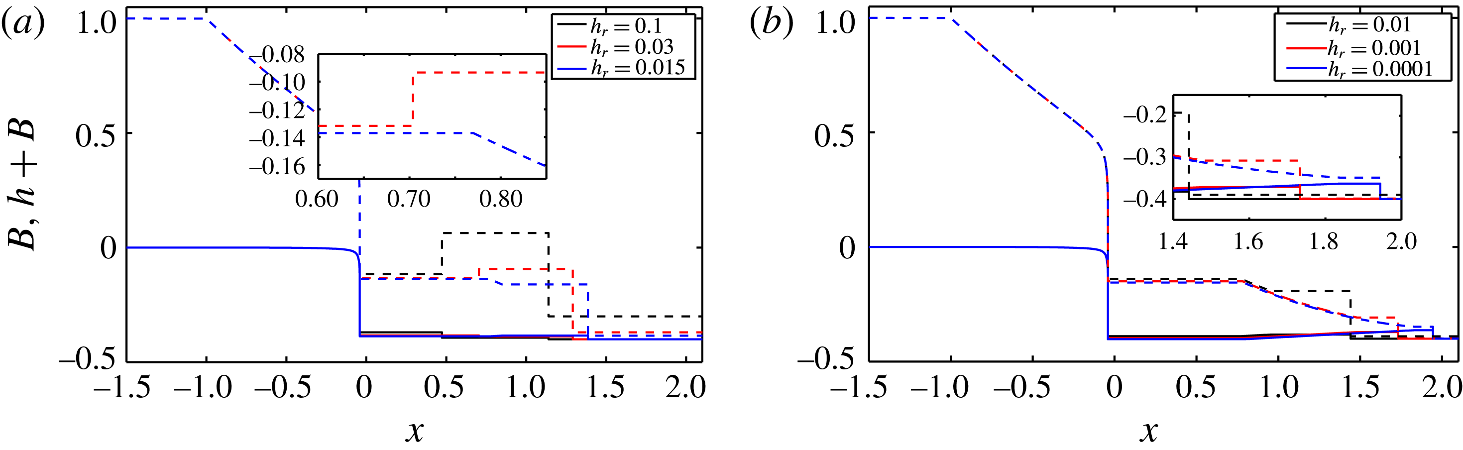
In figure 11 we look at the effect that varying
 $h_{r}$
has on the structure of these problems. As
 $h_{r}$
decreases, we expect this wet–wet problem to start to resemble previously examined wet–dry problems (see figure 6). Accordingly, the
 $\unicode[STIX]{x1D706}_{3}$
shock diminishes such that between
 $h_{r}=0.03$
and
 $0.015$
it becomes a rarefaction fan. As
 $h_{r}$
decreases further the
 $\unicode[STIX]{x1D706}_{3}$
fan extends towards the
 $\unicode[STIX]{x1D706}_{2}$
shock such that in the limit
 $h_{r}\rightarrow 0$
the leading edge of this
 $\unicode[STIX]{x1D706}_{3}$
fan becomes the wet–dry boundary (with zero depth) and a semi-characteristic shock, and the
 $\unicode[STIX]{x1D706}_{2}$
shock disappears. The
 $\unicode[STIX]{x1D706}_{1}$
wave is a combination of a fan and a semi-characteristic shock, which is consistent with the equivalent wet–dry dam-break solution.
Structure of the wave solution for a wet–wet Riemann problem with (
 $h_{l}=1$
,
 $u_{l}=0$
,
 $B_{l}=0$
,
 $u_{r}=0$
,
 $B_{r}=-0.4$
and
 $\unicode[STIX]{x1D70E}=0.01$
) varying
 $h_{r}$
values.

4 Conclusion
Generalised wet–dry and wet–wet dam-break problems over an erodible, initially piecewise flat bed with water initially at rest and discontinuous bed levels are investigated and solved based on the Riemann theory, and quasi-exact solutions are presented. The solutions are consistent with the theory proposed by Lax (Reference Lax1973) that for a Riemann problem of
 $n$
equations there are at most
 $n+1$
constant states separated by
 $n$
elementary waves associated with the
 $n$
characteristic families. However, for wet–dry dam-break problems, one wave vanishes because of the presence of the dry bed. For the examined wet–dry dam-break problems, there are two waves separated by one newly formed constant region, which is in agreement with that in Kelly & Dodd (Reference Kelly and Dodd2009).
For some dam-break problems with negative bed steps, in which the initial states (
 $B_{l}$
and
 $B_{r}$
) are not sufficiently close, there are multivalued solutions when applying Lax’s theorem. The semi-characteristic shock is introduced to describe the flow and physical wave structures are obtained. This is consistent with the solution for a Riemann problem of one single equation of non-convex flux function (Sharma Reference Sharma2010).
The ambiguous integral
 $\int _{x_{L}}^{x_{R}}hB_{x}\,\text{d}x$
in shock conditions, which is usually approximated by the Needham & Hey (Reference Needham and Hey1991) approach, is reconsidered. An implied internal shock structure is proposed initially by considering the limiting case of flow down a linear slope over fixed bed. Based on the internal shock structure, the integral
 $\int _{x_{L}}^{x_{R}}hB_{x}\,\text{d}x$
is discretised into many steps and each step is approximated by the Needham & Hey (Reference Needham and Hey1991) approach. This is to reduce the effects of curvature between
 $h$
and
 $B$
, which is source of inaccuracy in the Needham & Hey (Reference Needham and Hey1991) approximation. This strategy is then extended to morphodynamic shocks which are here by assumption slow moving. However, because of the more general implied internal shock structure approach we ultimately adopt it would appear that this approach is more generally applicable. The resulting semi-characteristic shocks are physical, in that the characteristics converge across them.
Acknowledgements
F.Z. and N.D. would like to acknowledge the financial support from both National Natural Science Foundation of China (grant no. 51509135) and University of Nottingham Ningbo China (Small Research Grant). The authors would also like to thank the anonymous reviewers for their constructive comments.
Appendix A. Analysis of
$\int _{\tilde{B}_{L}}^{\tilde{B}_{R}}\tilde{h}\,\text{d}\tilde{B}$
approximation methods

In this section, we analyse the performances of three approximation methods for the ambiguous term
 $\int _{\tilde{B}_{L}}^{\tilde{B}_{R}}\tilde{h}\,\text{d}\tilde{B}$
(in the original non-dimensional system
 $\int _{B_{L}}^{B_{R}}h\,\text{d}B$
in shock condition (2.28)) on a linear (fixed) slope in § 2.7: (2.30), (2.31) and (2.34) with (2.40) against the exact solution (2.41) with (2.40).
Here, we take
 $\tilde{B}_{L}=0$
and
 $\tilde{B}_{R}=-\tilde{x}$
, with
 $\tilde{x}>0$
being a variable. The approximation (2.30) gives
 $$\begin{eqnarray}\int _{0}^{-\tilde{x}}\tilde{h}\,\text{d}\tilde{B}=-\frac{1}{2}\tilde{x}(1+\tilde{h}),\end{eqnarray}$$
and it is exact if the relationship between
 $\tilde{h}$
and
 $\tilde{B}$
is linear. The approximation (2.31) is
 $$\begin{eqnarray}\displaystyle \int _{0}^{-\tilde{x}}\tilde{h}\,\text{d}\tilde{B}=\left\{\begin{array}{@{}ll@{}}-{\displaystyle \frac{1}{2}}\tilde{x}(2\tilde{h}-\tilde{x})\quad & \text{if }\tilde{B}_{R}<\tilde{B}_{L}\text{ and }\tilde{B}_{R}+\tilde{h}_{R}>\tilde{B}_{L},\\ -{\displaystyle \frac{1}{2}}\tilde{h}^{2}\quad & \text{if }\tilde{B}_{R}+\tilde{h}_{R}<\tilde{B}_{L}.\end{array}\right. & & \displaystyle\end{eqnarray}$$
We also use the
 $n$
-step approach (2.34) with
 $n=5$
for the approximation
 $$\begin{eqnarray}\displaystyle \int _{0}^{-\tilde{x}}\tilde{h}\,\text{d}\tilde{B} & = & \displaystyle -\frac{1}{2}\mathop{\sum }_{i=0}^{i=4}(\tilde{h}_{i}+\tilde{h}_{i+1})(\tilde{B}_{i+1}-\tilde{B}_{i}),\end{eqnarray}$$
with
 $\tilde{B}_{i}=-\text{i}\tilde{x}/5$
, in which
 $h_{i}$
is calculated by (2.40).
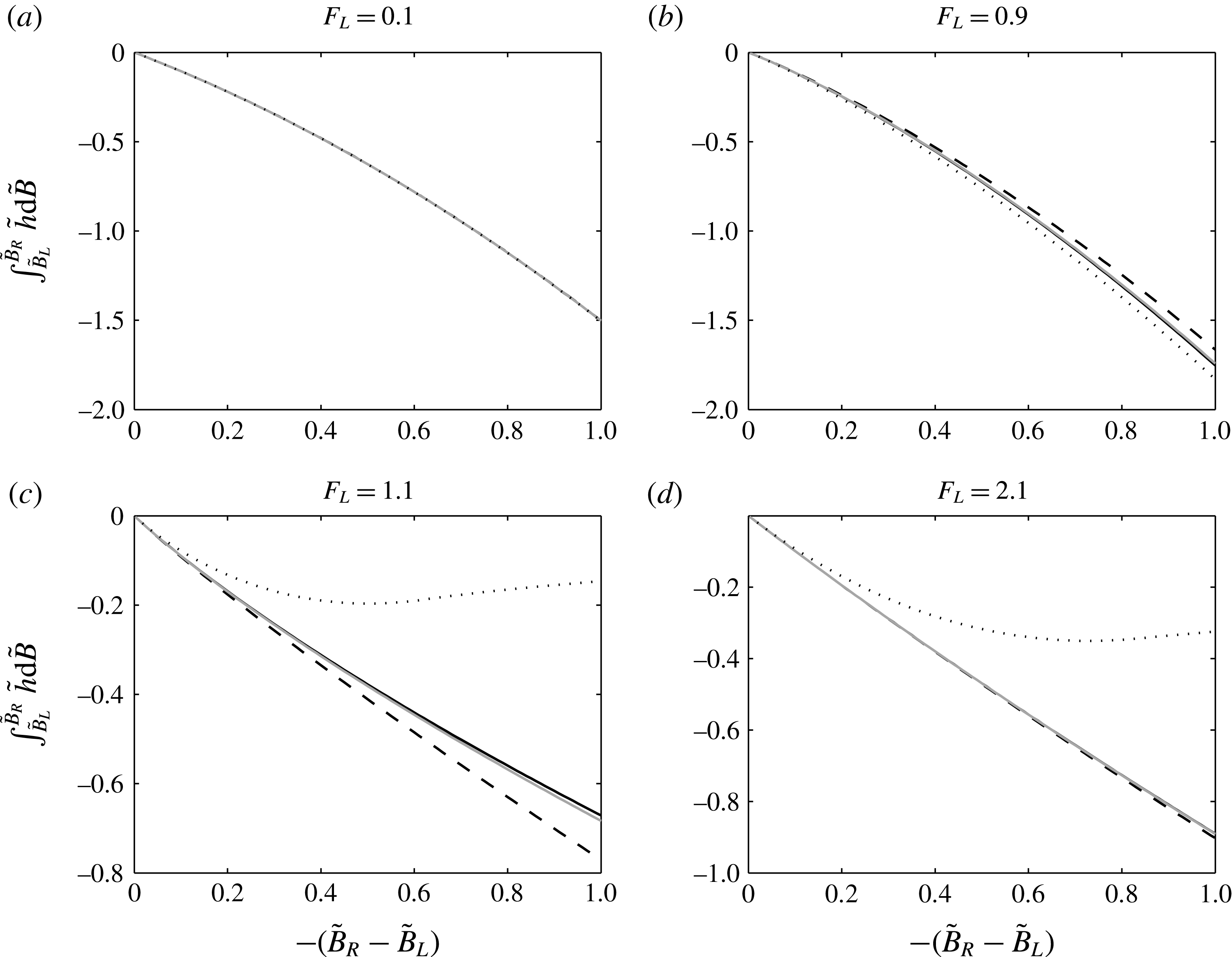
The results of (A 1), (A 2), (A 3) and (2.41) are illustrated in figure 12. Comparison shows that the approximation (A 1), i.e. (2.30), is generally quite accurate. Nearer to critical conditions the free surface curvature introduces significant discrepancies. Also, as
 $\tilde{B}_{R}-\tilde{B}_{L}$
increases, accuracy diminishes. The
 $n$
-step approach (A 3), i.e. (2.34), greatly increases the accuracy. The approximation (A 2), i.e. (2.31) (Bernetti et al.
Reference Bernetti, Titarev and Toro2008), is indistinguishable from the exact value when it is subcritical flow. It slightly overestimates the exact value when it is closer to critical flow. However, when the flow is supercritical, the discrepancies become significant.
 $\int _{\tilde{B}_{L}}^{\tilde{B}_{R}}\tilde{h}\,\text{d}\tilde{B}$
plotted against size of bed step:
 $\int _{\tilde{B}_{L}}^{\tilde{B}_{R}}\tilde{h}\,\text{d}\tilde{B}=-[F_{L}^{2}(1/\tilde{h})+(1/2)\tilde{h}^{2}]_{L}^{R}$
calculated using (2.40) (solid black line); that approximated by (A 1), i.e. (2.30) (dashed line), by (A 2), i.e. (2.31) (dotted line) and by (A 3), i.e. (2.34) with
 $n=5$
(grey solid line) for various Froude numbers.

Appendix B. Comparison between wet–dry dam-break Riemann solution of fixed and nearly fixed-bed case
In this section, we test the Riemann solver by comparing the nearly fixed-bed wet–dry dam-break solution (
 $\unicode[STIX]{x1D70E}=1\times 10^{-5}$
) against the fixed-bed solution.
The dam-break problem over a fixed bed with a bed step will lead to a stationary shock at the bed step (Bernetti et al.
Reference Bernetti, Titarev and Toro2008). For the positive
 $B_{r}$
values examined, the wave structure over a fixed bed from the left to right is a
 $\unicode[STIX]{x1D706}_{-}$
rarefaction wave, a constant region, a stationary shock and a
 $\unicode[STIX]{x1D706}_{-}$
rarefaction wave. That for the negative
 $B_{r}$
values examined is a
 $\unicode[STIX]{x1D706}_{-}$
rarefaction wave, a stationary shock, a constant region and a
 $\unicode[STIX]{x1D706}_{-}$
rarefaction wave (figure 13). This stationary shock corresponds to a semi-characteristic shock if we interpret it in a morphodynamic context. It is a
 $\unicode[STIX]{x1D706}_{3}$
semi-characteristic shock with
 $\unicode[STIX]{x1D706}_{3L}=W=\unicode[STIX]{x1D706}_{3R}=0$
because
 $\unicode[STIX]{x1D70E}=0$
.
Comparison between wet–dry dam-break fixed bed (
 $h_{l}=1$
,
 $u_{l}=0$
,
 $B_{l}=0$
,
 $h_{r}=0$
,
 $u_{r}=0$
and
 $B_{r}=0$
) solution (
 $\unicode[STIX]{x1D70E}=0$
; solid lines) and nearly fixed-bed solution (
 $\unicode[STIX]{x1D70E}=1\times 10^{-5}$
; dashed lines). All semi-characteristic shocks are solved with the NH91 approximation.

On a nearly fixed bed, the wave structure for the non-negative
 $B_{r}$
values examined, is a
 $\unicode[STIX]{x1D706}_{1}$
rarefaction wave, a constant region and a
 $\unicode[STIX]{x1D706}_{3}$
rarefaction wave. The stationary shock in the fixed-bed case disappears because of the bed mobility, and the left part of the
 $\unicode[STIX]{x1D706}_{3}$
rarefaction wave becomes a steep but smooth part, which is to some extent similar to the stationary shock in the fixed-bed case. The nearly fixed-bed solutions are in good agreement with the fixed-bed solutions (figure 13
a).
The Riemann solutions with the NH91 condition for the examined negative
 $B_{r}$
values over a nearly fixed bed are similar to those presented in § 3.2.2. The wave structures are a
 $\unicode[STIX]{x1D706}_{1}$
rarefaction, a
 $\unicode[STIX]{x1D706}_{1}$
semi-characteristic shock and a
 $\unicode[STIX]{x1D706}_{3}$
rarefaction. The
 $\unicode[STIX]{x1D706}_{1}$
rarefaction fan corresponds to the stationary shock on the fixed bed. The results compare favourably with the corresponding fixed-bed results (figure 13
b).
Appendix C. Investigation of
$\int _{B_{L}}^{B_{R}}h\,\text{d}B$
approximation methods in dam-break problems

In this section, we investigate the approximation of
 $\int _{B_{L}}^{B_{R}}h\,\text{d}B$
by comparing the solutions of wet–dry and wet–wet dam-break problems using different approximation methods (see appendix A and § 2.7.2). In summary, the approximation methods include (a): (2.41) together with (2.40) and (2.29), i.e.
 $h_{R}$
and
 $u_{R}$
are directly calculated for a known
 $B_{R}$
as for the stationary shock across a fixed-bed discontinuity; (b):
 $n$
-step approach with (2.40) applied in (2.43), (2.44) and (2.29) (c):
 $n$
-step approach with (2.27)–(2.28) for
 $h_{i}$
,
 $u_{i}$
and
 $B_{i}$
for (2.27)–(2.29), (d): NH91 approximation (i.e.
 $n$
-step approach in method (c) with
 $n=1$
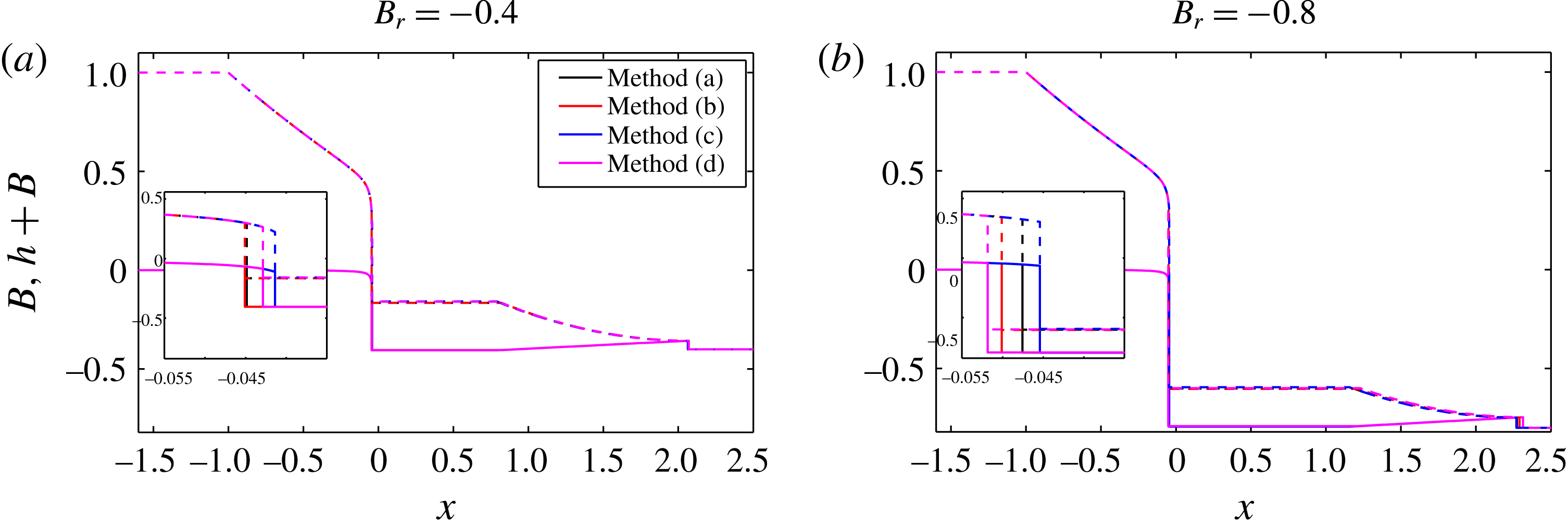
); and (e): Bernetti et al. (Reference Bernetti, Titarev and Toro2008) condition for (2.27)–(2.29). It should be noted that with the Bernetti et al. (Reference Bernetti, Titarev and Toro2008) condition, we cannot find a solution if a semi-characteristic shock is assumed, i.e. there is no alternative to the multivalued solution.
The performances of the approximation methods for
 $\int _{B_{L}}^{B_{R}}h\,\text{d}B$
are compared by examining wet–dry dam-break solutions for both
 $B_{r}=-0.4$
and
 $-0.8$
. In general, the approximations give similar results for water levels and bed elevations when the whole solution is shown. Differences can be seen at the semi-characteristic shock. When
 $B_{r}=-0.4$
, method (a) and (b) give very similar results, and the results of method (c) and (d) are close. When the bed step height increases, the difference grows. However, the semi-characteristic shocks predicted by method (a) and (b) for
 $B_{r}=-0.4$
(and
 $B_{r}=-0.2$
, not shown) and that by method (d) for
 $B_{r}=-0.8$
(and
 $B_{r}=-0.6$
, not shown) are non-physical because
 $\unicode[STIX]{x1D706}_{1L}\geqslant W\geqslant \unicode[STIX]{x1D706}_{1R}$
cannot be satisfied. In contrast, method (c), used throughout this paper, results in a physical semi-characteristic shock for all these
 $B_{r}$
values. It is therefore necessary to retain the
 $W$
terms in (2.27)–(2.29).
The comparison of wet–dry dam-break (
 $h_{L}=1$
,
 $u_{L}=0$
,
 $B_{L}=0$
) solutions with different approximation methods for
 $\int _{B_{L}}^{B_{R}}h\,\text{d}B$
. In the
 $n$
-step approach in method (b) and (c),
 $n=2$
.

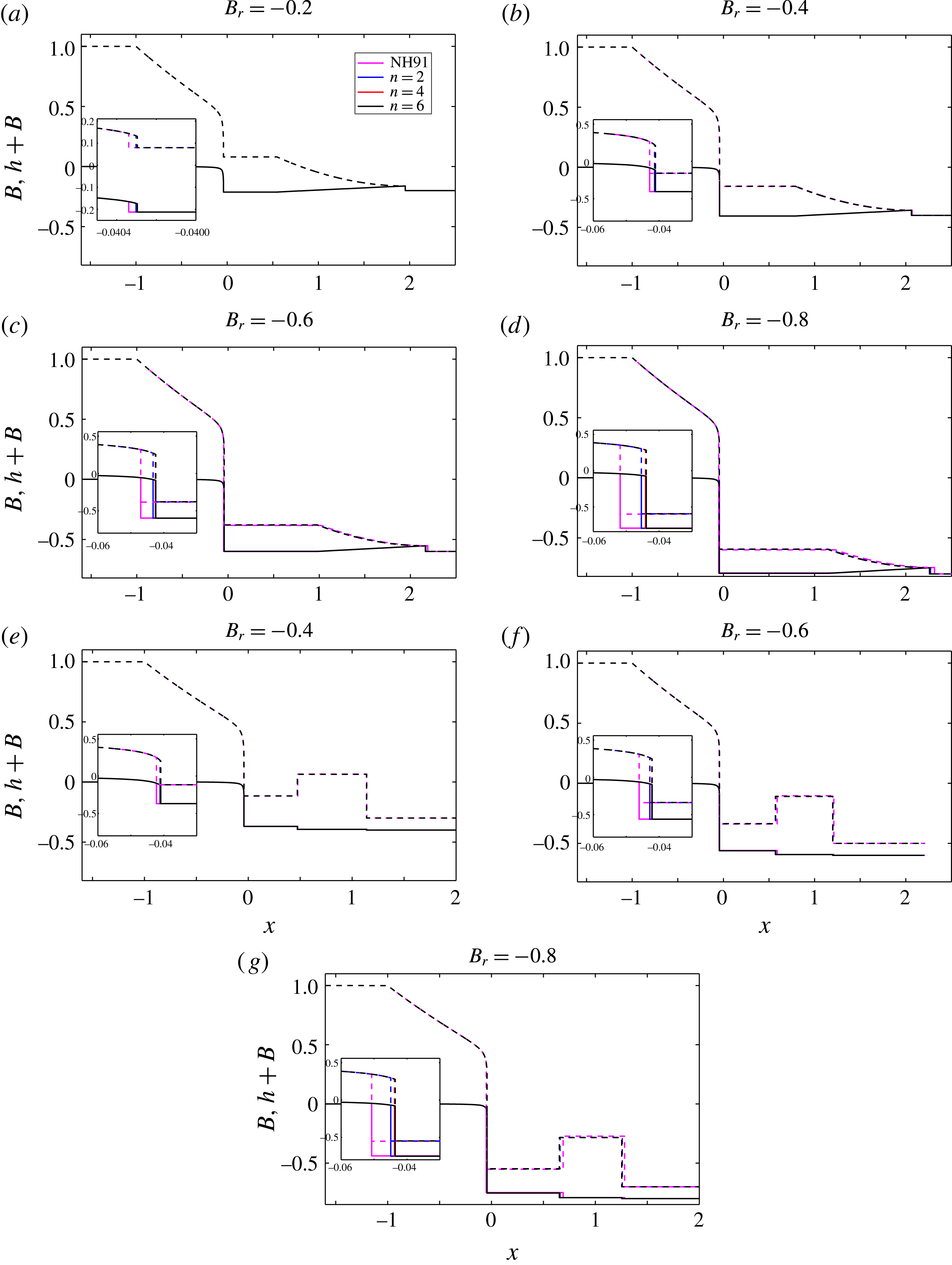
The effects of how many steps the integral
 $\int _{B_{L}}^{B_{R}}h\,\text{d}B$
is discretised into are also investigated. The comparison for both wet–dry and wet–wet dam-break problems using method (c) (
 $n$
-step approach) and (d) (NH91 approximation) is shown in figure 15. We can see that the results with the implied internal shock structure are initially very close to those directly using the NH91 approximation. As the size of bed step increases, the difference between solutions with the NH91 approximation and the new approach also increases slightly.
The comparison of dam-break solutions with the NH91 approximation and those with the implied internal shock structure (
 $n$
-step approach, for various
 $n$
values): (a–d) wet–dry dam-break solutions; (e–g) wet–wet dam-break solutions.

In the wet–dry dam-break problems with
 $B_{r}=-0.2,-0.4$
, the semi-characteristic shocks have
 $\unicode[STIX]{x1D706}_{1L}=W>\unicode[STIX]{x1D706}_{1R}$
when solved directly with the NH91 approximation. However, as previously mentioned, for
 $B_{r}=-0.6,-0.8$
, we have
 $\unicode[STIX]{x1D706}_{1L}=W<\unicode[STIX]{x1D706}_{1R}$
, which indicates a non-physical shock. It is further noted that in the
 $B_{r}=-0.4,-0.6,-0.8$
cases, the water on the left and right sides of the
 $\unicode[STIX]{x1D706}_{1}$
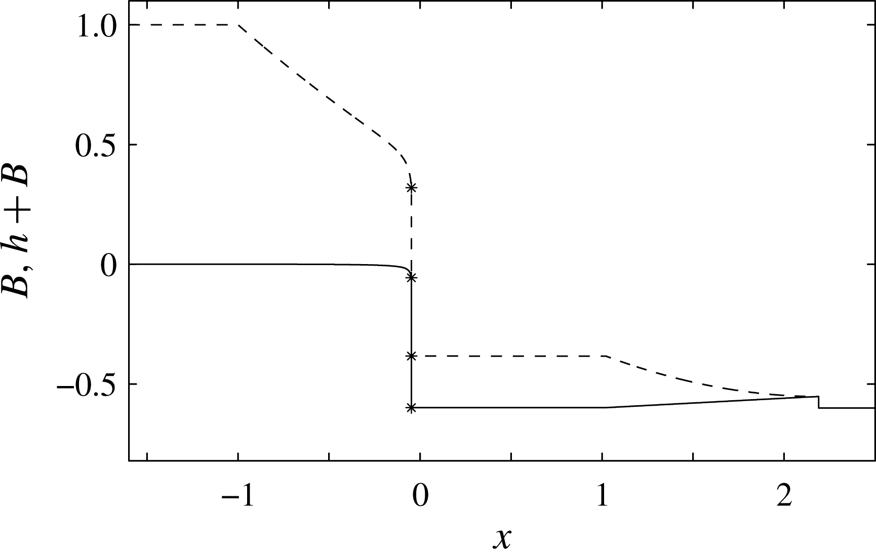
semi-characteristic shock are separated by the high bed step (figure 16). Similarly, in the wet–wet dam-break problems with
 $B_{r}=-0.6,-0.8$
, the semi-characteristic shocks are also non-physical. However, when we use the implied internal shock structure, the shocks become physical.
Structure of the wave solution (NH91 approximation) for a wet–dry dam-break problem with
 $B_{r}=-0.6$
which shows that the water on the two sides of the semi-characteristic shock is separated by the high bed step (
 $t=1$
).

In order to further investigate this, we take the wet–dry dam-break problem with
 $B_{r}=-0.6$
as an example to illustrate the characteristics across the semi-characteristic shocks; see figure 17. We can see the characteristics diverging when using the NH91 approximation, and characteristics converging when using implied internal shock structure. This indicates that the NH91 approximation becomes less accurate when the bed step becomes large in which case the curvature of
 $h$
with
 $B$
becomes enhanced. In this case, the importance of considering the internal shock structure becomes obvious.


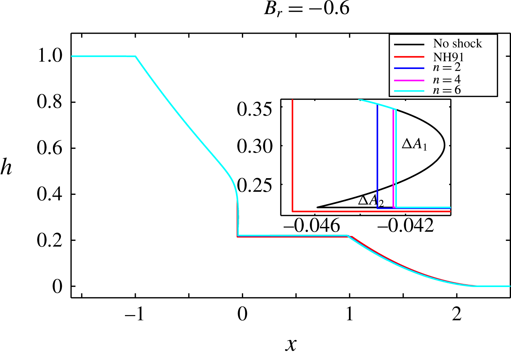
In figure 18 we see how the multivalued problem in a wet–dry dam-break problem is rationalised by introducing a semi-characteristic shock. According to Whitham (Reference Whitham1974), the areas
 $\unicode[STIX]{x0394}A_{1}=\unicode[STIX]{x0394}A_{2}$
. The results obtained here are consistent with this law, and when
 $n$
increases,
 $|\unicode[STIX]{x0394}A_{1}-\unicode[STIX]{x0394}A_{2}|$
decreases. This also demonstrates that the
 $n$
-step approach applied for (2.27)–(2.29) gives more accuracy. Note that when the NH91 condition is used, the jump at the semi-characteristic shock occurs outside the multivalued region. As a result, the shock becomes non-physical, because
 ${\unicode[STIX]{x1D706}_{1}}_{\ast }>\unicode[STIX]{x1D706}_{1L}=W$
.


Appendix D. Impossibility of a smooth flow from sub- to supercriticality down a slope
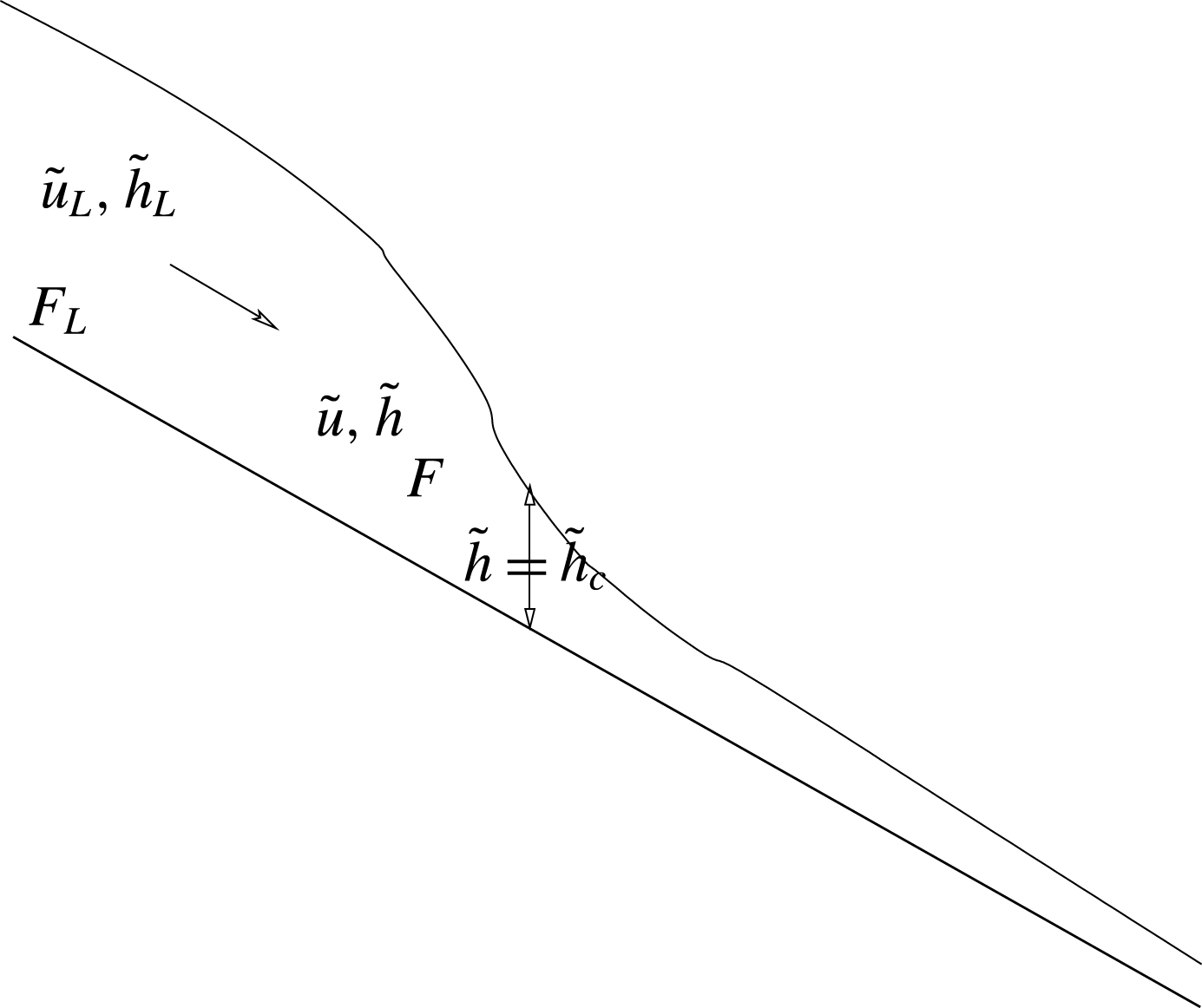
For smooth transition from sub- to supercriticality down a slope we need a situation like that depicted in figure 19.
Smooth flow on a constant slope from sub- to supercritical conditions.

This flow is described by (2.39). Note that the right-hand side of (2.39)
 ${>}0$
for all
 $\tilde{x}$
; therefore the left-hand side
 ${>}0$
as well.
If we differentiate the left-hand side of (2.39) with respect to
 $x$
we get
 $$\begin{eqnarray}\displaystyle \tilde{h}\tilde{h}_{\tilde{x}}-F_{L}^{2}\frac{\tilde{h}_{\tilde{x}}}{\tilde{h}^{2}} & = & \displaystyle \tilde{h}_{\tilde{x}}\left\{\tilde{h}-\frac{F_{L}^{2}}{\tilde{h}^{2}}\right\}\nonumber\\ \displaystyle & = & \displaystyle \tilde{h}\tilde{h}_{\tilde{x}}\left\{1-\frac{F_{L}^{2}}{\tilde{h}^{3}}\right\}.\end{eqnarray}$$
However, for the flow in figure 19,
 $\tilde{h}_{\tilde{x}}<0$
. Therefore, we must have
 $$\begin{eqnarray}\displaystyle 1-\frac{F_{L}^{2}}{\tilde{h}^{3}}<0. & & \displaystyle\end{eqnarray}$$
Now,
 $$\begin{eqnarray}\displaystyle & \displaystyle F^{2}=\frac{\hat{u} ^{2}}{g{\hat{h}}}=\frac{\hat{u} _{L}^{2}}{g{\hat{h}}_{L}}\frac{\tilde{u} ^{2}}{\tilde{h}}=F_{L}^{2}\frac{1}{\tilde{h}^{3}} & \displaystyle\end{eqnarray}$$
 $$\begin{eqnarray}\displaystyle & \displaystyle \Rightarrow \left\{1-\frac{F_{L}^{2}}{\tilde{h}^{3}}\right\}=\left\{1-F^{2}\right\}. & \displaystyle\end{eqnarray}$$
Therefore, if flow is subcritical the flow cannot exist. Therefore, the flow in figure 19 cannot exist. The authors could not find an example in the literature of this analysis being presented, hence its inclusion here.