Introduction
In recent years, with the continuous development of wireless network technology, 5G and the future 6G technology have become the focus of global attention [Reference Wong, Hsu, Lee and Li1–Reference Al Ka’bi3]. The introduction of 5G technology improves data transmission speed and low-latency performance, and supports ultra-reliable and low-latency communications, massive machine-type communications, and expanded mobile broadband [Reference Li, Yu, Diao and Liu4]. Additionally, Wi-Fi 6E and Wi-Fi 7 expand the usage of 2.4, 5, and 6 GHz, and the communication network will be less congested with higher frequency bands [Reference Ding, Rao and Feng5, Reference Li, Zhang and Li6]. The Sub-6 GHz band can take into account both long-distance transmission and reliable network coverage, so many mobile communication devices choose to optimize antenna performance in this frequency band to ensure communication stability and efficiency [Reference Neamah, Al Sabbagh and Al-Rizzo7]. In response to the development of 5G and 6G technologies, multiple-input multiple-output (MIMO) technology has become one of the indispensable technologies in modern wireless communication systems. MIMO antenna technology can mainly improve spectrum efficiency to meet the growing demand for data transmission [Reference Wong, Hong and Li8, Reference Hassan, Saeed, Ali, Cheema and Bermak9]. MIMO technology can simultaneously transmit multiple data channels within the same bandwidth through the layout of multiple antenna units, increasing communication capacity and reducing interference [Reference Abdullah, Kiani, Shoaib, Ali, Elmannai, Algarni and Farooq10, Reference Gu, Li and Li11]. To realize efficient MIMO systems within a limited device size, many studies use innovative antenna designs. For example, parasitic structures are used to reduce mutual coupling effects [Reference Qian, Chen, Liu, Zhou, Wang and Hou12, Reference Mishra, Yadav, Pandey, Chaithra, SethuMadhav, Satheesha and Yadav13], and electromagnetic band gap structures are used to improve antenna isolation and radiation efficiency [Reference Dhasarathan, Tran, Kulkarni, Garner and Li14]. To support 6G high-frequency applications, the development of compact, broadband, and low-mutual-coupling MIMO antenna designs is important. For example, the MIMO antenna system can be configured through an annular ring patch antenna [Reference Wong, Kao and Li15] and a dual-polarized array antenna [Reference Wong, Huang and Li16] to improve overall performance.
In order to achieve high-gain, high-efficiency antennas, many studies have used antenna substrates with low dielectric tangent loss characteristics. This type of substrate helps improve the efficiency and performance of the system. In [Reference Varheenmaa, Ylä-Oijala, Lehtovuori and Viikari17], an RO4350B substrate is configured with open and closed slots to achieve antenna efficiencies of 57.6–84.9%. In [Reference Chen, Liu, Yuan and Wong18], an inverted F antenna structure is used, and the size is reduced through ceramic substrate loading and path folding technology. The extended path forms a ring mode and parasitic branches to achieve dual-band coexistence and achieve good antenna gain. In [Reference Sufyan, Shah, Khan, Shah, Ullah, Siddiqui, Islam and Yoo19], the antenna uses a single-feed structure with a RO4003C substrate and dual-band operation through two F-slot apertures and a slotted ground plane, achieving high isolation and high efficiency without additional decoupling techniques. Although these materials have good dielectric properties, they are too expensive to be mass-produced.
Compared to expensive materials, many studies also use FR-4 substrates to design antennas to achieve the goals of high gain, high efficiency, and low cost. In [Reference Kulkarni, Wang, Zheng, Lin and Chen20], an improved inverted L antenna structure was proposed to enable coverage of 2400–2485 and 5150–7125 MHz with maximum gains of 2.4 and 4.6 dBi, respectively. In [Reference Tang, Chen, Yu, Chen, Che and Xue21], a compact multiband dual antenna system is proposed for Wi-Fi 6E applications. The system incorporates a decoupling inductor between the open ends of the two antennas to achieve low-band decoupling, thus producing a gain effect of 4.27 dBi. In [Reference Chung, Hsu, Lee and Lin22], a multiband antenna suitable for the LTE and 5G NR bands is proposed. This antenna achieved a gain of 4.4 dBi using only a monopole antenna.
In order to achieve multiband operation on a substrate of limited size, many research papers have adopted the integrated design of passive components to improve spectral efficiency and optimize antenna performance. In [Reference Wang and Wu23], a matching circuit was proposed that used distributed capacitors and inductors to adjust the impedance matching and the frequency response. The common and differential modes are adjusted through the shorting pin to achieve good impedance matching within the same frequency range. In [Reference Yan, Zhang, Li, Lin, Guo, Liao and Li24], a balanced multimode loop antenna is proposed that is suitable for the Wi-Fi 6/6E band of a tablet computer with an all-metal case. The antenna improves broadband performance through a segmented ring structure and adjusts effective magnetic permeability through distributed capacitance. This method is used to extend the electric fields of different modes, thereby achieving frequency compression. In [Reference Fang, Liu, Jia, Liang and Zhang25], a reconfigurable low specific absorption rate (SAR) MIMO antenna was proposed and applied to 4G/5G full-screen metal frame smartphones. By deploying the LTE antenna within a narrow ground gap of 2 mm and reconfiguring it with an RF switch, coverage of 698–960 and 1710–2690 MHz is achieved. In [Reference Jabire, Alkhoori, Ghaffar, Faouri, Dahir and Hussein26], a coplanar waveguide-fed MIMO antenna is designed with frequency and reconfigurability characteristics for Wireless LAN (WLAN) and X-band. The system uses PIN diodes for reconfigurable frequency band design to achieve multi-band operation. In [Reference Tang, Sui, Wang, Li, Li and Zhu27], a MIMO antenna design method based on dual-frequency self-decoupling is proposed to generate two frequency bands of 3300–3800 and 4800–5000 MHz, with bandwidths of 500 and 200 MHz, respectively. In [Reference Wong, Chen and Li28], a MIMO antenna was designed consisting of four short-circuit patches of dual band, in which two short-circuit patches of different sizes were used. Each antenna generates 2400 and 5800 MHz frequency bands with bandwidths of 84 and 150 MHz, respectively, and is used for dual-band WLAN applications. In [Reference Munusami and Venkatesan29], a dual-band antenna is proposed, covering 2220–2420 and 5142–5706 MHz, with bandwidths of 200 and 564 MHz, respectively. The antenna achieves good isolation and frequency band coverage by adding an innovative hybrid decoupling structure between the bottom and top of the radiating element. The above studies show that antenna designs that incorporate passive components require higher costs and design complexity to implement multiband antenna systems.
This study presents a low-cost multi-resonant MIMO antenna system designed for integration into laptops and smartphones. Built on a low-cost FR4 substrate, the antenna employs asymmetrical microstrip structures with branch, L-shaped, and S-shaped elements to enhance multi-band operation without passive components. It supports LTE, Sub-6 GHz, and Wi-Fi 6E/7 bands with excellent impedance matching. Structural effects on S-parameters and surface currents are analyzed to improve gain, isolation, and efficiency. Measurements confirm a maximum gain of 9.32 dBi, and SAR/PD simulations validate compliance with international exposure limits.
Antenna design
Single antenna design
Figure 1 shows the proposed LM (low-cost, multi-resonant) antenna structure design, and the detailed dimensions are shown in Table 1. The antenna length and width are 60 and 10 mm, respectively, and a 0.8 mm thick FR4 substrate (dielectric constant 4.4) is used. The green area is the FR4 substrate, and the orange and black areas are copper. The antenna is designed with three branches extending from the ground and one feeding branch to produce multiple resonances, thereby realizing multiple frequency bands at the same time. LM antenna design: To achieve good radiation and impedance matching, the design is carried out according to (1) [Reference Kaushik, Dhanoa and Khandelwal30].
 \begin{align}
w_f & = \frac{2h}{\pi}\left\{[B - 1 - ln(2B - 1)] + \frac{\varepsilon_r - 1}{2\varepsilon_r}\right.\cr
& \qquad \left.\times \left[ln(B - 1) + 0.39 - \frac{0.61}{\varepsilon_r}\right]\right\},
\quad B = \frac{377\pi}{100\sqrt{\varepsilon_r}}
\end{align}
Structure of the LM antenna design.

Figure 1 Long description
Two separate schematic parts are shown on a rectangular substrate outline. The upper part contains the main antenna layout with a long horizontal rectangular trace running across most of the width, with multiple stepped sections and several parallel rectangular stubs grouped on the right side. Near the middle of this upper layout, a narrow vertical connection drops down from the main trace to a short horizontal segment and a small circular marker labeled A is placed at the end of that segment. Two small circular markers labeled B and C are placed close together below the same central area, aligned under the feed region. Along the upper layout, many dimension callouts are drawn with thin dimension lines and arrowheads, labeled W1, W2, W3, W4, W5, W6, W7, W8, W9, W10, W11, W12, W13, W14, W15, W16 and W17 and length callouts labeled L1, L2, L3, L4, L5, L6, L7, L8, L9, L10, L11, L12, L13, L14, L15, L16 and L17. These labels are placed beside the corresponding widths and lengths of the rectangular trace segments and stubs, including several L labels positioned beside the right side stub group and several W labels placed above or within the long horizontal sections. The lower part shows a separate simplified trace segment on another substrate rectangle, consisting of a vertical rectangular trace rising from a circular marker labeled D, then turning into a horizontal rectangular trace to the right, with dimension labels W16 and W17 placed along the horizontal section and L17 placed beside the vertical section. No numeric dimension values or measurement units are printed next to the W and L labels in the figure.
LM antenna detailed dimensions

Table 1 Long description
LM antenna geometric parameters are listed as paired width values W1 through W17 and length values L1 through L17, all measured in millimeters. The largest width is W1 at 60 mm, followed by W2 at 33 mm and W9 at 22 mm, while many widths are small, including W5, W8, and W15 at 2 mm or less. The longest length is L1 at 10 mm, with the next largest lengths L9 at 8.5 mm and L7 at 5 mm. Most lengths are under 4 mm, including several very small features such as L13, L15, and L16 at 1 mm or less. Overall, the design combines one dominant width and one dominant length with many fine-detail dimensions clustered in the low single-digit millimeter range. Values are presented as nominal dimensions without stated tolerances or manufacturing notes, so allowable variation is not indicated.
where  ${W_{f{ }}}$ is the microstrip line feed width,
 ${\varepsilon _r}$ is the substrate dielectric constant, and
 $h$ is the substrate thickness. To account for grounding and substrate boundary effects,
 ${W_{f{ }}}$ is the effective dielectric constant
 ${\varepsilon _{eff}}$, as shown in (2).
 \begin{equation}{\varepsilon _e}ff = \frac{{{\varepsilon _r} + 1}}{2} + \frac{{{\varepsilon _r} - 1}}{2}{\left( {\sqrt {1 + \frac{{12h}}{{{W_f}}}} } \right)^{ - 1}}\end{equation}
Finally, the microstrip line length  ${W_{f{ }}}$ is designed using
 ${\varepsilon _{eff}}$ as shown in (3). Where
 $c$ represents the speed of light and
 ${f_d}$ is the target operating frequency.
 \begin{equation}{L_f} = c \times {\left( {4{f_d}{{\sqrt \varepsilon }_{eff}}} \right)^{ - 1}}\end{equation}
The front and back surfaces are designed based on the calculated characteristic impedance to ensure that the antenna achieves the best impedance matching in the operating frequency band [Reference Kaupp31]. The characteristic impedance can be calculated by (4).
 \begin{equation}{Z_0} = \frac{{87}}{{\sqrt {{\epsilon _r}} + 1.41}}\ln \left[ {\frac{{5.98h}}{{0.8w + t}}} \right]\end{equation}
Based on the parameter analysis results, 1 mm is selected as the feeding branch’s width to optimize the antenna’s impedance matching. where  $h$ is the substrate thickness,
 $w$ is the conductor width,
 $t$ is the conductor thickness (
 $t$ represents the antenna conductor thickness of 0.035 mm), and
 ${ \in _r}$ is the relative dielectric constant of the substrate material.
Antenna evolution
Figure 2 shows the results of the analysis of the evolution of the antenna structure. In Step 1, two branches, A-B and C-D, were designed. This procedure produces a resonance point close to −5.8 dB at 970 MHz at low frequencies (<1 GHz), which covers 1700–2240 MHz at a criterion of −6 dB. A lot of literature uses −6 dB as the bandwidth standard in the application bands of notebook computers and smartphones [Reference Kulkarni, Wang, Zheng, Lin and Chen20, Reference Hu and Li32]. In Step 2, branches at points D-F and F-E are designed to increase the low-frequency resonance depth so that the antenna can generate 950–960 MHz at a −6 dB standard. In Step 3, the D-E branch is designed to expand the low-frequency and high-frequency (>1 GHz) bandwidth. The simulation results show that the low-frequency bandwidth (930–1030 MHz) increases from 10 to 60 MHz, while the high-frequency bandwidth (1810–2310 MHz) increases from 470 to 500 MHz. Step 4 adds an L-shaped path (G-H point) to optimize the high-frequency resonance further so that the antenna can cover 4300–4360 and 5390–9000 MHz. Finally, in step 5, the antenna coupling produces 5370–8980 MHz. An L-shaped ground branch is designed on the back of the antenna to generate more resonance and enhance impedance matching [Reference Chung, Hsieh, Hsu and Lin33, Reference Chung, Huang, Hsu and Lin34]. The proposed antenna covers the following frequency bands under the −10 dB standard: 930–1020, 2020–2260, 2360–2410, 3510–3670, 5470–6240, and 6540–7420 MHz, with an overall frequency band coverage of approximately 46.7% compared to the standard antenna at −6 dB.
Evolution of the LM antenna and variations of the S-parameters. (a) Evolution steps. (b) S-parameters.

Figure 2 Long description
The image consists of two parts. The first part shows the evolution steps of the LM antenna. In Step 1, two branches labeled A-B and C-D are designed, producing a resonance point close to minus 5.8 decibels at 970 megahertz. Step 2 introduces branches at points D-F and F-E to increase low-frequency resonance depth, generating 950-960 megahertz at a minus 6 decibels standard. Step 3 designs the D-E branch to expand bandwidth, increasing low-frequency bandwidth from 930-1030 megahertz and high-frequency bandwidth from 1810-2310 megahertz. Step 4 adds an L-shaped path at G-H to optimize high-frequency resonance, covering 4300-4360 and 5390-9000 megahertz. Step 5 involves antenna coupling, producing 5370-8980 megahertz, with an L-shaped ground branch at the back to enhance impedance matching. The second part contains two graphs showing S-parameter variations. The left graph plots S-parameters in decibels against frequency in gigahertz, with lines representing Steps 1, 2 and 3 and a dashed line at minus 6 decibels. The right graph shows S-parameters for Steps 4 and 5, also against frequency, with a similar dashed line at minus 6 decibels. Both graphs illustrate the changes in resonance and bandwidth across different steps.
This study also analyzes the length of the branches in Steps 1 and 5, as shown in Fig. 3. In Step 1, the S parameter changes of L1 when the length is 10, 19.5, and 25 mm are analyzed. From S11, the bandwidth effect is best when L1 = 19.5 mm. The antenna can have multiple resonance points in the 970 MHz and 1700–2240 MHz frequency bands. In Step 5, the S parameters are analyzed when the L2 length is 0, 6, and 18 mm. When L2 = 6 mm, S11 can cover 920–1040 and 5370–9000 MHz, showing the best bandwidth effect. Finally, based on the above analysis, the optimal size results of the LM antenna are defined.
Results of the length analysis of the LM antenna branches. (a) Results of the L1 analysis. (b) Results of the L2 analysis.

Figure 3 Long description
The image A showing three stacked rectangular layouts labeled L1 equals 25 millimeter, L1 equals 19.5 millimeter and L1 equals 10 millimeter. Each layout contains a long horizontal bar and a shorter L shaped trace inside the rectangle. Small axis markers near the layouts show X, Y and Z. A line graph is shown to the right. The x-axis is labeled Frequency (Gigahertz), with tick labels from 1 to 9 in increments of 1. The y-axis is labeled S parameter (decibel), ranging from 0 to minus 35 in increments of 5. A dashed horizontal reference line is labeled minus 6 decibel. The legend lists Step 1, Step 2 and Step 3. The Step 1 curve has a dip near 2 Gigahertz to about minus 10 decibel and another dip near 6 Gigahertz to about minus 12 decibel. The Step 2 curve has a deep dip near 2 Gigahertz to about minus 25 decibel and then rises toward about minus 5 to minus 10 decibel by 9 Gigahertz. The Step 3 curve stays near 0 to about minus 8 decibel with a shallow dip near 2 Gigahertz. The image B showing three stacked rectangular layouts labeled L2 equals 18 millimeter, L2 equals 6 millimeter and L2 equals 0 millimeter. Each layout contains a long horizontal bar and a shorter vertical bar connected near one end. Small axis markers near the layouts show X, Y and Z. A line graph is shown to the right. The x-axis is labeled Frequency (Gigahertz), with tick labels from 1 to 9 in increments of 1. The y-axis is labeled S parameter (decibel), ranging from 0 to minus 35 in increments of 5. A dashed horizontal reference line is labeled minus 6 decibel. The legend lists Step 1, Step 2 and Step 3. The Step 1 curve shows dips near 2 Gigahertz to about minus 15 decibel, near 4 Gigahertz to about minus 10 decibel and near 6 Gigahertz to about minus 30 decibel. The Step 2 curve shows dips near 2 Gigahertz to about minus 18 decibel, near 3 Gigahertz to about minus 12 decibel and near 6.5 Gigahertz to about minus 28 decibel. The Step 3 curve shows dips near 2 Gigahertz to about minus 12 decibel and near 5 Gigahertz to about minus 10 decibel, then stays between about minus 5 and minus 10 decibel toward 9 Gigahertz.
Figure 4 shows the simulation results of the surface current of the LM antenna. This study analyzes several important frequency points (0.92, 2, 3.5, 5.8, 6.8, and 7.7 GHz). The analysis results show that the current convergence results are consistent with the analysis of antenna evolution, confirming that this antenna structure has a stable current flow direction. The optimized LM antenna can simultaneously cover 920–1040, 1810–2450, 3480–3780, and 5370–9000 MHz. The 920–1040 MHz frequency band can be used in systems such as RFID and GSM 900. The 1810–2450 MHz band supports 3G/4G LTE mobile communication and Wi-Fi and Bluetooth transmission in the 2.4 GHz band. For next-generation high-speed communications, LM antennas can be used in the 3480–3780 and 5370–9000 MHz bands for 5G NR Sub-6 GHz and Wi-Fi 6E/7.
Results of the LM antenna surface current analysis.

Figure 4 Long description
Six engineering heatmaps of a surface current density quantity on the same elongated structure, shown at six frequencies. Each heatmap includes a frequency label: 920 MHz, 2000 MHz, 3500 MHz, 5850 MHz, 6800 MHz and 7700 MHz. A single color scale at the left indicates surface current density labeled Jsurf [A/m]. The scale values are 100.0000, 93.3333, 86.6667, 80.0000, 73.3333, 66.6667, 60.0000, 53.3333, 46.6667, 40.0000, 33.3333, 26.6667, 20.0000, 13.3333, 6.6667 and 0.0000. At 920 MHz, the strongest surface current density appears as a narrow band near the top trace region and a narrow vertical band at the central junction region. Most other parts of the structure are near the lower end of the scale. At 2000 MHz, a strong band appears along the top trace region and a strong vertical band appears at the central junction region. The parallel trace region on the far right remains near the lower end of the scale. At 3500 MHz, the strongest region is concentrated at the central junction region, forming a vertical band with a short extension into the top trace region. The far-right parallel trace region remains near the lower end of the scale. At 5850 MHz, a strong band runs along the top trace region toward the central junction region and a vertical band is present at the central junction region. The far-right parallel trace region remains near the lower end of the scale. At 6800 MHz, a vertical band at the central junction region is prominent, with a thinner band along the top trace region. The far-right parallel trace region remains near the lower end of the scale. At 7700 MHz, a strong band appears along the top trace region toward the central junction region and a vertical band is present at the central junction region. The far-right parallel trace region remains near the lower end of the scale. Across all six frequencies, the highest surface current density regions repeatedly occur at the central junction region and along the top trace region, while the far-right parallel trace region stays near the lower end of the Jsurf [A/m] scale.
LM MIMO antenna system configuration
Figure 5 shows the configuration of the MIMO antenna system for a laptop computer and a smartphone. The notebook computer is equipped with 10 identical LM antennas on a substrate of 330 × 220 mm2. In this configuration, all antennas have a mirror-image and symmetric relationship. The simulation and measurement results of antennas with mirror-image or symmetrical relationships will be very similar, in the proposed system, only Antenna 1, Antenna 2, and Antenna 10 are needed to deduce all the results. The smartphone has two LM antennas with the same structure configured on a 70 × 120 mm2 substrate. Since Ant 1 and Ant 2 have a symmetrical relationship, it is sufficient to discuss only the simulation and measurement results of Ant 1. To verify the proposed MIMO antenna system, this article actually fabricated a prototype of the LM MIMO antenna system for a laptop and a smartphone, as shown in Fig. 6.
Mirror and symmetry relationships of the LM MIMO antenna system. (a) Laptop. (b) Smartphone.

Figure 5 Long description
The diagram consists of two parts illustrating LM MIMO antenna configurations. On the left, a laptop configuration is shown with a green rectangular substrate labeled ′Laptop size 330 times 220 millimeters squared.′ Ten antennas, labeled Ant 1 to Ant 10, are positioned around the edges. Ant 1 and Ant 2 are at the top, Ant 3 and Ant 4 on the right, Ant 5 and Ant 6 at the bottom and Ant 7 to Ant 10 on the left. Solid arrows indicate mirror relationships, while dashed arrows indicate symmetrical relationships between antennas. On the right, a smartphone configuration is depicted with a smaller green rectangular substrate labeled ′Smartphone size 70 times 120 millimeters squared.′ Two antennas, Ant 1 and Ant 2, are positioned at the top and bottom. The diagram includes a coordinate system in the bottom left corner, labeled X, Y and Z axes. Mirror and symmetrical relationships are indicated by solid and dashed arrows, respectively, at the top right.
Prototype of the LM MIMO antenna system. (a) Laptop. (b) Smartphone.

Figure 6 Long description
The image A shows a laptop-sized substrate measuring 330 by 220 millimeters with ten labeled antennas, Ant 1 through Ant 10, arranged symmetrically around the edges. The antennas are positioned with Ant 1 to Ant 5 on the top and right edges and Ant 6 to Ant 10 on the bottom and left edges. The center of the substrate is marked with the text ′Laptop size 330 by 220 millimeters squared.′ The image B shows a smartphone-sized substrate measuring 70 by 120 millimeters with two labeled antennas, Ant 1 and Ant 2, positioned on the top and bottom edges. The center of this substrate is marked with the text ′Smartphone size 70 by 120 millimeters squared.′ Both substrates are placed on a grid background for scale reference.
Analysis of the MIMO antenna on different devices
S-parameter
Figure 7 shows the measurement setup for different devices. Figure 8 shows the simulation and measurement results of the reflection coefficient on different devices. The S-parameter results show that both systems can cover 920–1030, 1930–2450, 3440–3750, and 5390–9000 MHz. The detailed simulated and measured S parameters are shown in Table 2. The comparison in the table shows that the simulation and measurement results show similar trends, demonstrating good stability. When evaluating the S parameters of mobile devices.
Measurement setup for different devices. (a) Laptop. (b) Smartphone.

Simulated and measured S-parameter results of the LM MIMO antenna system on different devices. (a) Laptop Ant 1. (b) Laptop Ant 2. (c) Laptop Ant 10. (d) Smartphone Ant 1.

Figure 8 Long description
The image consists of two parts comparing LM MIMO antenna systems on different devices. On the left, labeled as Ant 1 through Ant 10, is a laptop-sized setup measuring 330 by 220 millimeters squared. Each antenna is positioned around the perimeter of the rectangular board, with Ant 1, Ant 2, Ant 3 and Ant 4 along the top edge, Ant 5, Ant 6, Ant 7 and Ant 8 along the bottom edge and Ant 9 and Ant 10 on the left edge. The right part shows a smartphone-sized setup measuring 70 by 120 millimeters squared, with Ant 1 and Ant 2 positioned along the top edge. Both setups are placed on a grid background, providing a clear view of the antenna arrangements and device sizes.
Comparison of simulation and measurement of S-parameters of LM MIMO antenna systems with different devices

Table 2 Long description
S-parameter operating frequency ranges in megahertz are listed for simulated versus measured results for three laptop antennas (Ant 1, Ant 2, Ant 10) and one smartphone antenna (Ant 1). For the laptop, simulations cover about 920 to 1030, 1930 to 2450, 3430 to 3750, and 5390 to 9000 for Ant 1, with similar bands for Ant 2 and Ant 10. Measured laptop bands shift lower overall, for example Ant 1 changes to about 910 to 1030, 1730 to 2450, 3250 to 3590, and 5160 to 8270, and Ant 2 and Ant 10 show comparable downward shifts. For the smartphone, simulation spans about 950 to 1070, 1950 to 2420, 3460 to 3730, and 5400 to 7580, while measurement shifts to about 940 to 1040, 1800 to 2440, 3410 to 3870, and 5200 to 8180. Across devices, the lowest band stays close between simulation and measurement, mid bands tend to start at lower frequencies in measurement, and the highest band often becomes narrower or moves downward, especially for the laptop. Differences likely reflect device integration and measurement conditions, so exact band edges should be treated as approximate rather than identical matches.
Figure 9 shows the isolation simulation and measurement results of different devices. The isolation of the LM MIMO antenna system on the notebook computer is kept below −10 dB, and the lowest is close to −68 dB. At the same time, the isolation trends of smartphones and laptops are similar. However, the isolation of both devices is worse below 1.5 GHz than at higher frequencies. As shown in (2) and (3) [Reference Varheenmaa, Ylä-Oijala, Lehtovuori and Viikari17], the main reason for this phenomenon is that the long wavelength of low-frequency signals will cause mutual interference between antennas due to the coupling effect of electric and magnetic fields. Since smartphones are much smaller than laptops, the antennas are closer together, resulting in reduced isolation in the low-frequency band. However, the proposed MIMO antenna system can still maintain good isolation performance on different devices and is not easily affected by the number of antennas or device size.
Simulated and measured S-parameter results of the LM MIMO antenna system on different devices. (a) Laptop Ant 1. (b) Laptop Ant 2. (c) Laptop Ant 10. (d) Smartphone Ant 1.

Figure 9 Long description
Graph A shows the S21 parameter for a laptop. The vertical axis is S-Parameter in decibels from 0 to minus 90 and the horizontal axis is Frequency in gigahertz from 1 to 9. Key dips occur around 2.5 GHz and 5.5 GHz, with simulation and measurement closely aligning, especially near 3 GHz. Graph B displays the S91 parameter for a laptop. The axes are the same as Graph A. Notable dips are at 3 GHz and 6 GHz, with the measured curve generally lower than the simulated one. Graph C presents the S101 parameter for a laptop. The axes remain consistent. Dips are observed around 2 GHz and 5 GHz, with the simulation and measurement diverging more significantly at lower frequencies. Graph D illustrates the S21 parameter for a smartphone. The axes are identical to previous graphs. Major dips occur at 2.5 GHz and 5.5 GHz, with the measured trace higher than the simulated one. Across all graphs, simulated traces are dashed and measured traces are solid. The laptop graphs show broader bandwidths below minus 10 decibels compared to the smartphone, with the deepest notches in Graph B. The comparative analysis highlights the differences in antenna performance between devices and parameter types.
In (5),  $\lambda $ is the wavelength,
 ${d_h}$ is the distance between the two antennas, and
 ${G_{Tx}}\left( \varphi \right)$ and
 ${G_{Rx}}\left( \varphi \right)$ are the antenna pattern parameters defined in the far field. In (6), it is mainly used to calculate vertical isolation. If
 $d \lt 0.2\lambda $,
 ${I_v}\left[ {dB} \right]$ is negative, indicating that the received power is greater than the transmitted power [Reference Feng, Gao, Rao, Shi, Shen, Zhang and Meng35].
 \begin{equation}{I_H}\left| {dB} \right| = 22 + 20lg\frac{{dh}}{\lambda } - \left[ {{G_{Tx}}\left( \varphi \right) + {G_{Rx}}\left( \varphi \right)} \right]\end{equation}
 \begin{equation}{I_v}\left| {dB} \right| = 28 + 40lg\frac{1}{\lambda }\end{equation}
Antenna performance analysis
This paper measures the antenna performance in the same coordinate system as the simulation, as shown in Fig. 10. Figures 11 and 12 show the gain and efficiency results for different devices. Different frequency points (920, 2000, 6800, and 7700 MHz) are analyzed and discussed, respectively. The proposed MIMO system can achieve a gain effect close to 9.32 dBi within the frequency band. This result shows that the system has stronger anti-interference performance and signal strength. In terms of efficiency, the maximum efficiency in low frequency and high frequency can reach 72% and 84%, respectively. The above measurement results are consistent with the trends presented by the simulation results.
Measurement setup of different devices in a darkroom. (a) Smartphone. (b) Laptop.

Simulated and measured gain results of the LM MIMO antenna system on different devices. (a) Laptop Ant 1. (b) Laptop Ant 2. (c) Laptop Ant 10. (d) Smartphone Ant 1.

Figure 11 Long description
The multi-line graphs compare measured and simulated gain results for different antennas on laptops and a smartphone. Each subplot represents a different antenna: (a) Laptop Ant. 1, (b) Laptop Ant. 2, (c) Laptop Ant. 10 and (d) Smartphone Ant. 1. The horizontal axis is labeled Frequency in GHz, ranging from 0 to 9. The vertical axis is labeled Gain in dBi, ranging from negative 15 to 20. Solid lines represent measured gain, while dashed lines represent simulated gain. In subplot (a), Laptop Ant. 1 shows a general increase in gain with peaks around 3 GHz and 7 GHz. The simulated gain slightly overestimates the measured gain at higher frequencies. In subplot (b), Laptop Ant. 2 displays a similar trend with peaks near 3 GHz and 7 GHz, with the simulation closely matching the measured gain. In subplot (c), Laptop Ant. 10 shows fluctuations with notable peaks around 3 GHz and 6 GHz. The simulated gain generally follows the measured trend but diverges slightly at higher frequencies. In subplot (d), Smartphone Ant. 1 exhibits peaks around 2 GHz and 6 GHz, with the simulation underestimating the measured gain at lower frequencies. These graphs highlight the differences in gain performance between measured and simulated results across various frequencies for each antenna.
Simulated and measured efficiency results of the LM MIMO antenna system on different devices. (a) Laptop Ant 1. (b) Laptop Ant 2. (c) Laptop Ant 10. (d) Smartphone Ant 1.

Figure 12 Long description
The graphs compare simulated and measured efficiency of antennas on different devices. Each graph has the horizontal axis labeled ′Frequency (GHz)′ and the vertical axis labeled ′Efficiency (%)′. The graphs are titled ′Laptop Ant. 1′, ′Laptop Ant. 2′, ′Laptop Ant. 10′ and ′Smartphone Ant. 1′. The simulated data is shown with a dashed line, while the measured data is shown with a solid line. For ′Laptop Ant. 1′, efficiency fluctuates between 40 percent and 80 percent across frequencies, with peaks around 3 GHz and 6 GHz. The simulated and measured lines generally align, with minor deviations. In ′Laptop Ant. 2′, efficiency ranges from 30 percent to 90 percent, peaking near 2 GHz and 7 GHz. The simulated line is consistently higher than the measured line, especially between 4 GHz and 6 GHz. For ′Laptop Ant. 10′, efficiency varies from 40 percent to 85 percent, with notable peaks at 3 GHz and 7 GHz. The simulated and measured lines show similar trends, with slight divergence around 5 GHz. In ′Smartphone Ant. 1′, efficiency ranges from 30 percent to 80 percent, with peaks at 2 GHz and 6 GHz. The simulated line is higher than the measured line, particularly between 4 GHz and 5 GHz. Overall, the graphs illustrate how efficiency varies across frequencies and devices, highlighting where simulated and measured results align or differ.
Figures 13 and 14 show the 2D radiation direction analysis results of different MIMO systems; from left to right, they are the XY, XZ, and YZ planes, respectively. Figures 15 and 16 show the 3D radiation direction simulation results of different devices. The proposed MIMO antenna system is simulated and measured at frequencies of 920, 2000, 3500, 5850, 6800, and 7700 MHz. The figure shows that the antennas all show an omnidirectional trend despite being configured in different devices. The results confirm that the LM antenna can provide an extensive transmission and reception range when configured with different electronic devices.
Simulated and measured 2D radiation results of the LM MIMO antenna system on laptop: (a) 920 MHz, (b) 2000 MHz, (c) 3500 MHz, (d) 5850 MHz, (e) 6800 MHz, and (f) 7700 MHz.

Figure 13 Long description
Polar plots display the 2D radiation patterns of the LM MIMO antenna system at frequencies 920MHz, 2000MHz, 3500MHz, 5850MHz, 6800MHz and 7700MHz. Each frequency is represented across three planes: XY, XZ and YZ. The radial axis represents gain in decibels, ranging from 10 to minus 60. Four traces are shown: Measured Phi, Simulated Phi, Measured Theta and Simulated Theta. The plots generally exhibit near-circular patterns with minor ripples. Notable features include notches near minus 50 and minus 60 decibels and bulges near 0 and 10 decibels. The measured and simulated patterns closely match, with some variations in specific planes and frequencies. The deepest nulls and strongest lobes vary, with the most significant deviations observed at higher frequencies. These plots illustrate the antenna′s omnidirectional radiation characteristics under different configurations.
Simulated and measured 2D radiation results of the LM MIMO antenna system on smartphone: (a) 920 MHz, (b) 2000 MHz, (c) 3500 MHz, (d) 5850 MHz, (e) 6800 MHz, and (f) 7700 MHz.

Figure 14 Long description
Simulated and measured 2D radiation results of the LM MIMO antenna system on smartphone: (a) 920 MHz, (b) 2000 MHz, (c) 3500 MHz, (d) 5850 MHz, (e) 6800 MHz and (f) 7700 MHz. Each frequency has three polar plots for XY, XZ and YZ planes. The radial axis represents gain in decibels. The legend includes Measured Phi, Simulated Phi, Measured Theta and Simulated Theta. For each frequency, the XY and YZ planes generally show near-circular patterns with slight dips around 180 degrees. The XZ plane becomes more multi-lobed as frequency increases, indicating more complex radiation patterns. Agreement between measured and simulated data is generally good, with some deviations in the XZ plane at higher frequencies. Key quantitative features include approximate peak levels and null depths, with notable angular directions for maxima and minima. The plots provide insights into the antenna′s omnidirectional trend and performance across different planes and frequencies.
Simulated 3D radiation results of the LM MIMO antenna system on laptop.

Figure 15 Long description
Six 3D spherical radiation patterns labeled (a) through (f) display simulated gain values for the LM MIMO antenna system configured on a laptop. Each pattern is plotted in a spherical coordinate system where the azimuth angle spans 0 to 360 degrees and the elevation angle spans 0 to 180 degrees. The radial dimension of each sphere directly represents gain in decibels. The shared color scale ranges from plus 10 decibels at the upper end to minus 30 decibels at the lower end. Directional reference markers are placed at azimuth positions of 0, 90, 180 and 270 degrees on each plot. In panel (a), the radiation pattern appears largely uniform across most azimuth and elevation angles, with gain values concentrated near the upper range of the scale, suggesting a broadly distributed lobe structure with minimal deep nulls. In panel (b), the pattern retains broad coverage but shows slight variation in gain across elevation angles, with the upper hemisphere showing higher gain values compared to the lower hemisphere. In panel (c), the distribution is similar to panel (b), with high gain values across a wide azimuth range and a gradual reduction toward the lower elevation angles. In panel (d), the pattern shows a more irregular shape, with a visible reduction in gain in certain azimuth sectors and the lower hemisphere displays notably lower gain values approaching the minus 25 to minus 30 decibel range. In panel (e), the pattern exhibits a pronounced asymmetry, with one sector showing concentrated high gain near plus 5 to plus 10 decibels and opposing sectors showing gain values near minus 20 decibels. In panel (f), the radiation pattern shows two distinct lobes separated by a visible null region, with peak gain values near plus 5 to plus 10 decibels and minimum values near minus 25 decibels in the null zones. Across all six panels, the peak gain values fall within the plus 5 to plus 10 decibel range, while the deepest nulls approach minus 25 to minus 30 decibels.
Simulated 3D radiation results of the LM MIMO antenna system on smartphone.

Figure 16 Long description
Six simulated 3D far-field radiation patterns are arranged in two rows of three, labeled (a) through (f), for an LM MIMO antenna system configured on a smartphone. Each plot displays total realized gain in decibels using a shared color scale ranging from minus 30 decibels at the lower end to 10 decibels at the upper end. The angular axes represent azimuth and elevation angles in degrees, spanning the full spherical far-field space around the antenna structure. The three-dimensional surface shape in each panel represents the magnitude of the radiated gain in all directions. Panel (a) shows a near-hemispherical radiation shape with the primary lobe oriented upward along the vertical axis. The pattern is relatively broad with a visible reduction in gain toward the lower hemisphere. Panel (b) displays a more elongated pattern with a dominant lobe extending along the upper vertical direction. A visible constriction or narrowing is present near the equatorial region, suggesting a more directive response compared to panel (a). Panel (c) presents a broadly distributed pattern with moderate gain across the upper hemisphere. The shape appears rounded with a slight asymmetry toward one lateral side. Panel (d) shows a pattern with a pronounced lobe displaced laterally, with deeper nulls visible toward the lower hemisphere. The gain distribution is less symmetric compared to panels (a) through (c). Panel (e) displays a pattern with a dominant lobe shifted toward one side, with the main radiation concentrated in a localized angular region. Deeper null regions are visible on the opposite side. Panel (f) presents a pattern with the most asymmetric shape among all six panels. A large lobe extends prominently to one lateral side, with significant gain reduction visible across the opposing hemisphere. Across all six panels, the patterns retain broad angular coverage in the upper hemisphere while showing varying degrees of asymmetry, lobe direction and null depth in the lower hemisphere. The color scale markings visible on the left side of the composite figure indicate values at 10, 5, 0, minus 5, minus 10, minus 15, minus 20, minus 25 and minus 30 decibels.
Figure 17 shows the simulation and measurement results of the envelope correlation coefficient (ECC) on different devices. ECC is used to evaluate whether a MIMO antenna can effectively provide multiple independent transmission channels. 0.5 is a common evaluation standard for electronic devices [Reference Chung, Hsu, Lee and Lin22]. The simulation and measurement results show that the overall ECC of the antenna in both systems is less than 0.5, indicating that the antennas in different systems have good independence. However, the ECC value is relatively high when the frequency is below 1.5 GHz, which is directly related to reducing low-frequency isolation, as shown in (7) [Reference Chung, Hsu, Lee and Lin22]. When the isolation between antennas is poor, the absolute values of S12 and S21 will be larger, resulting in an increase in the numerator and an increase in the ECC value. The smaller ground plane of smartphones shortens the antenna spacing, further causing the antennas to affect each other, resulting in the ECC being slightly higher at low frequencies than in other frequency bands. Overall, the ECC remains below 0.5, ensuring good channel independence for the MIMO system.
 \begin{equation}{\text{ECC}} = \frac{{{{\left| {{S_{11}}S_{12}^* + {S_{21}}S_{22}^*} \right|}^2}}}{{\left( {1 - {{\left| {{S_{11}}} \right|}^2} - {{\left| {{S_{21}}} \right|}^2}} \right)\left( {1 - {{\left| {{S_{22}}} \right|}^2} - {{\left| {{S_{12}}} \right|}^2}} \right)}}\end{equation}
ECC results of the LM MIMO antenna system. (a) Laptop. (b) Smartphone.

Effect of the human body and SAR analysis
To verify the impact of the human body on the antenna performance of laptops and smartphones in actual holding and talking situations. This paper introduces two human models, hands and face, into the simulation for evaluation, as shown in Fig. 18(a) and (b). The simulations were configured with different human contact scenarios for laptops and smartphones. The short sides of the laptops are covered by both hands, simulating the impact of a user holding the notebook in hand. The smartphone is held close to the face and ear to simulate a phone call.
Simulation configuration of different devices in actual scenarios. (a) Handheld laptop. (b) Answering a smartphone call.

Figure 19(a) and (b) shows the impact of different usage scenarios on the antenna. The simulation results show that the simulation trends of the covered device and the uncovered device are similar, which proves its good stability.
S-parameter simulation results under different usage scenarios. (a) Handheld laptop. (b) Answering a smartphone call.

Figure 19 Long description
Two S-parameter line plots display frequency response from 1 to 9 GHz. The X-axis is labeled Frequency in GHz and the Y-axis is labeled S-parameter in decibels. Panel (a) includes traces for simulated S11, S21, S22 and S10, with specified targets shown as dashed lines. Notable minima occur around 2.5 GHz and 5.5 GHz, with depths reaching below minus 40 decibels. Panel (b) focuses on S11 and S10, showing similar trends with minima at similar frequencies. The plots illustrate how closely the simulated results match the specified targets, highlighting performance across different frequency bands.
Specific absorption rate (SAR) is a basic indicator used to evaluate the absorption of electromagnetic wave energy of the human body by wireless communication equipment. The testing and analysis of SAR values must meet international standards, which is very important for antenna design. The SAR value is calculated by the rate of electromagnetic energy absorbed per unit of mass of human tissue, and its unit is W/kg. The SAR value can be calculated by (8) [Reference Chung, Hsu, Lee and Lin22].
 \begin{equation}SAR = \frac{d}{{dt}}\left( {\frac{{dw}}{{DM}}} \right) = \frac{d}{{dt}}\left( {\frac{{dW}}{{\rho dV}}} \right)\end{equation}
The values of SAR and PD are recorded in Tables 3 and 4. Figure 20 shows the simulated configuration of different devices placed in the human body. Figures 21–24 show the SAR simulation results of different devices on the human body at an input power of 0.1 W. To ensure user safety, global standards cap the average SAR at below 1.6 W/kg for 1 gram of tissue [36], and below 2 W/kg for 10 grams of tissue [Reference Chou, D’Andrea and Peterson37], thus ensuring that the device does not cause radiation hazards to the human body. Above 6000 MHz, the primary exposure limit transitions from SAR to free-space power density (PD), expressed in W/m2. The FCC regulations limit the radiated power to less than 40 and 10 W/m2 per 1 cm2 and 4 cm2 area, respectively [Reference Colombi, Thors and Törnevik38]. Finally, the results of the analysis confirmed that the proposed devices all meet the standard values. The PD value can be calculated by (9) [Reference Chung, Lin and Yang39]:
 \begin{equation}{S_{inc}}\left( {A,d,{\beta _X}} \right) = \frac{1}{A} \int _A {\text{Re}}\left[ {E\left( {d,{\beta _X}} \right) \times {H^*}\left( {d,{\beta _X}} \right)} \right] \cdot \hat n\,ds\end{equation}
Human body SAR simulation configurations for different devices. (a) Laptop placed on the lap. (b) Smartphone placed near the face. (c) Smartphone held in hand.

Simulated SAR and PD results for a laptop on the human lap at different frequencies. (a) SAR. (b) PD.

Figure 21 Long description
The image consists of two sections labeled as (a) and (b). Section (a) displays simulated Specific Absorption Rate (SAR) results for a laptop on the human lap at various frequencies. There are four sub-images, each showing a human silhouette with color-coded SAR values. The frequencies are 920 MHz, 2400 MHz, 3500 MHz and 5850 MHz, with corresponding SAR values of 0.149 W/kg, 0.614 W/kg, 1.02 W/kg and 1.04 W/kg for 1 gram of tissue and 0.0848 W/kg, 0.358 W/kg, 0.239 W/kg and 0.341 W/kg for 10 grams of tissue. Each sub-image includes a color scale indicating the intensity of SAR values. Section (b) presents simulated Power Density (PD) results for the same setup at frequencies of 6800 MHz and 7700 MHz. There are four sub-images, each showing a human silhouette with color-coded PD values. The PD values are 27.3 W m superscript -2 and 8.1 W m superscript -2 for 1 cm superscript 2 and 0.547 W m superscript -2 and 0.162 W m superscript -2 for 4 cm superscript 2. Each sub-image includes a color scale indicating the intensity of PD values. The diagrams visually represent the distribution of SAR and PD across the human body at different frequencies.
Simulated 1 g SAR and 1 cm2 PD results for a smartphone near the face at different frequencies. (a) SAR. (b) PD.

Figure 22 Long description
The image consists of two parts labeled as (a) and (b). Part a shows simulated specific absorption rate (SAR) results for a smartphone near the face at four different frequencies: 920 megahertz, 2000 megahertz, 3500 megahertz and 5850 megahertz, each with a 1 gram average. Each frequency is accompanied by a color scale indicating SAR values in watts per kilogram, with specific values noted, such as 0.0209 for 920 megahertz and 0.189 for 5850 megahertz. Part b displays power density (PD) results at two frequencies: 6800 megahertz and 7700 megahertz, each with a 1 square centimeter average. The color scale for PD is in watts per square meter, with values like 0.0029 for 6800 megahertz and 2.3 for 7700 megahertz. Both parts illustrate the distribution of SAR and PD on a human head model, highlighting areas of higher absorption and density with varying color intensities.
Simulated 10 g SAR and 4 cm2 PD results for a smartphone near the face at different frequencies. (a) SAR. (b) PD.

Figure 23 Long description
The image consists of two sections labeled as (a) and (b), each showing simulated results for a smartphone near the face at different frequencies. Section (a) displays four simulations of Specific Absorption Rate (SAR) at frequencies 920 MHz, 2000 MHz, 3500 MHz and 5850 MHz, all measured in 10 grams. Each simulation includes a color scale indicating SAR values, with the scale ranging from low to high absorption. The SAR distribution is visualized on a human head model, highlighting areas of higher absorption near the ear and cheek. Section (b) presents two simulations of Power Density (PD) at frequencies 6800 MHz and 7700 MHz, measured in 4 square centimeters. Similar to section (a), each simulation includes a color scale indicating PD values, with the scale ranging from low to high density. The PD distribution is visualized on the same head model, showing areas of higher density near the ear and forehead. Both sections illustrate how frequency affects SAR and PD distribution on the head model.
Simulated SAR and PD results for a smartphone in hand at different frequencies. (a) SAR. (b) PD.

Figure 24 Long description
Simulated SAR and PD results for a smartphone in hand at different frequencies. (a) SAR. (b) PD. (a) Avg SAR heatmaps on body silhouettes with a vertical legend labeled Avg SAR in W per kilogram. The legend shows higher values at the top and lower values at the bottom. Each frequency is shown for 1 g and 10 g. 920 megahertz, 1 g: Avg SAR value 0.0104 W per kilogram. 920 megahertz, 10 g: Avg SAR value 0.246 W per kilogram. 2400 megahertz, 1 g: Avg SAR value 0.852 W per kilogram. 2400 megahertz, 10 g: Avg SAR value 0.563 W per kilogram. 3500 megahertz, 1 g: Avg SAR value 0.281 W per kilogram. 3500 megahertz, 10 g: Avg SAR value 0.189 W per kilogram. 5850 megahertz, 1 g: Avg SAR value 0.681 W per kilogram. 5850 megahertz, 10 g: Avg SAR value 0.324 W per kilogram. Across the Avg SAR set, the listed values are higher at 2400 megahertz than at 920 megahertz for both 1 g and 10 g. For 2400 megahertz, 3500 megahertz and 5850 megahertz, the 1 g value is higher than the 10 g value. For 920 megahertz, the 10 g value is higher than the 1 g value. Hotspots appear as limited regions on each silhouette rather than being uniform across the full body shape. (b) PD heatmaps on body silhouettes with a vertical legend labeled PD in W per m superscript 2. The legend shows higher values at the top and lower values at the bottom. Each frequency is shown for 1 centimeter superscript 2 and 4 centimeter superscript 2. 6800 megahertz, 1 centimeter superscript 2: PD value 4.08 W per m superscript 2. 6800 megahertz, 4 centimeter superscript 2: PD value 3.4 W per m superscript 2. 7700 megahertz, 1 centimeter superscript 2: PD value 3.4 W per m superscript 2. 7700 megahertz, 4 centimeter superscript 2: PD value 5.3 W per m superscript 2. Across the PD set, the listed value decreases from 4.08 to 3.4 for 1 centimeter superscript 2 when moving from 6800 megahertz to 7700 megahertz, while the listed value increases from 3.4 to 5.3 for 4 centimeter superscript 2. Hotspots appear as limited regions on each silhouette.
Simulated SAR values of the LM MIMO antenna system on different devices

Table 3 Long description
Simulated specific absorption rate values are listed for a LM MIMO antenna on two device types, reported as 1 g SAR and 10 g SAR in watts per kilogram at 920, 2400, 3500, and 5850 MHz. For the laptop (lap position), 1 g SAR rises from 0.149 at 920 MHz to 0.614 at 2400 MHz, then to 1.02 at 3500 MHz and 1.04 at 5850 MHz; 10 g SAR ranges from 0.0848 to 0.358, 0.239, and 0.341 across those frequencies. For the smartphone at the face, 1 g SAR is lowest at 920 MHz (0.0104) and highest at 2400 MHz (0.852), with 10 g SAR peaking at 2400 MHz (0.563). For the smartphone in the hand, 1 g SAR is low at 920 and 2400 MHz (0.0209 and 0.0132) but peaks at 3500 MHz (0.895); 10 g SAR follows the same pattern, highest at 3500 MHz (0.411). Comparing devices, the laptop shows the overall highest 1 g SAR values at 3500 and 5850 MHz, while the smartphone’s highest exposures depend on use position (face at 2400 MHz, hand at 3500 MHz). Values are simulated and may vary with modeling assumptions, device placement, and user proximity.
Simulated PD values of the LM MIMO antenna system on different devices

Table 4 Long description
Simulated power density values are listed for an LM MIMO antenna system on a laptop and a smartphone, reported at 6800 and 7700 MHz for averaging areas of 1 cm squared and 4 cm squared, in watts per square meter. For the laptop, values drop sharply when moving from 1 cm squared to 4 cm squared: 27.3 to 0.547 at 6800 MHz, and 8.1 to 0.162 at 7700 MHz. For the smartphone at the face position, values remain high at both areas: 18 to 14.4 at 6800 MHz, and 21.2 to 16.3 at 7700 MHz. For the smartphone in the hand position, values are lower than the face position and change modestly with area: 4.08 to 3.4 at 6800 MHz, and 3.4 to 5.3 at 7700 MHz. Comparing devices, the smartphone face readings are much higher than the laptop at 4 cm squared at both frequencies, while the laptop is higher than the smartphone face at 1 cm squared at 6800 MHz but lower at 7700 MHz. Differences reflect both device type and body location, and results are simulated values that may vary with real-world use and positioning.
Where  ${\text{Re}}$ is the real part,
 $A$ is the average area, and
 $d$ is the distance between the antenna and the tissue.
Comparing the performance of different antennas
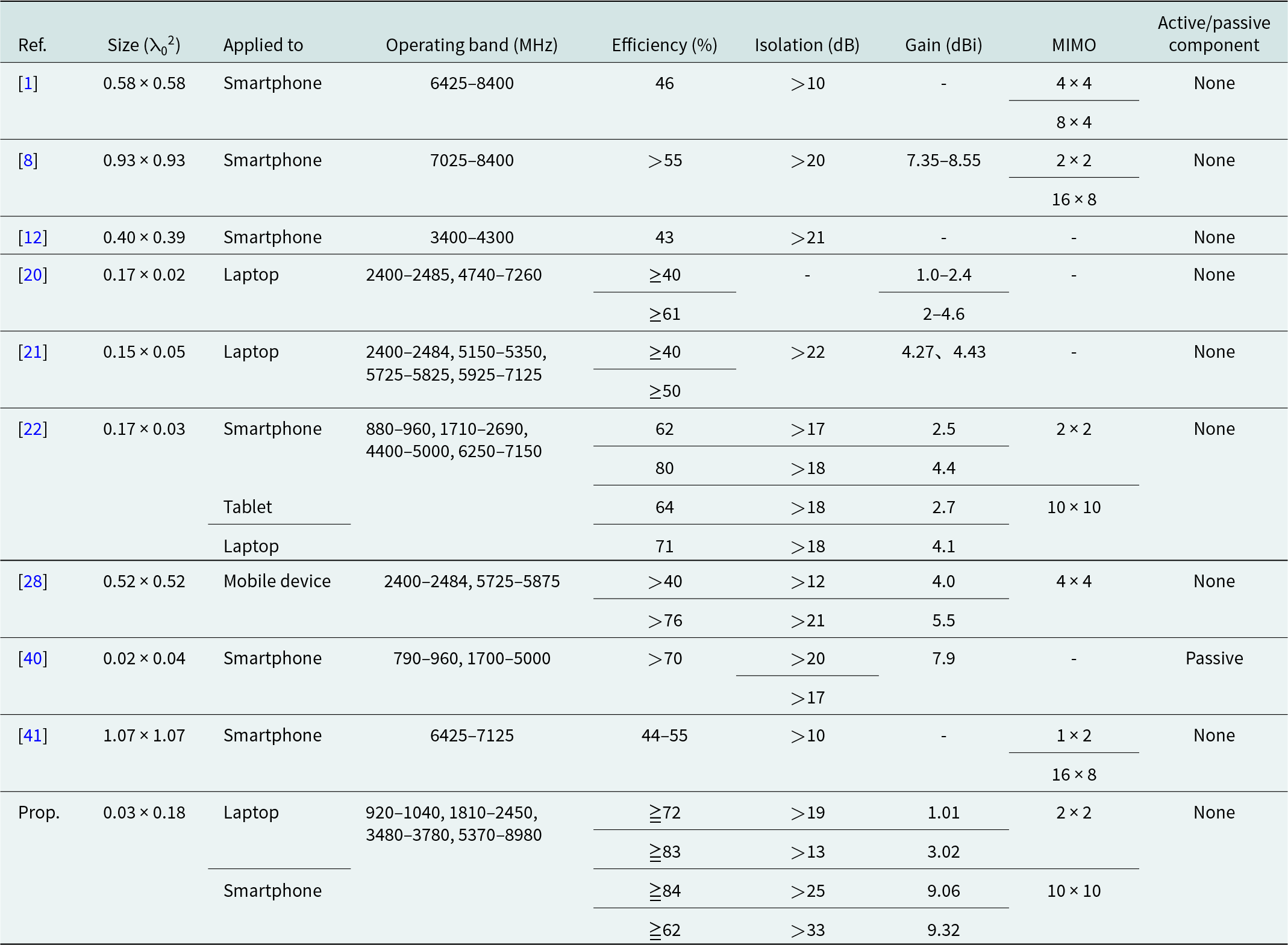
As summarized in Table 5, the proposed LM MIMO antenna system demonstrates clear advantages over recently reported designs for portable electronic devices. While prior works such as [Reference Tang, Chen, Yu, Chen, Che and Xue21, Reference Wong, Chen and Li28] and [Reference Kulkarni, Wang, Zheng, Lin and Chen20], primarily focus on Wi-Fi 6E applications and report gain values within the 1.0–8.5 dBi range, the proposed design achieves a higher peak gain of 9.32 dBi, offering stronger radiation performance across broader bands. Moreover, compared with [Reference Wong, Hsu, Lee and Li1, Reference Wong, Chen and Li28] and [Reference Qian, Chen, Liu, Zhou, Wang and Hou12, Reference Tang, Sui, Wang, Li, Li and Zhu27], the LM antenna exhibits superior isolation and efficiency, which are critical parameters for stable MIMO operation, particularly in compact multi-antenna configurations. Unlike [Reference Liang, Aliakbari and Lau40], where additional passive components are required to achieve acceptable performance, the present design eliminates the use of extra circuitry, thereby reducing cost, simplifying integration, and improving reliability.
Antenna performance comparison

Table 5 Long description
Antenna designs are compared across normalized size, device type, frequency bands, efficiency, isolation, gain, MIMO configuration, and active/passive components. Most smartphone entries work in mid to high bands (about 3.4 to 8.4 GHz), with efficiencies of 40 to 70 percent and isolation above 10 to above 21 dB; several omit gain. Laptop references cover Wi-Fi and extended bands (about 2.4 to 7.1 GHz), typically at or above 40 percent efficiency, isolation sometimes not given. The smallest footprint, a smartphone near 0.02 by 0.04 normalized units, reports above 70 percent efficiency, above 20 dB isolation, about 7.9 dBi gain, and is the only passive entry. The proposed laptop design spans roughly 0.9 to 9.0 GHz and gives the strongest efficiency, from the low 70s to mid 80 percent, isolation from above 13 dB to above 33 dB, and gains from about 1 to just over 9 dBi by configuration. Dashes mark missing values, and some cells hold several values for different bands or implementations.
Ref. = Reference, Prop.=Propose, “-” = not defined
Beyond these quantitative comparisons, the LM MIMO antenna also demonstrates versatility by supporting multiple frequency bands—LTE, Sub-6 GHz, and Wi-Fi 6E/7—within a single compact platform. This multi-band capability, combined with high gain, strong isolation, and low implementation complexity, ensures that the proposed design can address both current and future requirements of consumer electronic devices. Collectively, these results confirm that the LM antenna system not only advances antenna miniaturization and cost-effectiveness but also establishes a strong benchmark for MIMO performance in next-generation portable wireless platforms.
Conclusion
In this work, a low-cost, multi-resonant MIMO antenna system was developed to support a wide range of wireless communication bands, including LTE, Sub-6 GHz, and Wi-Fi 6E/7. The antenna is implemented on an economical FR4 substrate using a compact microstrip design with multiple branch configurations, including L- and S-shaped structures, enabling operation across multiple bands without the need for additional passive components. The proposed design exhibits stable impedance matching and high isolation throughout the frequency ranges of 920–1040, 1810–2450, 3480–3780, and 5370–9000 MHz. A peak gain of 9.32 dBi is achieved, with measured radiation efficiencies ranging from 72% in the low-frequency region to 84% at higher bands. Electromagnetic safety evaluations, including specific absorption rate (SAR) and power density (PD) analyses, confirm compliance with international regulatory limits. The antenna maintains robust isolation performance under various deployment scenarios, ensuring consistent and efficient MIMO operation. Compared to conventional designs, the proposed antenna system offers a compact, component-free solution that meets both low- and high-frequency communication demands. These characteristics validate its suitability for next-generation portable electronic devices.
Funding statement
This work was supported by the New Taipei Municipal TuCheng Hospital number NTUT-NTMTCH-114-02.
Competing interests
The authors declare none.

Ming-An Chung received the B.Eng. and M.Eng. degrees in electronic engineering from Chang Gung University, Taoyuan, Taiwan, in 2003 and 2005, respectively, and the D.Eng. degree in electrical engineering from National Taiwan University of Science and Technology (NTUST), Taipei, Taiwan, in 2016. He is currently an Associate Professor with the Department of Electronic Engineering, National Taipei University of Technology (NTUT), where he also serves as the Leader of the Innovation Wireless Communication and Electromagnetic Applications Laboratory. His research interests include wireless communication propagation, intelligent robotics, self-driving vehicles, antenna design for various mobile and wireless communications, electromagnetic theory, and applications. He is also a Reviewer of many scientific journals, including the IEEE Transactions on Antennas and Propagation, IEEE Transactions on Industrial Informatics, Journal of Intelligent & Robotic Systems, IET Microwaves, Antennas and Propagation, IEEE Antennas and Wireless Propagation Letters, International Review of Electrical Engineering, International Journal on Communications Antenna and Propagation, and AEÜ - International Journal of Electronics and Communications, as well as many international conferences, including ICRA, ICCE-TW, RFIT, ICBEB, EMCAR, and SNSP.

Wei-Hsun Yang received the Bachelor of Medicine degree from Chang Gung University, Taoyuan, Taiwan. Currently, he is pursuing a Master’s degree at the Graduate Institute of Clinical Medical Sciences, College of Medicine, Chang Gung University. He has been a member of the Education Committee for Skull Base Surgery in Taiwan. His areas of expertise include skull base and cerebrovascular surgery.

Jun-Hao Zhang is currently pursuing a bachelor’s degree in electrical engineering at the National Taipei University of Technology. His research interests include antenna design, radar system design, radar calibration, radar imaging, machine learning, and digital healthcare applications.

Ming-Chun Hsieh received the B.Eng. degree in electronic engineering from the National Taipei University of Technology (NTUT). Previously, he worked at HTC, where he gained valuable industry experience. At present, he is pursuing a Master’s degree at Taipei Tech with a focus on the antenna field. His research interests encompass the fields of AI, edge devices, the Internet of Things (IoT), and antenna technology.

Kai-Xiang Chen received the B.Eng. degree from the National Taipei University of Technology (NTUT), Taipei, Taiwan, in 2023. Currently, he is pursuing a Master’s degree at NTUT, specializing in the field of electromagnetics. His research interests encompass antenna technology, artificial intelligence (AI), unmanned devices, and the Internet of Things (IoT).

Chia-Chun Hsu received her M.S. degree in Electronic Engineering from the National Taipei University of Technology in 2024 and is currently pursuing a Ph.D. Her research interests include wireless communication propagation research, antenna design, AIOT, emotion recognition applications, and 3D printing technology applications.

Shang-Jui Huang received his Bachelor’s degree in Electronic Engineering from the National Taipei University of Technology (NTUT). He has a rich and diverse professional background, having previously worked at Inventec, where he gained valuable industry experience. Currently, he is pursuing a Master’s degree at Taipei Tech with a focus on antenna technology, along with a strong interest in AI, edge devices, the Internet of Things (IoT), and power supply design.

Zhi-Xuan Zhang is currently pursuing a bachelor’s degree in electrical engineering at the National Taipei University of Technology (NTUT). Her research interests include wireless communication propagation research, antenna design, AIOT, precision health, and 3D printing technology applications.

Chia-Wei Lin received his B.S. and M.S. degrees from Chung Yuan Christian University in 2007 and is currently pursuing a Ph.D. degree in Electrical Engineering at the National Taipei University of Technology. His research interests include wireless communication propagation research, antenna design, intelligent robotics research, self-driving vehicle research, embedded systems, and deep learning.