Introduction
The ice-free areas along the Antarctic coastline represent only 0.3% of the continent but are key habitat areas for birds and mammals, having rich marine faunas and supporting Antarctica’s terrestrial vegetation (Beyer & Bölter Reference Beyer and Bölter2002). They are also important for understanding the geological history of the Antarctic because they provide a wide range of sedimentary deposits and landforms which record environmental change (Mackintosh et al. Reference Mackintosh, Verleyen, O’Brien, White, Jones, McKay, Dunbar, Gore, Fink, Post, Miura, Leventer, Goodwin, Hodgson, Lilly, Crosta, Golledge, Wagner, Berg, van Ommen, Zwartz, Roberts, Vyverman and Masse2014). On the Antarctic continental margin, most multibeam bathymetry and sampling data have been collected from the continental shelf in order to understand the past behaviour of major outlet glaciers which cut large cross-shelf troughs (Ó Cofaigh Reference Ó Cofaigh2015). To fully reconstruct the glaciation of the Antarctic margin, there is still a need to understand the behaviour and extent of glaciers between the major ice streams where the coastal oases lie. At present, there are data from the onshore parts of coastal Antarctica, but there is very little available for the nearshore zone. In addition, these areas are the main locations for human activity with most stations situated within them. Therefore, understanding the physical environments of coastal ice-free areas and the processes shaping them is important for scientific reasons, for management of human activities and for monitoring future change in the Antarctic environment.
Onshore areas benefit from digital elevation models, satellite imagery and aerial photography to provide an integrated physical framework for understanding their environments (Tarolli Reference Tarolli2014), but few marine areas of coastal oases have equivalent datasets. The basic data requirement for marine areas is high-resolution, continuous bathymetry which is best obtained by multibeam echo sounders. In addition to bathymetric data, these echo sounders record acoustic reflectance measurements (backscatter) providing insight into sea floor characteristics (Lucieer et al. Reference Lucieer, Hill, Barrett and Nichol2013). These data provide the necessary framework to integrate other point data types, such as underwater video, still imagery and sea bed sampling to better understand the marine environment (Shaw et al. Reference Shaw, Todd and Li2014). In this paper, we present the results of the 2009/2010 summer field campaign in the coastal waters of the Vestfold Hills. This paper will concentrate on the multibeam bathymetry, backscatter and video imagery, and sediment sampling results, with detailed analysis of the biological sampling to appear elsewhere. The different datasets will be used to develop a geomorphic classification of the area. This classification aims to improve understanding of the origin of the landforms, the processes that modify them and how these processes affect the modern sea floor environment. The geomorphic classification can also help to refine sampling strategies for future studies of benthic habitats.
Study area
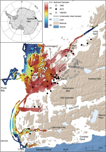
The study area, the Vestfold Hills, is one of the largest areas of ice-free coast in East Antarctica. They cover an area of 400 km2 and lie between 68°21'S and 68°41'S, and 77°49'E and 78°35'E. The coastline comprises small rocky islands, peninsulas and fjords (Fig. 1). Islands and hills on the mainland reach elevations of up to 60 m in the coastal zone rising to 156 m inland near the edge of the ice sheet. The Vestfold Hills are an Archean basement block surrounded by younger Precambrian metamorphic rocks to the north and south, and the Phanerozoic Prydz Bay Basin to the west (Stagg Reference Stagg1985, Collerson & Sheraton Reference Collerson and Sheraton1986). The eastern extent of the Vestfold Hills block is unknown because it is obscured by the ice sheet. This block forms an elevated plateau surrounded by deep troughs to the south and west, and probably deeper but more gently sloping bedrock to the north and east, though information on subice topography in these areas is limited.
Location of the Vestfold Hills, East Antarctica (inset). Shaded multibeam bathymetry map of the study area (2 m cell size grid, UTM Zone 43S projection). Hillshade illumination in this and subsequent figures is from the north-west (azimuth=315°, altitude=45°) unless otherwise stated. Location of underwater video transects and sediment samples acquired during the 2010 survey and historical sediment samples.

The Cenozoic geology and geomorphology of the Vestfold Hills have been extensively studied (Pickard Reference Pickard1982, Adamson & Pickard Reference Adamson and Pickard1986a, Reference Adamson and Pickard1986b, Fitzsimmons Reference Fitzsimmons1991, Reference Fitzsimmons1996, Gore et al. Reference Gore, Snape and Leishman2003, Quilty Reference Quilty2006). The overall picture is one of east–west to WSW–ENE trending valleys, floored with sediments and containing lakes. The area was overridden by ice advancing from the south-east during recent glaciations (Adamson & Pickard Reference Adamson and Pickard1986a). Pliocene marine sediments are preserved at Marine Plain (Quilty et al. Reference Quilty, Lirio and Jillett2000) and glacial deposits ranging from possible Pliocene age to late Pleistocene are present (Colhoun et al. Reference Colhoun, Kiernan, McConnell, Quilty, Fink, Murray-Wallace and Whitehead2010), though a detailed understanding of the area’s glacial history has yet to emerge. Holocene post-glacial raised beaches and lake deposits have been used to reconstruct a Holocene sea level curve post 8000 yr bp for the region (Peterson et al. Reference Peterson, Finlayson and Zhang1988, Zwartz et al. Reference Zwartz, Bird, Stone and Lambeck1998).
The climate is cold-polar with a mean maximum temperature of -7.4°C and a mean minimum temperature of -13°C (Bureau of Meteorology 2013). Snowfall is low with a mean annual precipitation of 70.5 mm water equivalent. The wind regime is dominated by strong flow from the north-east throughout the year, with occasional gentler sea breezes from the south-west in summer. The north-easterly winds blow from 067° (T) and dominate surface processes on land with ventifacts, wind scours, lee dunes, blizzard tails and snow banks all indicating NE–SW wind flow as the main surface-shaping agent (Pickard Reference Pickard1982). Mean wind speeds vary from 17 km hr-1 to 26 km hr-1, though maximum gusts of 206 km hr-1 have been recorded (Bureau of Meteorology 2013). Sea ice is present for most of the year. Freezing takes place intermittently from late February and break-out typically takes place in December. Break-out occurs progressively from south to north in response to prevailing winds from the north-east and the geometry of the coast. Vaz & Lennon (Reference Vaz and Lennon1996) described marine water masses and currents in the area. The Vestfold Hills coast is bathed by a water mass that has potential temperatures between -1.8°C and +2.1°C and salinities of 30.6–34.2 psu, and that flows from north to south with average velocities in the order of 0.015 m s-1. The tidal range is c. 1–2 m but velocities measured offshore from the study area were <0.01 m s-1. Primary productivity is high during spring and summer from both sea ice and open water phytoplankton, dropping to low during winter (Tucker Reference Tucker1988).
Methods
A geomorphic map of the study area was published by O’Brien et al. (Reference O’Brien, Stark, Johnstone, Smith and Riddle2012) that used hand-digitizing polygons based on visual inspection of a preliminary bathymetry grid. Here, final processed bathymetry and backscatter data are used. Automatic definition of geomorphic polygon boundaries was attempted to find more rigorous and reproducible polygon boundaries. This paper also includes descriptions of areas north and south of the Davis Station where limited multibeam swath data was collected (Fig. 1). Data coverage in these areas is insufficient to allow mapping of closed geomorphic polygons but is sufficient to provide additional insights into sedimentary processes in these areas.
Multibeam bathymetry and backscatter data
Multibeam bathymetric data were collected by Geoscience Australia from February to March 2010 using the Australian Antarctic Division workboat Howard Burton equipped with a Kongsberg EM 3002D 300 kHz dual head multibeam sonar system. Motion referencing and navigation data were collected using an Applanix Position and Orientation system (PosMV 320), coupled with a C-Nav Differential Global Positioning System (2050R), providing positional accuracy of ±0.2 m. An area of 42 km2 was surveyed with coverage of the swaths between 150 and 200% in the shallow waters closest to Davis Station (Fig. 1). Additional survey lines were run to Long Fjord in the north and to Crooked Fjord and the Sørsdal Glacier in the south.
The data were processed using Caris HIPS/SIPS v7.1 software. Initial processing of the multibeam data to account for tides and vessel motion (pitch, roll and heave), and to remove erroneous values and icebergs was completed during the survey. Final processing after the survey removed more complex artefacts and converted the data to mean sea level (MSL). Interpolated bathymetry surfaces were exported as a 2 m resolution grid for mapping purposes into ESRI ArcGIS 10.0 (Fig. 1). Bathymetric data are presented as plan and oblique shaded-relief images to differentiate the major sea floor landforms. Cross sections were taken through key sea floor features to show their dimensions.
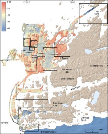
In addition to the bathymetric data, backscatter data were recorded by the multibeam sonar system. They were processed using CMST-GA MB Process v.8.11.02.1, a multibeam backscatter toolbox co-developed by Geoscience Australia and Centre for Marine Science and Technology (CMST), Curtin University for Technology. Backscatter intensity values were calculated following correction for transmission loss and area and removal of angular dependence (see Lucieer et al. Reference Lucieer, Hill, Barrett and Nichol2013 for further details). The final backscatter data were exported as a 2 m resolution grid. The data were colour coded and the resulting image is shown in Fig. 2.

The processed multibeam sonar bathymetric and backscatter data are published as data products and false-colour images. All of these data products are available for download from the Geoscience Australia website (http://www.ga.gov.au/metadata-gateway/metadata/record/gcat_76729).
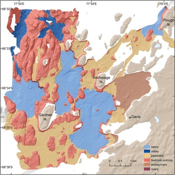
Six geomorphic units were identified and mapped within the central study area (Fig. 3). Mapping was undertaken in ArcGIS v10.0 (ESRI) using a combination of automatic extraction and manual digitization of polygons (see Finkl & Makowski Reference Finkl and Makowski2015). Automatic extraction of geomorphic units was completed using the Spatial Analyst toolbox in ArcGIS. The multibeam datasets include a large number of small-scale irregularities (a function of the high-resolution data) which tend to dominate derived attributes, making polygons overly complex. As the purpose of the mapping was to create a broad-scale map, lower resolution grids were created in order to remove some of the finer detail, thereby allowing smoother polygons to be created. The 2 m bathymetry and backscatter grids were reduced to 10 m resolution and a slope grid derived from the bathymetry grid. Depth, backscatter and slope contours were derived from at 1 m, 1 dB and 1° spacing, respectively. Raster Calculator was used to define cells according to the parameters outlined in Table I. The geomorphic units were then converted to polygons. The output from this automated process resulted in a large number of complex polygons (Supplemental Fig. 1 found at http://dx.doi.org/10.1017/S0954102015000371), including several undefined areas. The automated process highlighted some geomorphic features well (e.g. basins); however, other areas, particularly the rocky outcrops, were less well defined. The automatically extracted polygons were modified by hand to produce the final polygons to ensure that the final polygons reflected the surface morphology and seascape setting. The basins were smoothed first, mostly using the 3° slope or -21 dB backscatter contours. Rocky outcrops were smoothed next using the spacing of the slope contour (rather than a consistent slope contour) to define the change in slope, as well as the bedrock appearance of the sea bed in the bathymetry grid. The resulting interpreted geomorphic map (Fig. 3) contains simplified polygons that are morphologically coherent.
Map of submarine geomorphic units.

Datasets and parameters used to map the geomorphic features.

Underwater video
Underwater video data was used to ground-truth the geomorphic units and provide detail of sea floor features. Sixteen underwater video transects were surveyed in the study area using Geoscience Australia’s shallow-water Raytech towed-video system (Fig. 1). Full details of the collection and characterization of underwater video including the biota is published in Smith et al. (2015). The sea bed was characterized using the scheme of Anderson et al. (Reference Anderson, Cochrane, Roberts, Chezar and Hatcher2008) to record substrate composition (rock, boulder, cobble, pebble, sand, mud), bedforms (ripples, hummocks, iceberg scour features) and relief (smooth <1 m, moderate 1–3 m, high >3 m). The video was evaluated for 10 m segments, with a 10 m interval between each segment. All observations were entered into a Microsoft Excel spreadsheet via a programmable keyboard. The latitude and longitude of each observation was extracted from the workboat positioning data using the UTC time stamp overlay on the imagery.
The locations of the 643 discrete video observations were plotted in ArcGIS 10.0. Depth, backscatter intensity and slope values, as well as geomorphic unit, were extracted for each observation from the 10 m grids and combined with substrate, relief and bedform variables from the video characterization. A multivariate ordination technique was used to identify the major sources of variation in the data. Principal component analysis (PCA) was carried out using CANOCO v5.03 software (Ter Braak & Šmilauer Reference Ter Braak and Šmilauer2012) using depth, backscatter, slope, relief (flat, low 0.1–1 m, moderate 1–3 m, high >3 m), substrate (rock, boulder, cobble, pebble, gravel, sand, mud) and bedforms (ripples, hummocky, iceberg scour feature) as variables.
Sediment sampling
The sediment samples used come from a variety of studies. During the 2010 field season, 31 sediment samples were collected across the study area. Twenty-eight sediment samples were collected by divers from shallow-water sites close to Davis Station using a push corer (5 cm diameter). The top 5 cm of sediment was removed from the cores for analysis. The cores were kept upright and frozen at -20°C. A further three samples were collected from the workboat at deeper sites using a mini-shipek grab with a 30 cm wide mouth.
The sediment samples were analysed to determine the gravel, sand and mud content by washing sediment through a 2 mm sieve. The <2 mm fraction was also analysed for laser particle size using a Mastersizer 2000 Particle Analyzer. Homogenized sub-samples were analysed for organic matter (% OM) by loss on ignition following the procedure of Heiri et al. (Reference Heiri, Lotter and Lemcke2001). Carbonate content was determined using the carbonate ‘bomb’ gas evolution method (Muller & Gastner Reference Muller and Gastner1971), and biogenic silica was determined using the method of Mortlock & Froelich (Reference Mortlock and Froelich1989).
The sediment dataset was augmented by 37 sites collected from the study area in 1995. Of these records, several were recorded as no sample (primarily due to hard substrate) or small sample size, with 23 samples containing sufficient sample for grain-size analysis. Grain-size analysis of these samples was conducted by sieving samples into gravel, sand and mud fractions. Biogenic silica and carbonate content data was also available for 20 of these samples. Data on gravel-sand-mud content of onshore deposits collected by sieve analysis are available in a number of published papers (Hirvas et al. Reference Hirvas, Nenonen and Quilty1993, Gore et al. Reference Gore, Snape and Leishman2003, Colhoun et al. Reference Colhoun, Kiernan, McConnell, Quilty, Fink, Murray-Wallace and Whitehead2010) and an unpublished soil survey by Makarucha (Reference Makarucha1984). The locations of all sediment samples used in this study are shown in Fig. 1.
Geomorphic mapping
The multibeam bathymetry and backscatter data reveal the complexity and heterogeneity of the sea floor in the Vestfold Hills nearshore marine environment that has not been previously apparent (Figs 1 & 2). The inshore waters along the Vestfold Hills coast are very shallow (<10 m) increasing to c. 60 m within 5 km of the Davis Station coastline and to even deeper waters further offshore. At the mouths of Long and Crooked fjords, water depths increase rapidly to >200 m.
The blue tones in Fig. 2 represent low backscatter intensities and coincide with the distribution of acoustically non-reflective mud. Red tones indicate areas of high backscatter intensity, largely encompassing areas of exposed bedrock and large boulders. Yellow tones represent areas of intermediate backscatter intensity and are typically characterized by sandy sediment.
Six geomorphic features were identified and mapped from the multibeam datasets (Fig. 3).
Rocky outcrop
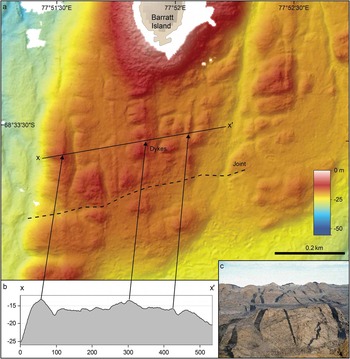
Bedrock outcrops form rounded hills and knolls with small and medium scale roughness. They vary from 50 m to 2 km across (e.g. in the north-west of the main study area). Multibeam images show geological features common to metamorphic terranes. For example, joint planes and faults are visible, as are dolerite dykes which form linear, rounded ridges standing slightly higher than the surrounding gneisses (Fig. 4a, b & c). Many bedrock outcrops have high backscatter (>-11 dB); however, some areas, where bedrock features are clearly displayed present low backscatter intensities indicating a thin sediment veneer.
a. Enlarged shaded bathymetry image of a bedrock outcrop south of Barratt Island. b. Cross-section of outcrop showing the location of north–south trending dykes. c. Photograph of dolerite dykes (in black) running for several tens of kilometres across the exposed bedrock in the adjacent Vestfold Hills.

Basins
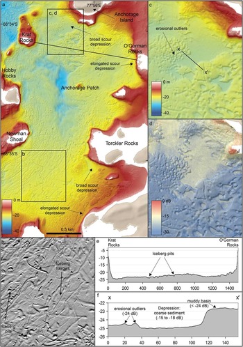
Basins are located between islands and bedrock outcrops, and are flat to slightly undulating and, as indicated by mostly low backscatter intensities (<21 dB), covered with sediment (Fig. Reference Barrie, Lewis, Parrott and Collins5a). Three main basins were identified in the study area, including two shallow basins (typically < 35 m) to the east and north-east of Gardner Island, and a deeper (>35 m) basin to the west of Gardner Island (Fig. 3). A basin in the northern part of the survey area near Plough Island was also partly mapped. Video transects and sediment samples in the basins indicate that they are typically floored with olive grey to green muddy fine sand to sandy mud. Ice keel scours are abundant (Fig. 5b & e).
a. Shaded bathymetry image of the inner basin east of Gardner Island showing elongated and broad scour depressions along the eastern margin. b. Enlarged shaded image showing iceberg pits and furrows. c. Enlarged shaded bathymetry image of a broad scour depression on the south-western margin of Anchorage Island. d. Enlarged shaded backscatter image of the broad scour depression showing coarser sediments in the depression compared to the surrounding muddy basin. e. Cross-section of the inner basin from Krat Rocks to O’Gorman Rocks, showing the relatively flat basin floor dissected by small iceberg pits and scours. f. Cross-section across the scour depression showing the steep slope separating the depression from the surrounding sea floor and backscatter intensity values for the depression and adjacent areas.

Pediments
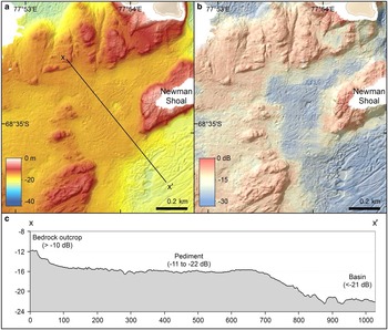
Between bedrock outcrops and sediment-floored depressions are broad areas that are flat to gently sloping which we classify as pediments based on their resemblance to pediments seen in many arid areas (Fig. Reference Bellec, Bøe, Rise, Slagstad, Longva and Dolan6a & b). The definition of pediment varies widely but is most commonly used for ‘gently sloping erosional surfaces of low relief, developed on bedrock’ (Dohrenwend & Parsons Reference Dohrenwend and Parsons2009). While the absence of sub-bottom profiler data means that we cannot confirm that the surfaces are cut on shallow bedrock, the morphology and location between or adjacent to bedrock hills are similar to many described pediments (Fig. 6a & c). Slopes are lower than the sides of rocky hills and the surfaces may undulate, possibly reflecting underlying near-surface bedrock. These surfaces mostly slope away from bedrock hills towards basins and commonly lack a clear step down to the basin level (Fig. 6c). Backscatter values are intermediate (typically -11 to -22 dB) which suggests sandy sediment. Iceberg scours are present in some of these areas but others lack apparent scours, possibly because the sediments are too coarse to retain well defined scour topography. Some pediment areas close to shore, e.g. north-east of Anchorage Island, contain boulder fields (see below).
a. Enlarged shaded bathymetry image of the pediment between Gardner Island and the inner basin. b. Enlarged shaded backscatter image of the same area showing the transition from hard (red) substrate to soft (blue) substrate. c. Cross-section showing the flat pediment surface and backscatter intensity values for the bedrock outcrop, pediment and basin.

Scarps
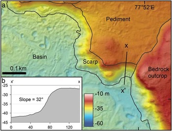
Scarps occur in several areas where steep slopes separate areas of level topography, such as pediment and basin areas. Such scarps separate ‘airport beach’ (informal name) embayment and the basin south of Anchorage Island, and form the eastern margin of the deeper basin west of Gardner Island (Fig. 7a). Scarps are differentiated from sides of bedrock hills because they represent distinctive steps between relatively flat surfaces (Fig. 7b). Where these areas adjoin bedrock hills, the boundary between the scarp and the bedrock hill slope was chosen as the steepest line directly downslope from the outermost edge of the bedrock hill to the basin or pediment below (Fig. 3).
a. Enlarged shaded bathymetry image of the scarp along the eastern margin of the deep basin west of Gardner Island, showing the boundaries of the scarp and surrounding geomorphic units. b. Cross-section of the scarp showing the steep slope between two relatively flat surfaces (pediment and basin).

Valleys
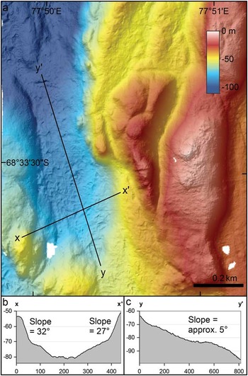
Valleys are present between some of the rocky hills, particularly in the deeper western part of the study area (Fig. 8a & b). They are differentiated from basins by being elongated with steeper sloping floors (Fig. 8c). Many valleys in the area are orientation north–south following the trend of faults and joints in the basement. Their substrate characteristics are relatively poorly known because video imagery was not collected in these areas.
a. Enlarged shaded bathymetry image of an elongated valley in the western part of the survey area. b. Cross-section of the valley showing the steep-sided valley walls. c. Longitudinal section of the valley showing the sloping valley floor.

Embayments
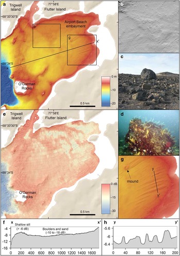
Some shallow areas <10 m deep, close to shore, are enclosed by peninsulas, islands and shallow sills therefore drifting ice does not scour the sea floor (e.g. Fig. 9a). These areas exhibit a relatively smooth sea floor but with abundant large boulders which are clearly visible in the multibeam grids (Fig. 9b). These boulders are <5 m in diameter and are similar to the large boulders found immediately onshore (Fig. 9c & d). The boundary of the embayment north of Davis Station was placed along a shallow ridge thought to act as a sill that extends from between Trigwell and Flutter islands in the north to near Davis Station in the south (Fig. 9e). The sea floor appearance and backscatter intensity was similar in other boulder field areas immediately to the west of the embayment boundary, as well as to the north of the embayment; however, the exclusion of icebergs by surrounding relief removes an important process of surface reworking from the embayment areas. In airport beach embayment, areas of sediment ripples evident in the underwater video, and linear sediment ridges, suggest current activity (Fig. 9g & h, see below).
a. Enlarged shaded bathymetry image of airport beach embayment. b. Enlarged image showing the presence of large (>4 m) individual boulders on the sea floor. c. Photograph of a large boulder onshore from the embayment. d. Underwater photograph of a large boulder inhabited by diverse benthic fauna in the shallow waters near Davis Station. e. Enlarged shaded backscatter image of airport beach embayment showing the predominantly hard substrate and areas of sand accumulation. f. Cross-section of the embayment showing the shallow sill used to delineate the embayment unit. g. Enlarged shaded bathymetry image of sand ribbons in airport beach embayment and a mound that is a possible pingo scar. h. Cross-section of the sand ribbons showing their irregular width and height.

Heidemann Bay is also enclosed, but was not mapped by multibeam sonar because of hazardous survey conditions.
Interpretation of sediment data
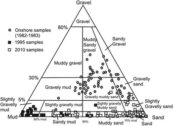
Sediment samples come from a range of sea floor environments, including basin, pediment and enclosed embayment locations. Most samples are muddy sand with some gravel to sandy mud (Fig. 10). Overall, gravel contents were low (<15%) and the only significant gravel contents (>5%) were found close to the shoreline and near the channels south of Gardner Island. There was a positive correlation between mud content, organic matter and biogenic silica (r 2 =0.75 and 0.70, respectively). Basin samples contained the highest proportion of muds, especially in the basin to the north-east of Gardner Island (Supplemental Fig. 2 found at http://dx.doi.org/10.1017/S0954102015000371). High mud contents were also recorded in a deep basin outside Laternula Inlet (supplementary Fig. 2). Basin samples contained an average of 9% organic matter and biogenic silica content of up to 22%.
Triplot of grain-size data of marine surface sediments from 1995 and 2010 surveys, and onshore sediments from 1982–83 survey. Grain-size classes from Folk (Reference Folk1954).

Pediment sample areas were mostly muddy sands, but sandy muds, sands and gravelly sands were also present. Pediment samples contained an average of 22% mud, 74% sand and 4% gravel. Organic matter and biogenic silica contents were lower than in the basins (2% and 5%, respectively). Overall, the carbonate content was low (average 1% in both basins and pediments); however, the sample taken adjacent to the channel features had a higher carbonate content (6%).
Compared to grain-size data from onshore sampling, the marine samples generally have less gravel and a higher proportion of mud (Fig. 10). The onshore datasets contain a significant proportion of glacial deposits; therefore, the observed difference in grain-size distributions can be explained by the marine samples containing sediment transported and deposited since deglaciation. The onshore samples most similar to those from offshore are those interpreted by Colhoun et al. (Reference Colhoun, Kiernan, McConnell, Quilty, Fink, Murray-Wallace and Whitehead2010) as marine deposits.
Correlation between geomorphic units and sea bed character
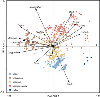
The PCA plot (Fig. 11) shows the relationship between physical sea bed variables and geomorphic units. The first two PCA axes cumulatively explained 41.9% of the total variation in the data. PCA axis 1, which alone accounted for 24.1% of the variation, was highly correlated with depth and longitude. PCA axis 2, which accounted for 17.8% of the variation in the data, was correlated with substrate (i.e. backscatter, mud and rock). Slope was correlated with both axes. Axis 1 represents, from left to right, gradient from shallow flat sea floor close to shore, to deeper and steeper sea floor further offshore. Axis 2 represents, from top to bottom, a gradient from steep rocky substrate to flat softer substrate. Coarse unconsolidated substrate (e.g. cobbles, pebbles, gravel) and iceberg scours did not display any strong trends with the geomorphologic units, with only short vectors in the PCA plot.
Principal component analysis (PCA) ordination plot showing the relationship between the physical variables, derived from the underwater video and multibeam data, and geomorphic units.

The position of the observations in the ordination space indicates the main similarities and differences in sea floor characteristics between the geomorphic units. The plot shows clear separation of basin, embayment, valley and rocky outcrop units. Basins had positive scores on axis 1 and negative scores on axis 2, indicating that they are deep, with muddy substrate and occur further offshore. Embayments had negative scores on axis 1 and mostly positive scores on axis 2, indicating that these areas are shallow, flat, hard and close to shore. Boulders, hummocky sea bed and ripples are common features in the embayments and also plotted in this direction. Observations from rocky outcrops dispersed widely in the PCA plot but had mostly positive scores on axis 1 and 2 indicating they have hard substrate and occur across a wide range of depths and with varying slopes. Observations from pediment areas lie in the centre of the plot, crossing both axes, and showing overlap with other units, indicating that they occur across a range of depths, are gently sloping and vary from hard and rocky to soft and sandy. This is consistent with them covering the transition from rocky outcrops to basins. Valleys had positive scores on axis 1 and mostly negative scores on axis 2, indicating that they occur in deeper water offshore, with relatively steep slopes and soft substrates. In summary, Fig. 11 shows a good separation between five geomorphic units which indicates that depth, backscatter and slope are useful for mapping geomorphic units with distinctive surface characteristics. Embayments do not appear separately in the PCA analysis because they are distinguished by their context in the topography rather than their surface character.
Deposits and sedimentary structures
A benefit of high-resolution multibeam bathymetry data is the ability to resolve sea floor sedimentary structures and deposits, such as bedforms, that provide insights into processes operating in the environment.
Iceberg scours
Iceberg scours are common across most of the areas where soft sediment is the main substrate. Scour shapes form a continuum from rounded sub-circular to elliptical depressions up to 45 m across (pits, Barrie et al. Reference Barrie, Lewis, Parrott and Collins1992; Fig. 5b) to long linear furrows as narrow as 4 m across and 385 m long (Fig. 5a & b). Almost all scours are <2 m deep with most <1 m deep. An inventory of scour widths and depths found no relationship between the two. Basin areas show overlapping scours at all scales. In the basin south of Anchorage Island, scours are oriented predominantly north–south with an arcuate trend convex to the east. Scours with pits at one end all have the pit at the northern or north-western end. A few east–west oriented scours are present.
On video transects, iceberg scours are harder to detect than might be expected given their visibility on the multibeam data. This largely reflects the subdued scour geometry. Most areas with scours visible on multibeam data, appear in video imagery as hummocky sea floor. Where visible on video, Vestfold Hills scours have rounded berms standing <1 m above the scour bed. Angular blocks of fractured, compacted sediment observed in berms of scours off Canada (Woodworth-Lynas et al. Reference Woodworth-Lynas, Josenhans, Barrie, Lewis and Parrott1991, Barrie et al. Reference Barrie, Lewis, Parrott and Collins1992) and George V Land shelf (Post et al. Reference Post, Beaman, O’Brien, Eléaume and Riddle2011) are not present.
During the survey, a small iceberg travelled slowly NE–SW across the area north of Anchorage Island. A video transect across the iceberg track revealed a fresh sea floor scour with rounded berms in light-coloured, probably sandy sediment, with a few boulders protruding. Also present within the scour were ridge-and-groove ‘microtopography’ (Woodworth-Lynas et al. Reference Woodworth-Lynas, Josenhans, Barrie, Lewis and Parrott1991) comprising sediment ridges c. 150 mm high and up to c. 300 mm across running parallel to the scour trough and the general direction of iceberg drift.
Channels
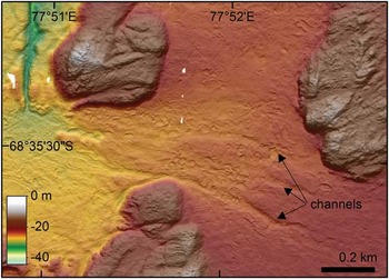
Narrow channels resembling drainage features cross the pediment area south of Gardner Island, running down slope normal to the prevailing current direction (Fig. 12). They have low sinuosity, are c. 30 m wide and 0.5–1 m deep, and their margins are modified by ice keel pits and scours.
Enlarged shaded bathymetry image of channels south of Gardner Island with hillshade illumination from the north (azimuth=0°, altitude=45°).

Boulder fields
The shallower areas in the east and north-east of the study area commonly show numerous boulders up to several meters in diameter standing above the sea floor or variably embedded in the substrate (e.g. airport beach embayment, Fig. 9b & d). The sea floor between the boulders is commonly sandy, with intermediate backscatter values. The multibeam data show irregular ridges and terraces c. 1–2 m above adjacent depressions. Boulder fields are also present in Heidemann Bay and in the shallow pediment area to the north of Anchorage Island. These areas are a continuation of a typical feature of the onshore south-western Vestfold Hills landscape (undulating valley fill of Gore et al. Reference Gore, Snape and Leishman2003, Fig. 9c).
Sand ribbons
In the south-eastern part of airport beach embayment, there is an area which features elongated ridges that are 50–300 m long and 5–30 m wide (Fig. 9a & g). Most trend towards 246° (T) though the most northerly pair of ridges trend 256° (T). The main group of 11 ridges varies in orientation by only a few degrees. The ridges are 0.2–0.5 m high at their highest (Fig. 9h). Their appearance suggests that they are sediment bodies overlying the boulder surfaces discussed above. This is reinforced by video transects which show them to comprise rippled sand, hence their designation as sand ribbons. Ripple orientations suggest sand transport roughly parallel to the ridges.
Mound with central depression
Within airport beach embayment is a single mound 50 m in diameter and 0.5 m high with a depression in the crest (Fig. 9a & g). Backscatter values are higher than adjacent sediments but similar to other parts of the embayment floored by boulder-rich sand. Two sand ribbons seem to have formed in the lee of the mound. The mound geometry is unlike bedrock outcrops protruding through the sediment cover in the embayment.
Scour depressions
Depressions occur in several places along the shallow (10–25 m) margins of the basins, immediately seaward of shallow rocky outcrops (Fig. 5a). Elongated depressions trend parallel to adjacent bedrock outcrops (e.g. depression next to O’Gorman Rocks, Fig. 5a) and broad depressions trend roughly perpendicular to the adjacent rocky outcrops. The elongated depressions are typically 0.5–1.0 m below the surrounding sediment, range from <30 m wide and <250 m in length and are often steep-sided.
Two larger depressions are found south-west of Anchorage Island (Fig. 5c & d) and west of Torckler Rocks (Fig. 5a), in water depths of 20–25 m and extending c. 250 m from the adjacent rocky outcrop (Fig. 5a). These broad depressions are characterized by coarser grained sediment (high backscatter intensity values c. -15 to -18 dB) than the surrounding finer grained sediment (low backscatter intensity <-24 dB) (Fig. 5d). They are typically 2 m below the surrounding fine-sediment sea floor and have SW–NE trending steep sides (Fig. 5f).
Within the broad depression south of Anchorage Island, a few curved, steep-sided ridges of material with low backscatter intensities are observed within the depressions with high backscatter (Fig. 5d). This relationship suggests that the ridges are eroded remnants of finer grained material overlying a coarser grained layer. Similar scour depressions with remnant ridges are present at the mouth of Heidemann Bay. Their appearance suggests that these depressions are probably areas of sediment erosion.
Areas beyond Davis Anchorage
Long Fjord
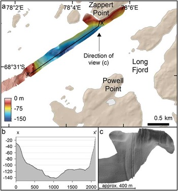
Long Fjord is a narrow inlet north of Davis Station where soundings from sea ice have recorded depths up to 222 m. Two multibeam survey lines were run obliquely across the fjord axis between Zappert and Powell points (Fig. 13a). Long Fjord has typical fjord morphology, i.e. a steep-sided valley with a mostly flat sea floor (Fig. 13b).
a. Enlarged shaded bathymetry image of the mouth of Long Fjord with hillshade illumination from the west (azimuth=270°, altitude=45°). b. Cross-section of the fjord entrance showing the steep sides of the fjord. c. Oblique perspective image of multibeam swath bathymetry within Long Fjord showing a series of gullies. The image is viewed from the south, illumination is from the west (azimuth=270°, altitude=25°) and vertical scale is 5x exaggerated.

The smooth sea floor suggests that most sedimentation is by settling from the water column but the fjord side adjacent to Zappert Point displays a set of gullies running downslope (Fig. 13c). Immediately above these gullies, but onshore, is a south-facing snow bank. Like many recurring snow banks in the Vestfold Hills, it contains enough debris, probably wind-blown material, to appear banded and dark. The gullies extend from the snow bank.
Ellis Fjord
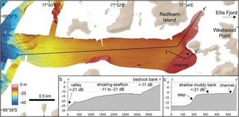
Ellis Fjord is one of the few places in Antarctica that receives stream flow from the continent with meltwater finding its way from the ice sheet edge via several lakes and narrow constrictions known as Ellis Narrows (Fig. 1). There are measured depths of >100 m in the inner fjord but the outer part of the fjord is shallow; therefore, multibeam data were collected in an area only 3.3 km inside the entrance (Fig. 14a). The entrance to Ellis Fjord has a partial sill composed of a rocky outcrop c. -16 to -18 m and a narrow valley with smooth floor c. -25 m MSL (Fig. 14a). The fjord floor shoals eastward to c. -15 to -12 m MSL near Redfern Island, where it shallows rapidly to only -2 m MSL (Fig. 14b & c) near Westwood Point.
a. Enlarged shaded bathymetry image of the entrance to Ellis Fjord with hillshade illumination from the north (azimuth=0°, altitude=45°). b. Cross-section showing the sea floor becoming shallower towards Westwood Point. c. Cross-section showing a step in the sea floor and narrow channel adjacent to the exposed bedrock.

Ellis Fjord has clusters of ice keel scours and large boulders, particularly in deeper water near the western end (Fig. 14a). The southern part of the fjord records intermediate backscatter intensity values <-21 dB with ice keel scours on its edge suggesting a bank of unconsolidated sediment. Its north-eastern margin is a narrow channel c. 0.4 m deep separating the bank from the exposed bedrock of Westwood Point.
Laternula Inlet
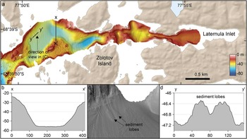
Laternula Inlet is parallel to Ellis Fjord and c. 3 km to the south. It is >60 m deep in places with a sinuous axis floored by smooth sediment bordered by rocky outcrops (Fig. 15a). The inlet cross-section is steep-sided, typical of fjords (Fig. 15b). Most of the inlet floor <30 m is smooth; however, two lobate sediment bodies 0.5 m high are present on the northern side (Fig. 15d). These lobes have long axes parallel to the slope and widen where the slope becomes less steep.
a. Enlarged shaded bathymetry image of sea floor to the east of Laternula Inlet with hillshade illumination from the west (azimuth=270°, altitude=45°). b. Cross-section of the fjord showing a steep-sided valley and smooth sea floor. c. Oblique perspective image of multibeam swath bathymetry showing two sediment lobes on the fjord walls, east of Laternula Inlet. The image is viewed from the south, illumination is from the south-west (azimuth=225°, altitude=18°) and vertical scale is 8x exaggerated. d. Cross-section of the sediment lobes.

Crooked Fjord
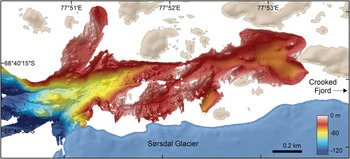
Crooked Fjord extends along the northern edge of the Sørsdal Glacier (Fig. 1). Its seaward end shows rugged sea floor with water depths approaching -350 m MSL (Fig. 16) and a number of shallow banks and islands. The multibeam image shows rocky outcrops with lineaments running parallel to the fjord axis and the glacier edge, suggesting that basement structural grain influences the position of the Sørsdal Glacier. The landward end of the fjord section surveyed displays smoother sea floor with depths of 30–40 m, but still with rocky outcrops and islands. Iceberg scours are present in water depths of c. -75 m MSL near the mouth of the fjord.
Enlarged shaded bathymetry image of sea floor to the east of Crooked Fjord.

Discussion
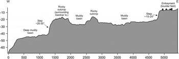
The overall distribution of geomorphic units and their elevation across the study area suggests that the landscape exhibits three general levels separated by abrupt ‘steps’ in the level of basins and pediments (Fig. 17). The eastern-most step marks the boundary between land areas, shallow embayments <10 m deep (airport beach embayment and Heidemann Bay) and shallow areas between islands. West of the step, depths of 18–30 m are typical, except around the steep sides of islands and rocky hills which approach the surface. The next step corresponds roughly to the western side of Gardner Island and represents a drop to >40 m water depth for basin and valley floors. The steps themselves are a series of arcuate scarps and slopes which are convex to the east and north-east. This geometry suggests they started as west-facing, north–south trending slopes which have retreated east in response to slope erosion. This, combined with the common north–south oriented faults and joints visible in bedrock outcrops (Figs 1 & 4a), would imply that north–south striking faults created the initial steps in bathymetry. The present indentations in the steps probably reflect changes in resistance of the rocks encountered. The eastern-most step in the landscape seems to mark the western limit of the boulder fields seen in the airport beach embayment and Heidemann Bay.
Cross-section across study area showing steps in the sea floor (location indicated in Fig. 2).

The undulating boulder-rich surface observed on land and in the multibeam data have been discussed by a number of authors. Hirvas et al. (Reference Hirvas, Nenonen and Quilty1993) suggested that the boulders were pushed to the surface by cryoturbation of underlying glacial till. However, they presented pebble fabrics from the underlying diamict which resemble unmodified, primary glacial till fabrics, suggesting minimal post-depositional disturbance. Franklin (Reference Franklin1997) suggested, based on onshore examples, that the boulder-rich ridges were beach ridges, invoking a combination of sea ice push and wave working. However, this proposed mechanism does not account for the wide distribution of large boulders.
The multibeam survey did not reveal any of the landforms commonly associated with glaciated surfaces such as flutes, megascale glacial lineations or drumlins. This accords with observation of the onshore Vestfold Hills (Adamson & Pickard Reference Adamson and Pickard1983). The NE–SW trending ridges, probably formed as moraines parallel to ice margin positions, are scattered across the Vestfold Hills but are mostly present south-east of Davis Station (Adamson & Pickard Reference Adamson and Pickard1983). Gore et al. (Reference Gore, Snape and Leishman2003) classified the glacial landforms preserved onshore as large debris ridges, small debris ridges, debris drapes and undulating valley fills. Of these landforms, the boulder fields detected by the multibeam survey resemble the debris drapes and undulating valley fills. The lack of streamlined bedforms and similar features probably reflects glaciation by ice frozen to its bed during the last period of glaciation of the Vestfold Hills. Therefore, we interpret the boulder fields and associated sand as deposits of cold-based ice that is known to produce boulder-rich sand deposits (Hambrey & Fitzsimmons Reference Hambrey and Fitzsimmons2010, Hambrey & Glasser Reference Hambrey and Glasser2012). The north-west limit of the boulder fields at the step in the landscape described above could represent the limit of the ice mass responsible for their deposition.
The mound with a depression in its crest within airport beach embayment is located within a boulder field making it likely that it is a glacial or periglacial feature. The shape of the mound and its central depression is similar to scars left by relict pingos (Pickard Reference Pickard1983). Consequently, it could be a pingo formed soon after deglaciation but before marine inundation, or it might also have formed as a small supraglacial lake deposit which was then lowered onto an ice core.
Iceberg scour geometry in the survey area can be understood in terms of factors described in studies from other regions (e.g. Hodgson et al. Reference Hodgson, Lever, Woodworth-Lynas and Lewis1988). The pits developed where an iceberg overturned, increased its draft and grounded (Hodgson et al. Reference Hodgson, Lever, Woodworth-Lynas and Lewis1988, Woodworth-Lynas et al. Reference Woodworth-Lynas, Josenhans, Barrie, Lewis and Parrott1991). The iceberg then remained stationary for a time, excavating a pit through small-scale movement and enhanced current velocities around the iceberg (Hodgson et al. Reference Hodgson, Lever, Woodworth-Lynas and Lewis1988). Ablation then reduced the iceberg size, it then either floated or the keel protruded less into the substrate, reducing resistance, so it then moved across the bed, producing examples where a pit has a scour attached. Around the Vestfold Hills, such pits have the accompanying scour trending south or south-west indicating that most icebergs drift with the local ocean current and prevailing north-east winds (Vaz & Lennon Reference Vaz and Lennon1996). The lesser numbers of east–west scours probably indicate small icebergs or sea ice keels influenced by tidal currents or the occasional south-west sea breeze in summer. The arcuate trend through the Anchorage basin also reflects local oceanographic flow.
The subdued, rounded topography of the scours, the rarity of clear ridge-and-groove microtopography and the absence of angular blocks of disturbed sediment in berms probably reflects the properties of the sea floor sediments around Davis. Hodgson et al. (Reference Hodgson, Lever, Woodworth-Lynas and Lewis1988) surveying iceberg scours on the Canadian margin found that sediment with high sand content and low cohesion did not produce steep berm slopes or angular blocks of sediment in the scour surcharge. The sediments around Davis likewise have low cohesion, and therefore, do not produce steep slopes or angular blocks.
A number of features suggest erosion and deposition by current activity under conditions of low sediment supply. As there have been no current meter deployments in airport beach embayment, observations of sedimentary structures must be used to understand the origins of these features. The orientation of most of the ribbons parallel to the prevailing north-east (from 067° T) wind suggests that water is driven south-west along the embayment, entraining sand provided by the beach and snow patch run-off at the north-east shore of the embayment. However, the ripples do not show clear asymmetry on the video images. The video transect north-west of the sand ribbons also shows rippled sand but it also shows a large boulder with scouring on the south-west (up-current side) and a tail of rippled sand on the north-east (lee) side indicating current flowing from the south-west towards the north-east. This suggests that significant bottom sediment transport occurs when occasional south-west winds drive water into the embayment. This water then flows out along the south-east side of the embayment, forming the observed sand ribbons.
Published relative sea level estimates for the area suggest that, if the channels south of Gardener Island formed subaerialy, they have been underwater and subjected to iceberg modification for >12 000 years (Zwartz et al. Reference Zwartz, Bird, Stone and Lambeck1998, Nakada et al. Reference Nakada, Kimura, Okuno, Moriwaki, Miura and Maemoku2000). Their persistence suggests that they are maintained by episodic bottom currents flowing downslope and roughly normal to the prevailing ocean currents. Thus, both the channels and sand ribbons suggest that wind-driven coastal down-welling is a significant, though episodic, process on the Vestfold Hills coast.
The gullies in Long Fjord and sediment lobes in Laternula Inlet indicate that gravity-driven processes are active on steep slopes. The Long Fjord gullies are immediately downslope from a perennial, sediment-laden snow bank, suggesting that they are produced by sediment-charged meltwater from the snow bank forming turbidity currents capable of eroding the sea floor. The Laternula Inlet sediment lobes are probably deposits of sediment gravity flows. They lack blocks and masses of partly disaggregated material expected in flows of cohesive material, rather their lobate form is more like deposits of highly concentrated sand-water flows (Carter Reference Carter1975).
Several basin areas contain eroded areas resembling shelf scour depressions. Proposed mechanisms for the formation of these depressions include tidal scour (Bellec et al. Reference Bellec, Bøe, Rise, Slagstad, Longva and Dolan2010), cross-shore currents (Cacchione et al. Reference Cacchione, Drake, Grant and Tate1984), storm-generated down-welling (Garnaud et al. Reference Garnaud, Lesueur and Garlan2005), and along-shore currents. It is likely that scouring is induced by strong flows steered and concentrated by the bedrock outcrops across the area (Cacchione et al. Reference Cacchione, Drake, Grant and Tate1984). No current measurements are available on the inner shelf within the domain of the scour depressions; however, it is reasonable to assume that enhanced bottom stresses produced by focusing of local currents are capable of re-suspending and transporting the surficial fine sediment (Cacchione et al. Reference Cacchione, Drake, Grant and Tate1984). The scour depressions at the seaward end of Heidemann Bay may be of tidal origin as they are sheltered from the main north–south currents.
The airport beach embayment sand ribbons and channels on the pediment south of Gardener Island are probably the result of wind-driven down-welling currents. The scour depression between islands and bedrock hills are more probably formed by constriction of oceanographic currents by topography. Published accounts of modern sediment transport in the Vestfold Hills have emphasized wind erosion and transport (Pickard Reference Pickard1982, Adamson & Pickard Reference Adamson and Pickard1986b), fluvial transport derived from snow and ice margin melt (Fitzsimmons Reference Fitzsimmons1991), subaerial mass movement (Fitzsimmons Reference Fitzsimmons1996) and wave reworking of shoreline deposits (Peterson et al. Reference Peterson, Finlayson and Zhang1988). Our multibeam data show that wind-driven and oceanographic currents also play a role in transporting sediment. Ice keel scouring must also enhance sediment mobility by dislodging fine material and making it more susceptible to geostrophic or tidal currents. The data from steep fjords shows evidence of mass transport processes redistributing sediment from the shoreline into deep water in the form of turbidity current gullies and lobate mass transport deposits. The overall impression of the area is that it is a landscape covered by slow-moving glacial ice which has been modified by marine processes after deglaciation. This contrasts with Prydz Bay to the west where fast-flowing ice streams have been a feature through the Cenozoic (O’Brien et al. Reference O’Brien, Goodwin, Forsberg, Cooper and Whitehead2007). This adds to a picture of glaciation of the Antarctic coast involving fast-flowing outlet glaciers in deep troughs and slow-moving cold ice or even unglaciated areas in areas of higher elevation (Mackintosh et al. Reference Mackintosh, Verleyen, O’Brien, White, Jones, McKay, Dunbar, Gore, Fink, Post, Miura, Leventer, Goodwin, Hodgson, Lilly, Crosta, Golledge, Wagner, Berg, van Ommen, Zwartz, Roberts, Vyverman and Masse2014).
Conclusions
Multibeam sonar, underwater video and sediment sampling allow the mapping of geomorphic units and provide insights into sea floor processes and environments in the nearshore areas of the Vestfold Hills. Mapped units include rocky outcrops, sediment-floored basins, pediments, valleys, scarps and embayments protected from scouring by floating ice. Iceberg scours are plentiful, and sand ribbons and sea floor channels indicate significant sediment movement by marine currents. Steep-sided valleys show features formed by sediment gravity flows. Features formed by subglacial deposition are not common with undulating, boulder-rich sand units representing deposition by cold-based ice. The geomorphic map presents an integrated view of the sea floor that can be used to understand the distribution of benthic habitats, the action of sea floor sedimentary processes and provides pointers to the past history of the area. Identification of features produced by sediment erosion and deposition point to processes that shape the benthic environment but which have not been observed directly to date.
Acknowledgements
We thank Ian Atkinson (GA), Ross Bowden, Dean Forrest, Jade Paddison and Steven Swanson (RAN) for survey assistance, Michele Spinoccia, Olivia Wilson and Dr Justy Siwabessy (GA) for processing the multibeam data, and Dr Alix Post (GA) for assisting with interpretation and analysis of the underwater video data. This research was part of Australian Antarctic Science (AAS) Project 2201 – Natural Variability and Human Induced Change on Antarctic Nearshore Marine Benthic Communities (CI: Martin Riddle). The bathymetry data collection was part of Australian Antarctic Division non-science Project 3259 – Hydrographic Charting of Antarctic Waters. Dr Scott Nichol, Dr Kim Picard, Prof Mike Hambrey and an anonymous reviewer are thanked for their review of this manuscript. This paper is published with the permission of the Chief Executive Officer, Geoscience Australia.
©Commonwealth of Australia (Geoscience Australia) 2015.
Author contribution
Philip E. O’Brien: survey design, multibeam survey operation, video data collection, data processing, geomorphic mapping and interpretation, text and paper preparation. Jodie Smith: backscatter and automated geomorphic mapping and interpretation, PCA analysis, text and figure preparation. Jonathan Stark: sediment and video sampling, sample analysis and interpretation. Glenn Johnston: sediment and video sampling, sample analysis and interpretation. Martin Riddle: survey design and interpretation. Denis Franklin: sediment sampling, analysis and interpretation.
Supplementary Material
Two supplemental figures will be found at http://dx.doi.org/10.1017/S0954102015000371.