





Highlights
What is already known?
-
• Selective reporting of primary study results can distort the findings from meta-analyses.
-
• In many fields of application, meta-analyses include primary studies providing multiple, statistically dependent effect size estimates.
-
• Step-function selection models are a theoretically appealing tool for correcting bias from selective reporting, but these models were developed for meta-analyses that include only one effect size estimate per study.
What is new?
-
• We examine strategies for estimating step-function selection models in meta-analyses with dependent effect sizes.
-
• We report a large simulation study demonstrating that step-function models can be estimated using penalized maximum likelihood methods, combined with bootstrapping techniques to account for dependent effect size estimates.
Potential impact for RSM readers
-
• The proposed estimation methods can be applied to adjust for selective reporting of study results in meta-analyses with 30 or more studies that include dependent effect sizes.
-
• This strategy complements other existing methods for examining selective reporting bias in meta-analyses with dependent effect sizes.
1 Estimation and inference for step-function selection models in meta-analysis with dependent effects
The validity of conclusions from meta-analytic syntheses depends critically on the reporting practices of researchers, journal editors, and peer reviewers. If the findings accessible to meta-analysts are not a representative record of the research that has been conducted on a topic, then meta-analytic summaries may be systematically biased.Reference Rothstein, Sutton, Borenstein, Rothstein, Sutton and Borenstein 1 Of particular concern is the possibility that results from primary studies are selectively reported in ways that distort the evidence available for synthesis, such as by reporting findings that are statistically significant but omitting findings that are null or not consistent with researchers’ hypotheses.Reference Greenwald 2 , Reference Sutton 3
Selective reporting practices can occur at the level of the entire study or at the level of a specific finding within a study. At the study level, publication bias occurs when full study reports are withheld from public availability as a function of some aspect of their findings.Reference Sutton 3 , Reference Dwan, Gamble, Williamson and Kirkham 4 Reports with statistical conclusions that support research hypotheses may be more likely to be published than those that do not. At the level of the individual finding, a study that clears the hurdle of publication might still include results for only a subset of analyses conducted or outcome measures examined, leading to outcome reporting bias.Reference Dwan, Gamble, Williamson and Kirkham 4 , Reference Williamson, Gamble, Altman and Hutton 5
Evidence from medical, educational, and social sciences provides indications of the prevalence of selective reporting. For example, studies have found that statistically significant outcomes were 2.4–4.7 times more likely to be published than non-significant outcomes in the medical sciencesReference Chan, Hróbjartsson, Haahr, Gøtzsche and Altman 6 and 2.4 times more likely in education.Reference Pigott, Valentine, Polanin, Williams and Canada 7 Studies examining various fields, including clinical trials of antipsychotics,Reference Lancee, Lemmens, Kahn, Vinkers and Luykx 8 psychology research,Reference Franco, Malhotra and Simonovits 9 , Reference van Aert, Wicherts and van Assen 10 management science,Reference O’Boyle, Banks and Gonzalez-Mulé 11 economics, and environmental sciences,Reference Bartoš, Maier and Wagenmakers 12 have found widespread selective outcome reporting on the basis of statistical significance.
Because selective reporting is of such central concern for meta-analysis, a wide range of statistical tools have been developed for detecting its presence and reducing the biases it creates.Reference Rothstein, Sutton, Borenstein, Rothstein, Sutton and Borenstein
1
,
Reference Marks-Anglin and Chen
13
One common graphical diagnostic is the funnel plot, a simple scatterplot of effect size estimates versus a measure of their precision.Reference Sterne, Becker, Egger, Rothstein, Sutton and Borenstein
14
Widely used statistical diagnostics include the rank correlation testReference Begg and Mazumdar
15
; Egger’s regression testReference Egger, Smith, Schneider and Minder
16
; the trim-and-fill adjustmentReference Duval and Tweedie
17
; and various regression adjustment methods, including the precision effect test (PET), precision effect estimate with standard error (PEESE), PET–PEESE technique,Reference Stanley and Doucouliagos
18
and endogenous kink meta-regression.Reference Bom and Rachinger
19
Another class of methods for assessing and correcting selective reporting are
$p$
 -value selection models, which build on summary meta-analysis or meta-regression models by making explicit assumptions about how the probability that an effect size estimate is reported relates to the sign and statistical significance level of the effect. Building on earlier proposals,Reference Hedges
20
–
Reference Dear and Begg
22
Vevea and Hedges proposed step-function models where the selection function is piece-wise constant, with steps at fixed significance thresholds.Reference Hedges
23
,
Reference Vevea and Hedges
24
The step-function model captures simple but plausible forms of selective reporting, such as shifts in selection probability at the psychologically salient thresholds of
$p=0.05$
 or
$p=0.01$
 .Reference Greenwald
2
,
Reference Nelson, Rosenthal and Rosnow
25
–
Reference Rosenthal and Gaito
27
Step-function selection models have several advantages over other available methods for diagnosing and adjusting for selective reporting bias. First, they are generative models with parameters that directly describe the selective reporting process, making them more interpretable than regression adjustments for small-study effects, which are agnostic with respect to the specific mechanism of selective reporting. Second, they can incorporate both discrete and continuous moderators, enabling one to distinguish between selective reporting bias and systematic differences in effect size that can be predicted by primary study characteristics. Third, findings from simulations indicate that simple forms of step-function models outperform alternative bias adjustment methods when effect sizes are heterogeneous because they allow for the inclusion of a random-effect term.Reference Carter, Schönbrodt, Gervais and Hilgard 28 – Reference Hong and Reed 30
Step-function models also have drawbacks that should be considered. Notably, they are more complex—and perhaps less intuitive—than regression adjustments or trim-and-fill. The thresholds in the step function must be chosen a priori, and so may not correspond to the true selective reporting process. Furthermore, the models are built on the assumption that the selection process is homogeneous across study features other than statistical significance, such as study size or funding status. Step-function models also require a larger number of effect sizes for accurate estimation of the model parameters, particularly when a more complex (i.e., multiple-step) selection process is assumed. Despite these complexities, the plausible selective reporting process expressed by the step-function model, coupled with its demonstrated performance in past simulations,Reference Carter, Schönbrodt, Gervais and Hilgard 28 , Reference McShane, Böckenholt and Hansen 31 makes it a promising approach for analyzing and correcting the bias arising from selective reporting.
1.1 Dependent effect sizes
The vast majority of the work on selective reporting has focused on methods appropriate for relatively simple summary meta-analyses in which each included study contributes a single independent effect size estimate. This presents a problem for syntheses in education, psychology, and many other areas, where meta-analyses routinely include studies with multiple, dependent effect sizes. Effect size dependencies occur when multiple effect sizes are extracted from the same sample, resulting in statistically dependent estimates. Dependent effect size estimates commonly occur (1) when multiple outcome measures are collected on the same sample; (2) when the same sample is measured over multiple time points; or (3) when multiple treatment groups are compared to the same control group.Reference Becker, Brown and Tinsley 32 These phenomena lead to estimates with correlated sampling errors, or what we refer to as a correlated effects dependence structure. Dependence can also arise when effect sizes are extracted from multiple samples involving the same operational features, such as multiple studies conducted by the same research group, leading to a hierarchical effects dependence structure.Reference Hedges, Tipton and Johnson 33
Effect size dependencies are very common in social science synthesis, as well as in other research areas.Reference Wu, Duan, Reed and Tipton 34 For example, for the more than 1,000 educational intervention studies reviewed by the What Works Clearinghouse since 2017, 73% included more than one intervention effect estimate, with a median of four effect sizes per study (WWC, 2020). Surveys of systematic reviews on topics in psychology,Reference Tipton, Pustejovsky and Ahmadi 35 education,Reference Pellegrini, Pigott, Chubb, Pruitt and Scarbrough 36 environmental sciences,Reference Nakagawa, Yang, Macartney, Spake and Lagisz 37 and neurobiologyReference Yang, Macleod, Pan, Lagisz and Nakagawa 38 have also documented a high prevalence of dependent effect sizes. Thus, multiple effects are often the norm rather than the exception.
Meta-analysts now have access to an array of methods for summarizing and modeling dependent effect sizes. For hierarchical effects dependence, analysts can apply multilevel meta-analytic models that provide estimates of effect heterogeneity at each of several levels.Reference Konstantopoulos 39 , Reference van den Noortgate, López-López, Marín-Martínez and Sánchez-Meca 40 For some specific forms of correlated effects dependence such as studies with multiple treatment groups or factorial treatment structure, multivariate meta-analysis methods are available that treat findings from a given study as a vector with distinct dimensions.Reference Jackson, Riley and White 41 – Reference Van Houwelingen, Arends and Stijnen 43 However, many instances of dependent effects involve both correlated and hierarchical effects structure; in other instances, the multiple findings reported in some studies do not have a regular dimensional structure; and commonly, the information needed to estimate the correlation structure of effect size estimates is not available in primary study reports.Reference Pellegrini, Pigott, Chubb, Pruitt and Scarbrough 36 , Reference Pustejovsky and Tipton 44
In circumstances where the exact dependence structure of effects does not fit neatly into multilevel or multivariate models, a technique known as robust variance estimation (RVE)Reference Hedges, Tipton and Johnson 33 has proven to be an attractive strategy. RVE is useful because it provides a means to assess uncertainty in model parameter estimates that does not rely on strong assumptions about the exact dependence structure of the effect size estimates. Instead, RVE involves specifying a tentative working model for the dependence structure, but calculating standard errors, hypothesis tests, and confidence intervals (CIs) using sandwich estimators that do not require the working model to be correct. RVE can also augment other modeling techniques by specifying working models that capture multiple forms of dependence, as in the correlated-and-hierarchical effects (CHE) model proposed by Pustejovsky and Tipton, which allows for correlated effect estimates as well as heterogeneity of true effects both within and across studies.Reference Pustejovsky and Tipton 44 A closely related strategy is to use bootstrap re-sampling to approximate the distribution of test statistics.Reference Joshi, Pustejovsky and Beretvas 45 However, extant developments in RVE and bootstrapping methods are limited to summary meta-analysis and meta-regression models. Applications to selection models remain to be explored.
1.2 Investigating selective reporting with dependent effect sizes
Methodologists have only recently begun to examine selective reporting detection or bias-correction methods in meta-analysis involving dependent effect sizes. Mathur and VanderWeele proposed a sensitivity analysis based on the simplest possible form of the step-function selection model, with effect size dependence handled using RVE.Reference Mathur and VanderWeele 46 This sensitivity analysis provides an estimate of the average effect size after correcting for selection with a single, threshold statistical significance level, where the maximum strength of selection is pre-specified by the analyst. This approach is premised on an assumed degree of selective reporting; thus, it does not estimate the strength of selection, nor does it have extensions to more complex step functions with multiple thresholds. Another alternative is to use a regression test for small-study effects, or association between effect sizes and standard errors, combined with RVE or multilevel meta-analysis to handle dependent effect sizes.Reference Fernández-Castilla, Declercq, Jamshidi, Beretvas, Onghena and van den 47 , Reference Rodgers and Pustejovsky 48 This method has limited power to detect selective reporting under common meta-analytic scenarios.Reference Rodgers and Pustejovsky 48 It also has the same limitations as univariate Egger’s regression, in that it tests for a pattern of small-study effects, which could have causes other than selective reporting.Reference Sterne, Sutton and Ioannidis 49
Chen and Pustejovsky reviewed a range of existing techniques for estimating average effect sizes in the presence of selective reporting and dependent effect sizes.Reference Chen and Pustejovsky
50
They also proposed adaptations of several existing methods that can be formulated as meta-regressions, such as PET/PEESE and the endogenous kink method, with dependence addressed using a particular working model combined with RVE. In an extensive simulation study, they examined the performance of proposed adaptations alongside existing methods that ignore effect size dependence, under scenarios where the selective reporting process was consistent with a one-step (
${\alpha}_1=0.025$
 ) or two-step selection model (
${\alpha}_1=0.025$
 and
${\alpha}_2=0.500$
 ). Although no single bias-correction method performed best across all conditions examined, simple forms of the step-function selection model emerged as strong candidates. Across a wide range of conditions, one-step and two-step selection models yielded average effect size estimates with low bias that were usually more accurate than alternative bias-adjusted estimators. The strong performance of step-function models may be explained by the alignment between the assumptions of the step-function model and the mechanism used to introduce selective reporting in the data-generating process of the simulations. However, because the step-function models involve the assumption that all effect sizes are independent, CIs generated from the selection models did not have accurate coverage. These findings underscore the need to further develop selection models that can account for dependent effect sizes.
To address this need, we investigate how to estimate selection models and provide valid assessments of uncertainty in parameter estimates for meta-analyses that involve dependent effect sizes. In applying selection models to datasets involving dependent effects, we propose to model the marginal distribution of the effect size estimates rather than the joint distribution of the dependent effects within each study. This means we model each estimate considered as a single observation, without explicitly accounting for its dependence on other effect sizes from the same study. To account for dependence, we consider cluster-robust variance estimation and clustered bootstrap inference methods that allow for dependent observations even though it is not directly modeled. This strategy does have the limitation that the model parameter estimates pertain only to the marginal distribution and do not distinguish between selective publication of full studies versus selective reporting of individual outcomes.
Despite this limitation, we believe that the strategy of modeling the marginal distribution is worth pursuing for at least three reasons. First, this strategy captures a plausible form of selection, in which reporting is influenced by the significance level of individual effect size estimates. In contrast, developing a multivariate selection model would require specifying assumptions about the probability that each of many possible subsets of effect sizes is reported or censored. Little past work on reporting practices has considered reporting of multiple findings within a study, so there is currently little empirical basis to support assumptions about multivariate selection processes.Footnote i Moreover, it seems reasonable to assume that the statistical significance level of individual effect size estimates would still be a major consideration in more nuanced, multivariate selection models.
Second, focusing on the marginal distribution allows for computational tractability, whereas fitting even quite basic multivariate models would require computing selection probabilities over high-dimensional spaces of possible outcomes. Recent work attempting to implement multivariate selection models in a Bayesian framework noted that such models become computationally intractable when primary studies include more than three dependent effect sizes.Reference Bartoš, Maier and Wagenmakers 52
Third, the marginal modeling strategy has several precedents within the meta-analytic and broader statistical literature. For instance, generalized estimating equations often use a “working independence” structure to estimate parameters in longitudinal data without requiring specification of the joint distribution of the repeated measurements.Reference Liang and Zeger 53 Similarly, the unrestricted weighted least squares approach for meta-regression relies on marginal modeling to provide a simpler alternative to complex hierarchical structures,Reference Stanley and Doucouliagos 54 and pseudo-likelihood estimators for multivariate meta-analysis simplify the problem by focusing on the marginal likelihoods of individual variates.Reference Chen, Hong and Riley 55 Thus, we focus on developing marginal step-function selection models as a practical and feasible tool, which could also serve as a building block for more complex multivariate models.
The remainder of the article is organized as follows. In the next section, we describe the marginal step-function selection model and detail two different strategies for estimating model parameters: one using penalized maximum likelihood estimation methods and a novel strategy based on a re-weighted random-effects model with inverse probability of selection weights. We also describe extensions of RVE and bootstrap re-sampling techniques to assess uncertainty in selection model parameter estimates. In the following section, we provide an empirical example that illustrates the methods by re-analyzing data from a previously reported meta-analysis. In subsequent sections, we describe the methods and results from a simulation study that evaluates the performance of point estimators and CIs across a wide range of meta-analytic conditions involving a single-step selection process. In the final section, we discuss findings, limitations, and implications for practice.
2 Models and estimation methods
Step-function selection models involve two components.Reference Hedges, Vevea, Rothstein, Sutton and Borenstein 56 The first component, which we call the evidence-generating process, involves assumptions about the distribution of effect size estimates prior to selective reporting. This component is usually a random-effects model or meta-regression model. The second component, which we call the selection process, involves assumptions about how effect size estimates come to be observed and therefore available for inclusion in the meta-analysis. Combining these components leads to a model for the distribution of observed effect size estimates.
We will use the following notation to describe the model and estimation methods. Let
$\Phi \!\! \left(\right)$
 denote the standard normal cumulative distribution function and
$\phi \!\! \left(\right)$
 denote the standard normal density function. Consider a meta-analytic sample consisting of
$J$
 studies, in which study
$j$
 reports
${k}_j$
 effect size estimates. Let
${y}_{ij}$
 denote observed effect size estimate
$i$
 from study
$j$
 , defined so that positive values are consistent with theoretical expectations. Each estimate is accompanied by a standard error
${\sigma}_{ij}$
 and corresponding one-sided
$p$
 -value
${p}_{ij}=1-\Phi ({y}_{ij}/{\sigma}_{ij})$
 , where the one-sided
$p$
 -value is defined with respect to the null hypothesis that the effect is less than or equal to zero and the alternative hypothesis that the effect is positive. Let
${\mathbf{x}}_{ij}$
 be a
$1\times x$
 row vector of predictors that encode characteristics of the effect sizes, samples, or study procedures.
2.1 Evidence-generating process
We consider an evidence-generating process based on a conventional meta-regression model. Let
${Y}^{\ast }$
 denote an effect size estimate that has been generated from primary study data but might or might not be reported; let
${\sigma}^{\ast }$
 ,
${p}^{\ast }$
 , and
${\mathbf{x}}^{\ast }$
 denote the corresponding standard error, one-sided
$p$
 -value, and predictor vector.Footnote
ii
The evidence-generating process can then be expressed as

where
$\boldsymbol{\beta}$
 is an
$x\times 1$
 vector of regression coefficients that relate the predictors to average effect size and
${\tau}^2$
 is the variance of the distribution of effect size parameters. This random-effects meta-regression treats each observed effect size as if it were independent, even though the data may include multiple, statistically dependent effect size estimates generated from the same sample. As a result, the regression coefficients
$\boldsymbol{\beta}$
 describe the overall expected effect size (given the predictors) and the variance parameter
${\tau}^2$
 describes the heterogeneity of the marginal effect size distribution, rather than decomposing the heterogeneity into within-study and between-study components.
2.2 Selection process
At a general level, a
$p$
 -value selection process is defined by a selection function, which specifies the probability that an effect size estimate is reported given its
$p$
 -value. Letting
$O$
 be an indicator for whether the effect size estimate
${Y}^{\ast }$
 is observed, the selection process involves the assumption that
$\Pr \left(O=1\;|\;{p}^{\ast}\right)$
 is proportional to a function
$w\left({p}^{\ast };\boldsymbol{\lambda} \right)$
 that maps
$p$
 -values in the interval
$\left[0,1\right]$
 to strictly positive weights based upon an unknown
$H\times 1$
 parameter vector
$\boldsymbol{\lambda} =\left({\lambda}_1,\dots, {\lambda}_H\right)$
 .
Vevea and HedgesReference Vevea and Hedges
24
described a random-effects meta-regression model where selection weights vary depending on a set of pre-specified thresholds for the one-sided
$p$
 -value, chosen based on conventional, psychologically salient cut-offs for judging statistical significance. Let
${\alpha}_1,\dots, {\alpha}_H$
 be a set of thresholds for the one-sided p-values, and set
${\alpha}_0=0$
 ,
${\alpha}_{H+1}=1$
 , and
${\lambda}_0=1$
 . A step-function selection model can be written as

or equivalently as

Setting
${\lambda}_0=1$
 is necessary for identification because the absolute probabilities of selection cannot be estimated. The remaining parameters are therefore interpreted as relative probabilities of selection, compared to the selection probability of a finding with
${p}^{\ast}\le {\alpha}_1$
 .
In practice, meta-analysts will often use only a small number of steps in the selection model. One common choice is the three-parameter selection model, which has a single step at
${\alpha}_1=0.025$
 , as depicted in Figure 1a. With this choice of threshold, positive effects that are statistically significant at the two-sided level of
$p<0.05$
 have a different probability of selection than effects that are not statistically significant or not in the anticipated direction. Another possibility is to use two steps at
${\alpha}_1=0.025$
 and
${\alpha}_2=0.500$
 , which allows for different probabilities of selection for effects that are positive but not statistically significant and effects that are in the opposite of the expected direction, as depicted in Figure 1b.
Examples of step functions.

Figure 1. Long description
Panel a is titled One-step selection with lambda sub 1 equals 0.4. The y-axis is selection probability from 0.00 to 1.00. The x-axis is p-value one-sided from 0.0 to 1.0. A red shaded area begins at a selection probability of 1.00. At a p-value of 0.025, indicated by a vertical dashed line, the probability drops sharply to 0.40 and remains constant across the rest of the x-axis.
Panel b is titled Two-step selection with lambda sub 1 equals 0.4, lambda sub 2 equals 0.2. The axes are identical to panel a. A purple shaded area begins at a selection probability of 1.00. At a p-value of 0.025, indicated by a vertical dashed line, the probability drops to 0.40. At a p-value of 0.500, indicated by a second vertical dashed line, the probability drops again to 0.20 and remains constant for the remainder of the x-axis.
2.3 Distribution of observed effect size estimates
Combining the assumptions of the evidence-generating process and the selection process leads to a model for an observed effect size estimate. The marginal distribution of an observed effect size estimate
$Y$
 with standard error
$\sigma$
 is equivalent to the distribution of
${Y}^{\ast }$
 given that
$O=1$
 , with density function

where

If
$w\left(y,\sigma; \boldsymbol{\lambda} \right)=1$
 for all possible
$y$
 , then there is no selective reporting,
$A\left(\mathbf{x},\sigma; \boldsymbol{\beta}, {\tau}^2,\boldsymbol{\lambda} \right)=1$
 , and the density reduces to the unweighted density of a random-effects meta-regression model. The
$A\left(\mathbf{x},\sigma; \boldsymbol{\beta}, {\tau}^2,\boldsymbol{\lambda} \right)$
 term can be computed using the expression

where
${B}_h=\Phi \left({c}_h\right)-\Phi \left({c}_{h+1}\right)$
 and
${c}_h=\left[\sigma {\Phi}^{-1}\left(1-{\alpha}_h\right)-\mathbf{x}\boldsymbol{\beta } \right]/\sqrt{\tau^2+{\sigma}^2}$
 for
$h=0,\dots, H$
 .Reference Vevea and Hedges
24
2.4 Estimation methods
Past developments of selection models have focused on maximum likelihood estimationReference Hedges
23
,
Reference Vevea and Hedges
24
or Bayesian estimation under the assumption that all effect sizes are mutually independentReference Guan and Vandekerckhove
57
,
Reference Larose and Dey
58
or on sensitivity analysis methods that treat the selection model as known.Reference Mathur and VanderWeele
46
,
Reference Vevea and Woods
59
We consider two estimation strategies that build upon and generalize past approaches, including maximum penalized marginal likelihood (PML) and an alternative based on re-weighting the Gaussian likelihood of the evidence-generating process. For purposes of estimation, we write the likelihoods using natural log transformations of the variance parameter and selection parameters, with
$\gamma =\log {\tau}^2$
 ,
${\zeta}_h=\log {\lambda}_h$
 , and
$\boldsymbol{\zeta} ={\left[{\zeta}_1,\dots, {\zeta}_H\right]}^{\prime }$
 .
With both estimation approaches, we incorporate prior penalty terms on all model parameters, which regularize the likelihood and markedly improve the convergence properties of the estimation algorithms.Reference Van Houwelingen
60
,
Reference Cole, Chu and Greenland
61
The penalty terms are equivalent to putting independent priors on each element of the parameters.Reference Chung, Rabe-Hesketh, Dorie, Gelman and Liu
62
Let
${p}_{\boldsymbol{\beta}}\left(\boldsymbol{\beta} \right)$
 ,
${p}_{\gamma}\left(\gamma \right)$
 , and
${p}_{\boldsymbol{\zeta}}\left(\boldsymbol{\zeta} \right)$
 denote the log-prior penalties on the corresponding parameters. We describe the specific form of the penalty terms after outlining the estimation methods.
With both estimation approaches, we also allow for incorporation of weights, which permits efficient calculation for a variety of bootstrapping techniques. Let
${a}_{11},\dots, {a}_{Jk_j}$
 be an arbitrary set of weights assigned to each effect size estimate. In a typical, unweighted analysis, all weights will be equal to
${a}_{ij}=1$
 .
2.4.1 Maximum penalized marginal likelihood
Composite marginal likelihood techniques involve working with the marginal distribution of each observed effect size estimate as if they were all mutually independent.Reference Lindsay and Prabhu
63
,
Reference Varin
64
Thus, we make the working assumption that the observed effect size estimates were generated from Equation (4). The log of the marginal likelihood contribution for effect size estimate
$i$
 from study
$j$
 is given by

The weighted, penalized marginal log-likelihood across all
$J$
 studies is then

The PML estimators, denoted as
$\widehat{\boldsymbol{\beta}}$
 ,
$\widehat{\gamma}$
 , and
$\widehat{\boldsymbol{\zeta}}$
 , are obtained as the set of parameter values that maximize the penalized marginal log-likelihood for the observed data, as given in Equation (8).
If the true parameter values are not at the extremes of their ranges, the PML estimator can also be defined as the solution of the weighted score equations:

where
${\mathbf{S}}_j\left(\boldsymbol{\beta}, \gamma, \boldsymbol{\zeta} \right)$
 denotes the score vector for study
$j$
 , consisting of derivatives of the likelihood contributions for study
$j$
 with respect to the component parameters, and
${p}^{\prime}\left(\boldsymbol{\beta}, \gamma, \boldsymbol{\zeta} \right)$
 denotes the vector of derivatives of the prior penalty terms with respect to the component parameters. Appendix A of the Supplementary Material provides exact expressions for the score vectors and derivatives of the prior penalties.
Robust variance estimators, or sandwich estimators, are a commonly used technique for quantifying the uncertainty in composite marginal likelihood estimators. Let
$\mathbf{H}$
 denote the Hessian matrix of the composite log-likelihood,

exact expressions for which are given in Appendix A of the Supplementary Material. Let
${\widehat{\mathbf{S}}}_j={\mathbf{S}}_j\left(\widehat{\boldsymbol{\beta}},\widehat{\gamma},\widehat{\boldsymbol{\zeta}}\right)$
 and
$\widehat{\mathbf{H}}=\mathbf{H}\left(\widehat{\boldsymbol{\beta}},\widehat{\gamma},\widehat{\boldsymbol{\zeta}}\right)$
 denote the score vectors and Hessian matrix evaluated at the maximum of the penalized likelihood. A cluster-robust sandwich estimator of the sampling variance of the CML estimator is then

We construct CIs for model parameters using
${\mathbf{V}}^{CML}$
 with Wald-type large-sample approximations. For instance, the
$\left(1-2\alpha \right)$
 -level large-sample CI for a meta-regression parameter
${\beta}_g$
 is constructed as

where
${V}_{gg}^{CML}$
 is the
${g}^{th}$
 diagonal entry of
${\mathbf{V}}^{CML}$
 .
2.4.2 Augmented, re-weighted Gaussian likelihood
PML is not the only possible basis for deriving estimators of selection model parameters. As a sensitivity analysis for worst-case selection bias, Mathur and VanderWeeleReference Mathur and VanderWeele
46
proposed using regular meta-analytic estimators for
$\boldsymbol{\beta}$
 , but with weights defined by the inverse probability of selection under a one-step selection model (with
${\alpha}_1=0.025$
 ). As a sensitivity analysis, they assumed a maximum plausible degree of selection rather than estimating the selection parameter, so that the weights are fixed quantities. In contrast, here we will consider a more general model, possibly with multiple steps, using weights derived by estimating the selection parameter. We term this approach the augmented, re-weighted Gaussian likelihood (ARGL) estimator because the Gaussian likelihood of the evidence-generating process is re-weighted based on the selection process, with selection process parameters identified by augmenting the likelihood with an additional estimating equation. We study this additional estimation method because it is computationally less demanding than the PML estimator and because it is based on a different estimation framework. It might therefore have better convergence rates or different robustness properties than the PML estimator.
Given the parameters of the selection process, we can calculate relative probabilities of selection for each effect size estimate,
${w}_{ij}\left(\boldsymbol{\zeta} \right)=w\left({y}_{ij},{\sigma}_{ij};\boldsymbol{\zeta} \right)$
 . We use these selection probabilities to form weighted estimating equations for the evidence-generating process. Under the evidence-generation model, the marginal log-likelihood of effect size estimate
$i$
 from study
$j$
 is Gaussian, given by

Allowing for weights, the re-weighted Gaussian log-likelihood contribution of study
$j$
 is

and the penalized likelihood of all
$J$
 studies is given by

If the selection parameter was known, we could find estimators for
$\boldsymbol{\beta}$
 and
$\gamma$
 by maximizing
${l}^G\left(\boldsymbol{\beta}, \gamma, \boldsymbol{\zeta} \right)$
 for a fixed value of
$\boldsymbol{\zeta}$
 . To estimate the full set of model parameters, we augment the Gaussian likelihood by borrowing the estimating equation for
$\boldsymbol{\zeta}$
 from the PML approach.
The ARGL estimator can be defined more precisely by a set of estimating equations. Let
${\mathbf{S}}_{\boldsymbol{\beta} j}^G\left(\boldsymbol{\beta}, \gamma, \boldsymbol{\zeta} \right)$
 and
${\mathbf{S}}_{\gamma j}^G\left(\boldsymbol{\beta}, \gamma, \boldsymbol{\zeta} \right)$
 denote the derivatives of
${l}_j^G\left(\boldsymbol{\beta}, \gamma, \boldsymbol{\zeta} \right)$
 with respect to
$\boldsymbol{\beta}$
 and
$\gamma$
 , respectively, the exact form of which is given in Appendix B of the Supplementary Material. Let
${\mathbf{S}}_{\boldsymbol{\zeta} j}\left(\boldsymbol{\beta}, \gamma, \boldsymbol{\zeta} \right)$
 denote the derivative with respect to
$\boldsymbol{\zeta}$
 of the contribution of study
$j$
 in Equation (8). Stacking these derivatives as

we define the ARGL parameter estimators
$\tilde{\boldsymbol{\beta}}$
 ,
$\tilde{\gamma}$
 , and
$\tilde{\boldsymbol{\zeta}}$
 as the solution to the penalized estimating equations

with
${p}^{\prime}\left(\boldsymbol{\beta}, \gamma, \boldsymbol{\zeta} \right)$
 as defined in Equation (9).
For inference with the ARGL approach, we use cluster-robust variance estimators (CRVEs) that have the same form as (11). Appendix B of the Supplementary Material provides further details. We construct CIs for model parameters using Wald-type large-sample approximations, just as with the PML estimators.
2.4.3 Prior penalties
For both estimation methods, we propose weak prior penalties for meta-analyses of standardized mean difference effect sizes. These priors are selected to regularize outlying values without substantially shifting the estimator in most datasets. To this end, we use
${\mathrm{\mathcal{L}}}_4$
 -norm prior penalties for the mean parameters
$\boldsymbol{\beta}$
 , given by

This prior penalty is depicted in Figure 2a. The penalty is nearly flat when
$\mid \!\! {\beta}_p \!\! \mid <1$
 , but becomes sharper and more informative when
$\mid {\beta}_p\mid >2$
 . It is strictly weaker than the penalty corresponding to a
$N\left(0,1\right)$
 prior when
$\mid {\beta}_p\mid <2.8$
 . For the log of the heterogeneity parameter, we use

Prior penalty functions for step-function model parameters.

Figure 2. Long description
Panel a, titled Prior penalty for mean parameter beta. The x-axis is beta sub p ranging from negative 3 to 3. The y-axis is p sub beta (beta sub p) ranging from negative 4 to 0. A solid green curve forms a wide plateau near 0 between x equals negative 1 and 1, then drops sharply. A dashed line shows a standard normal penalty as a narrower parabola peaking at x equals 0.
Panel b, titled Prior penalty for heterogeneity parameter gamma. The x-axis is tau equals exp(gamma/2) on a log scale from 0.01 to 1.00. The y-axis is p sub gamma (gamma) from negative 4 to 0. A solid green curve rises from negative 2 at x equals 0.01 to a peak of 0 at x equals 0.20, then curves down to negative 2.4 at x equals 1.00.
Panel c, titled Prior penalty for selection parameter zeta. The x-axis is lambda sub q equals exp(zeta sub q) on a log scale from 0.02 to 8.00. The y-axis is p sub zeta (zeta sub q) from negative 4 to 0. A solid green curve rises from negative 4 at x equals 0.02 to a flat peak at 0 between x equals 0.20 and 1.00, then gradually declines to negative 1.1 at x equals 8.00.
as depicted in Figure 2b. This penalty corresponds to putting a
$\Gamma (1,\frac{1}{5})$
 prior on
$\tau$
 , as used in past work on priors for variance parameters in multilevel models.Reference Chung, Rabe-Hesketh, Dorie, Gelman and Liu
62
The penalty term reaches a maximum at
$\gamma =\log ({0.2}^2)$
 and remains weak for smaller degrees of heterogeneity; because of its asymmetric form, it more heavily penalizes large values of
$\gamma$
 . For the log-scale selection parameters
$\boldsymbol{\zeta}$
 , we use
${\mathrm{\mathcal{L}}}_4$
 -norm prior penalties, given by

and depicted in Figure 2c. This penalty is centered at a selection weight of
$\lambda =\frac{1}{2}$
 so that it remains very weak over the range of
$\lambda =\frac{1}{20}$
 (strong selective reporting) to
$\lambda =1$
 (no selective reporting), consistent with the range of selective reporting observed in an empirical review of meta-analyses in psychology and clinical medicine.Reference Mathur and VanderWeele
65
It more heavily penalizes extremely strong selection levels
$(\lambda <\frac{1}{50})$
 and selective reporting that strongly favors non-significant findings
$\left(\lambda >8\right)$
 .
It is important to recognize that these proposed priors for
$\boldsymbol{\beta}$
 and
$\gamma$
 are scale dependent. Consequently, the proposed penalty terms will require adjustment when applied to other effect metrics, such as correlations, raw mean differences, or log-odds ratios. A detailed review of methods for deriving priors for random-effects model parameters is available elsewhere, with special attention to the connection between the effect metric and the unit information standard deviation.Reference Röver, Bender and Dias
66
2.5 Bootstrap inference
Sandwich estimators such as those in Equation (11) require a large number of independent clusters (i.e., large
$J$
 ) to produce accurate assessments of uncertainty. We consider alternative inference techniques based on bootstrapping, which might provide more accurate inference with a limited number of clusters. Bootstrap techniques involve generating many new pseudo-samples of observations by randomly perturbing the original sample, then re-calculating an estimator using each pseudo-sample. The distribution of the estimator across pseudo-samples serves as a proxy for the actual sampling distribution of the estimator, providing a basis for calculating standard errors and CIs.Reference Boos
67
Many different bootstrap sampling schemes have been described that apply to different data structures and require different assumptions.Reference Davison and Hinkley 68 In order to fully capture the uncertainty of the parameter estimates, it is crucial that the process used to generate pseudo-samples accounts for the dependence structure of the observations. Techniques that do so include the non-parametric clustered bootstrap, two-stage bootstrap,Reference Field and Welsh 69 , Reference Leeden, Meijer, Busing, Leeuw and Meijer 70 and fractional random weight bootstrap.Reference Xu, Gotwalt, Hong, King and Meeker 71 Here, we focus on the two-stage bootstrap; details about other bootstrap techniques can be found in Appendix C.1 of the Supplementary Material.
In the two-stage bootstrap, each pseudo-sample is generated by randomly drawing
$J$
 clusters of observations with replacement from the original sample and then randomly re-sampling observations with replacement from each selected cluster.Reference Leeden, Meijer, Busing, Leeuw and Meijer
70
This process amounts to simulating a set of weights. Let
${a}_j^{(b)}$
 be a first-stage weight for cluster
$j$
 and
${a}_{ij}^{(b)}$
 be the weight assigned to observation
$i$
 in cluster
$j$
 for pseudo-sample
$b$
 . The two-stage bootstrap is equivalent to first drawing
${a}_1^{(b)},\dots, {a}_J^{(b)}$
 from a multinomial distribution with
$J$
 trials and equal probability on each of
$J$
 categories, then drawing
${a}_{1j}^{(b)},\dots, {a}_{k_jj}^{(b)}$
 from a multinomial distribution with
${a}_j^{(b)}\times {k}_j$
 trials and equal probability on each of
${k}_j$
 categories, for
$j=1,\dots, J$
 .
For constructing CIs, bootstrapping entails generating a total of
$B$
 pseudo-samples, where
$B$
 is a large number such as 1,999, and re-calculating the estimator for each pseudo-sample. There are several methods for constructing CIs from a bootstrap distribution. We consider four standard methods,Reference Davison and Hinkley
68
including the percentile CI, basic CI, studentized CI, and bias-corrected-and-accelerated CI.Reference Efron
72
Appendix C.2 of the Supplementary Material provides further details about the bootstrap CI calculations.
3 Empirical example
To demonstrate the proposed modeling strategy and examine potential differences between PML and ARGL estimation methods, we re-analyzed the data from a meta-analysis reported by Carter et al.Reference Carter, Kofler, Forster and McCullough 73 The original meta-analysis examined a large corpus of primary studies on the ego depletion effect, which refers to the theory that an individual’s ability to exercise self-control diminishes with repeated exertion.Reference Hagger, Wood, Stiff and Chatzisarantis 74 Carter et al. argued that the apparent strength of ego-depletion effects may be overstated due to selective reporting. Their review included a variety of self-control manipulation tasks as well as a range of outcomes. Effect sizes were measured as standardized mean differences, defined so that positive effects correspond to depletion of self-control. Without adjustment for selective reporting, they estimated an overall average effect of 0.43, with a 95% CI of [0.34, 0.52].Reference Carter, Kofler, Forster and McCullough 73 However, more recent, pre-registered replication studies aggregating samples collected across dozens of laboratories present a stark contrast, finding average effects near zeroReference Hagger, Chatzisarantis and Alberts 75 , Reference Vohs, Schmeichel and Lohmann 76 or substantially smaller than in prior meta-analyses.Reference Dang, Barker and Baumert 77 This discrepancy highlights the importance of investigating selective reporting bias in meta-analytic datasets.
To mitigate possible effects of selective reporting, Carter et al.’s review included many unpublished studies, so that the full meta-analysis included 116 effects from 66 studies. For illustrative purposes, we re-analyzed the findings from the subset of published studies only; we also excluded a single outlying effect size estimate that was greater than 2. This analytic sample includes 68 effect size estimates from 45 distinct studies. Fourteen of the studies contributed two effects and three studies contributed four effects each, leading to dependent effect sizes. We conducted the analyses using R Version 4.5.3. 78
If selective reporting were not a concern, an analyst might summarize the distribution of ego depletion effects with a CHE model, a flexible model that accounts for both correlated and hierarchical dependent data structures.Reference Pustejovsky and Tipton 44 Based on a CHE model, the overall average effect estimate was 0.46, 95% CI [0.34, 0.59]. Alternately, one could apply a CHE model with inverse sampling covariance weighting (CHE-ISCW), which places relatively more weight on larger studies (those with smaller sampling variances) and thus is less biased by selective reporting.Reference Chen and Pustejovsky 50 Applying CHE-ISCW reduces the overall effect estimate to 0.39, 95% CI [0.24, 0.54]. As a further point of comparison, we estimated the overall average effect using the PET/PEESE regression adjustment,Reference Stanley and Doucouliagos 18 clustering the standard errors by study to account for dependent effects. This yielded an overall average effect of −0.09, 95% CI [−0.76, 0.58]. The CHE and CHE-ISCW estimates are positive, statistically significant, and similar in magnitude. The PET/PEESE estimate is negative and much smaller, indicating a pattern of small study effects.
We used the selection_model() function from the metaselection packageReference Pustejovsky, Joshi and Citkowicz
79
to fit a single-step selection model with a threshold at
${\alpha}_1=0.025$
 and a two-step model with thresholds at
${\alpha}_1=0.025$
 and
${\alpha}_2=0.5$
 . For comparison purposes, we estimated model parameters using both PML and ARGL and computed cluster-robust and percentile bootstrap CIs. For all estimators, we used the weakly informative priors as described above. For bootstrapping, we used two-stage cluster bootstrap re-sampling with 1,999 replicates.
Table 1 presents the parameter estimates from the one-step and two-step selection models. The estimated selection parameters are similar across the one- and two-step models and across both estimators, all indicating that non-significant or negative effect size estimates were less likely to be reported than statistically significant, affirmative effects. The one-step and two-step selection model estimates of average effect size are positive but substantially smaller than the CHE-ISCW estimates, ranging from 0.23 to 0.27 depending on the model specification and estimation method. In contrast to the PET/PEESE estimate, the PML estimates of the average effect size are positive and statistically distinct from zero, along with a substantial amount of heterogeneity. Thus, an analyst would reach different conclusions about overall average effect size depending on whether they use an unadjusted summary model, a step-function model, or the PET/PEESE adjustment.Footnote iii
Single-step and two-step selection model parameter estimates fit to ego depletion effects data from Carter et al.Reference Carter, Kofler, Forster and McCullough 73

Table 1. Long description
The table is divided into two main horizontal sections: One-step and Two-step models. The columns are grouped under two primary estimators: P M L estimator and A R G L estimator. Each estimator includes three sub-columns: Estimate (S E), Cluster-robust C I, and Percentile bootstrap C I.
One-step section:
* beta: P M L estimate 0.25 (0.09) with C I [0.07, 0.43]; A R G L estimate 0.27 (0.08) with C I [0.11, 0.43].
* tau-squared: P M L estimate 0.10 (0.03) with C I [0.06, 0.20]; A R G L estimate 0.11 (0.04) with C I [0.05, 0.22].
* lambda sub 1: P M L estimate 0.27 (0.14) with C I [0.10, 0.73]; A R G L estimate 0.30 (0.14) with C I [0.12, 0.74].
Two-step section:
* beta: P M L estimate 0.23 (0.10) with C I [0.04, 0.43]; A R G L estimate 0.25 (0.10) with C I [0.07, 0.44].
* tau-squared: P M L estimate 0.11 (0.03) with C I [0.06, 0.20]; A R G L estimate 0.11 (0.04) with C I [0.06, 0.23].
* lambda sub 1: P M L estimate 0.27 (0.13) with C I [0.10, 0.70]; A R G L estimate 0.29 (0.13) with C I [0.12, 0.71].
* lambda sub 2: P M L estimate 0.23 (0.15) with C I [0.06, 0.84]; A R G L estimate 0.26 (0.17) with C I [0.07, 0.95].
Note: ARGL, augmented, reweighted Gaussian likelihood; PML, penalized maximum likelihood; CI, confidence interval; SE, standard error.
The estimates in Table 1 point toward some potential differences between estimation methods. Generally, the PML and ARGL parameter estimates are similar in magnitude, but the CIs for the PML estimator are narrower than those for the ARGL estimator. For the PML estimator, the bootstrap CIs are similar or slightly wider than the cluster-robust CIs. For the two-step model, the cluster-robust standard errors for the ARGL estimator are much larger than for the PML estimator; this is a consequence of the small number of negative estimates in the dataset, which are very influential observations for the ARGL estimating equations and thus lead to inflated uncertainty. These patterns suggest that there may be differences in the performance of the estimators, as well as differences in performance between the step-function estimators and alternative adjustment methods such as PET/PEESE. However, these results are based on a single empirical dataset. To draw firmer conclusion about these methods, we conducted simulations to evaluate their performance characteristics across a range of conditions.
4 Simulation methods
We conducted a Monte Carlo simulation study to examine the performance of the PML and ARGL estimators for a step-function selection model with a single step, under a wide range of conditions where primary studies contribute multiple, statistically dependent effect size estimates. We examine two distinct selection processes that differ in the extent to which they align with our focus on estimating the marginal distribution of effects. First, we examine a univariate selection process where the probability of selection depends only on the
$p$
 -value of the individual effect size estimate, which fully aligns with the marginal modeling approach. Second, we examine a more complex, multivariate selection process in which the probability of selection is influenced by the significance of other outcomes in the same study, a scenario where the marginal model is less well aligned.
We compared the performance of our novel estimators to two available alternatives: a summary meta-analysis that addresses the dependency structure but does not correct for selective reporting and the PET–PEESE adjustment.Reference Stanley and Doucouliagos 18 We evaluated the estimators in terms of convergence rates, bias, accuracy, and CI coverage for recovering the average effect size prior to selective reporting. To limit computational burden, we evaluated the performance of bootstrap CIs only for a subset of the conditions.
We ran the simulation in R Version 4.5.3 78 using the high-throughput computing cluster at the University of Wisconsin-Madison. 82 The simulation code made use of several R packages, including metafor, Reference Viechtbauer 83 clubSandwich, Reference Pustejovsky 84 simhelpers, Reference Joshi and Pustejovsky 85 optimx, Reference Nash and Varadhan 86 nleqslv, Reference Hasselman 87 and tidyverse. Reference Wickham, Averick and Bryan 88
4.1 Data generation
We simulated meta-analyses based on a CHE working model in which effect size parameters vary both between and within studies and effect size estimates within a given study have correlated sampling errors. Individual effect size estimates are selected for inclusion based on a generalization of the step-function selection model that encompasses both univariate and multivariate selection.
To generate each meta-analytic dataset, we first sampled effective sample sizesFootnote
iv
and numbers of effects per study from an empirical distribution based on the What Works Clearinghouse database, where study
$j$
 had an effective sample size of
${N}_j$
 and contributed
${k}_j^{\ast}\ge 1$
 effect size estimates prior to selective reporting. We then generated
${r}_j$
 , an outcome correlation for study
$j$
 , by drawing from a beta distribution with mean
$\rho$
 and standard deviation 0.05. This approach produces a plausible dependence structure in which all within-study correlations are positive, as when multiple outcomes measure the same underlying construct or the same construct at different time points. For simplicity, we assumed a constant correlation between pairs of outcomes within a primary study but allowed the correlation to vary slightly from study to study.
We then simulated raw outcomes for each primary study. To do so, we first generated an average effect size per study,
${\delta}_j$
 , from a normal distribution with mean
$\mu$
 and variance of
${\tau}_B^2$
 . Given
${\delta}_j$
 , we generated
${k}_j^{\ast }$
 effect size parameters per study,
${\boldsymbol{\delta}}_j={({\delta}_{1j},\dots, {\delta}_{k_j^{\ast }j})}^{\prime }$
 , drawing
${\delta}_{ij}$
 from a normal distribution with mean of
${\delta}_j$
 and variance of
${\omega}^2$
 . We generated two-arm group comparisons with
${N}_j/2$
 participants per group groups, with individual outcome vectors simulated from multivariate normal distributions as

Here,
${\mathbf{Y}}_{hj}^T$
 and
${\mathbf{Y}}_{hj}^C$
 are
${k}_j^{\ast}\times 1$
 vectors of outcomes for participant
$h$
 in the treatment or control group of study
$j$
 and
${\boldsymbol{\Psi}}_j$
 is the covariance matrix for outcomes in study
$j$
 , with the diagonal elements equal to 1 and off-diagonal elements equal to
${r}_j$
 .Footnote
v
From the raw outcome data, we calculated standardized mean differences using Hedges’
$g$
 bias correction for each of the correlated outcomes, yielding effect size estimates
${y}_{ij}^{\ast }$
 for
$i=1,\dots, {k}_j^{\ast }$
 and
$j=1,\dots, {J}^{\ast }$
 . We calculated the sampling variances using conventional formulasReference Borenstein and Hedges
89
and computed one-sided
$p$
 -values based on two-sample
$t$
 -tests for the null of
${H}_0:{\delta}_{ij}\le 0$
 .
After simulating results for study
$j$
 , we applied a generalized step-function selection model to the individual effect size estimates, with a one-sided selection threshold at
${\alpha}_1=0.025$
 . Under the generalized model, the probability that a given effect is reported depends both on whether it is affirmative (i.e., statistically significant and in the expected direction) and potentially on the number of other affirmative results in the same study. Let
${s}_{ij}$
 be an indicator equal to 1 if effect
$i$
 in study
$j$
 is affirmative,
${s}_{ij}=I\left({p}_{ij}\le 0.025\right)$
 , and let
${k}_j^A={\sum}_{i=1}^{k_j}{s}_{ij}$
 denote the number of affirmative effect size estimates in study
$j$
 . We assume that effect size estimate
$i$
 in study
$j$
 is observed with probability
${\pi}_{ij}$
 , where

for
$\psi \ge 0$
 . When
$\psi =0$
 , the probability that a non-affirmative result is reported depends only on its own
$p$
 -value, so the selection process is univariate. When
$\psi >0$
 , the probability that a non-affirmative result is reported is affected by the number of affirmative results within the same study, with more affirmative results leading to a higher probability that a non-affirmative result will also be reported. Under this multivariate process,
${\lambda}_1$
 can be interpreted as the probability that a non-affirmative result is reported when there are no affirmative findings in the study (i.e., when
${k}_j^A=0$
 ).
We repeated the process of generating studies until the database included a total of
$J$
 studies with at least one observed result, where observed study
$j$
 includes
${k}_j$
 effect size estimates for
$1\le {k}_j\le {k}_j^{\ast }$
 .
4.2 Estimation methods
We estimated step-function selection models with a single step at
${\alpha}_1=0.025$
 , so that the assumed marginal selection process is aligned with the actual selective reporting process when
$\psi =0$
 . We estimated PML and ARGL estimators and calculated cluster-robust CIs as described in Section 2.4. For comparison purposes, we also computed model-based CIs constructed using the inverse Hessian matrix of the PML estimator, which do not account for the dependence structure of the data; therefore, we expect that they would have coverage levels below the nominal level. For a subset of simulation conditions, we examined percentile, basic, studentized, and bias-corrected-and-accelerated bootstrap CIs based on the non-parametric two-stage bootstrap, clustered bootstrap, and fractional random weight bootstrap as described in Appendix C of the Supplementary Material.
We compared the step-function PML and ARGL estimators to two alternative methods. First, we estimated a summary meta-analysis model without any correction for selective reporting, using the CHE-ISCW working model to account for effect size dependency.Reference Chen and Pustejovsky
50
We estimated the variance components using restricted maximum likelihood and assumed a sampling correlation of 0.8 for all pairs of effect size estimates from the same study, which leads to a degree of mis-specification when the average correlation used in the data-generating process differs from 0.80. This assumption aligns with the default correlation structure used by robumeta,
Reference Fisher, Tipton and Zhang
90
a widely used R package for meta-analysis with RVE. Second, we implemented a variation of the PET/PEESE estimator, adapted to accommodate dependent effect sizes.Footnote
vi
We combined the estimators by using PEESE if the PET estimator is statistically distinct from zero at an
$\alpha$
 -level of 0.10, and otherwise using PET.Reference Stanley and Doucouliagos
18
For the PET/PEESE and CHE-ISCW estimators, we calculated CIs using cluster-robust variance estimation with the CR2 small-sample correction and Satterthwaite degrees of freedom.Reference Chen and Pustejovsky
50
4.3 Experimental design
Table 2 summarizes the experimental design for this study. Manipulated parameters included the number of observed studies (
$J$
 ), primary study sample size distribution, overall average standardized mean difference (
$\mu$
 ), between-study heterogeneity (
${\tau}_B$
 ), within-study heterogeneity ratio (
${\omega}^2/{\tau}_B^2$
 ), average correlation between outcomes (
$\rho$
 ), dependence of the selection process (
$\psi$
 ), and probability of selection for non-affirmative results (
${\lambda}_1$
 ).
Parameter values examined in the simulation study

Table 2. Long description
The table consists of three columns: Parameter, Full simulation, and Bootstrap simulation.
* Number of observed studies (J): Full simulation includes 15, 30, 60, 90, 120. Bootstrap simulation includes 15, 30, 60.
* Primary study sample size: Both simulations use Typical and small.
* Overall average S M D (mu): Both simulations use 0.0, 0.2, 0.4, 0.8.
* Between-study heterogeneity (tau sub B): Full simulation includes 0.05, 0.15, 0.30, 0.45. Bootstrap simulation includes 0.05, 0.15, 0.45.
* Heterogeneity ratio (omega super 2 all over tau sub B super 2): Both simulations use 0.0, 0.5.
* Average correlation between outcomes (rho): Full simulation includes 0.40, 0.80. Bootstrap simulation includes 0.80.
* Dependence of the selection process (psi): Both simulations use 0, 1.
* Probability of selection for non-affirmative effects (lambda sub 1): Full simulation includes 0.02, 0.05, 0.10, 0.20, 0.50, 1.0. Bootstrap simulation includes 0.05, 0.20, 1.0.
We examined a wide range of conditions for the number of primary studies included in the meta-analysis, ranging from relatively small databases of
$J=15$
 to very large databases with
$J=120$
 studies. We chose these values to cover the conditions found in real meta-analyses of education and psychology research.Reference Wu, Duan, Reed and Tipton
34
,
Reference Pellegrini, Pigott, Chubb, Pruitt and Scarbrough
36
We manipulated the primary study sample size while varying the number of effect sizes per study (
${k}_j$
 ) based on an empirical distribution. For the typical primary study sample sizes, we used the empirical distribution of effective sample sizes in the What Works Clearinghouse database of findings from educational intervention studies. These sample sizes ranged from 37 to 2,295 with a median of 211 (IQR 79–731). Within these conditions, we also drew
${k}_j$
 from the same database, where the number of effect sizes per study ranged from 1 to 48 with a median of 3 (IQR 2–6). To explore the influence of the effective sample size distribution, we also ran conditions in which we divided the sample sizes from the What Works Clearinghouse database by three to represent primary studies with smaller sample sizes, such as those used in psychology laboratory studies.
We examined values for the overall average SMD (
$\mu$
 ) ranging from 0.0 to 0.80, which covers the range of effects observed in a review of 747 randomized control trials of education interventions.Reference Kraft
92
We used values of
$\tau$
 ranging from 0.05 (a small degree of heterogeneity) to 0.45 (a large degree of heterogeneity). We specified the degree of within-study heterogeneity in relative terms, by setting the ratio within-study heterogeneity to between-study heterogeneity at either 0 (i.e., no within-study heterogeneity) or 0.5. For the average correlation between outcomes from the same study, we examined the values of 0.40 or 0.80. The default value of the average correlation in software packages that implement RVE is 0.80. Thus, in conditions where
$\rho$
 is 0.80, the working model used in CHE-ISCW and PET/PEESE is approximately correctly specified. We included conditions where
$\rho =0.4$
 to examine performance when this working model is not correctly specified.
We considered two conditions for the selective reporting process. First, we examined conditions with
$\psi =0$
 so that the selection process was univariate, depending only on the one-sided
$p$
 -value of each effect. Second, we examined conditions with
$\psi =1$
 , a multivariate selection process where the selection probability for a non-affirmative result depends on the number of affirmative results obtained in the same study. For both processes, we examined a wide range of values for the base probability of selection for non-affirmative effect sizes, ranging from no selective reporting (
${\lambda}_1=1$
 ) to very severe selective reporting
$\left({\lambda}_1=0.02\right)$
 .
Parameters were fully crossed for a total of
$5\times 2\times 4\times 4\times 2\times 2\times 2\times 6=\mathrm{7,680}$
 conditions in the full simulation study. Due to the computational demands of bootstrapping, we focused the bootstrap simulations on conditions with fewer studies per meta-analysis, for which we expected large-sample cluster-robust CIs to be relatively less effective. We also reduced the number of parameter values for factors where we did not observe much variation in results in the full simulation (e.g., excluding
$\tau =0.15$
 ). This resulted in
$3\times 2\times 4\times 3\times 2\times 1\times 2\times 3=864$
 conditions for the bootstrap simulations. For each condition, we generated 2,400 replications. This number of replications was chosen to ensure adequate precision; specifically, with 2,400 replications, the expected Monte Carlo standard error for a 95% CI coverage rate is approximately 0.004, and even in the most conservative case (coverage of 50%), the standard error remains below 0.01.
4.4 Performance criteria
We evaluated the performance of these methods in terms of convergence rates, bias, root mean-squared error (RMSE), CI coverage, and CI width for the overall average effect size
$\mu$
 . The PML estimator did not converge for every replication. To compute performance measures for this estimator, we substituted results for the ARGL estimator for replications where the PML estimator did not converge, so that performance of all methods was measured across the same set of replications.Reference Pawel, Bartoš, Siepe and Lohmann
93
For CIs based on cluster-robust variance estimation, we calculated coverage rates as the proportion of simulated intervals that included the true parameter. For bootstrap CIs, estimation of coverage rates is complicated by the fact that coverage is affected by the number of bootstrap replications. To mitigate computational demand, we used
$B=399$
 although this is far fewer bootstraps per replication than recommended for analysis of real data. To estimate coverage rates for CIs as would be used in practice, we used an extrapolation technique.Reference Boos and Zhang
94
For each replication, we computed bootstrap CIs not only for
$B=399$
 , but also for
$B=49$
 , 99, 199, and 299 bootstraps, randomly selected without replacement. We computed coverage rates separately for each value of
$B$
 , fit a linear regression of the coverage rate on
$1/B$
 , and then used this regression to predict the coverage rate of CIs based on
$B=1,999$
 bootstraps. Appendix C.3 of the Supplementary Material provides further details and demonstrates the performance of the extrapolation technique.
5 Simulation results
We organize our presentation of simulation results by first considering the properties of point estimators for the average effect size. For this parameter, we compare the bias and accuracy of the PML and ARGL estimators to that of the CHE-ISCW estimator and the PET/PEESE estimator. We then examine the calibration and width of cluster-robust and bootstrap CIs based on the PML and ARGL estimators. Appendix E of the Supplementary Material includes additional results regarding the bias and accuracy of estimators of the marginal variance of the effect size distribution; Appendix F of the Supplementary Material has additional results on the performance of the PML and ARGL estimators for the selection parameter.
5.1 Convergence
The CHE-ISCW and PET/PEESE estimators produced results for every replication in every condition. The PML and ARGL estimators for the step-function selection model had very high convergence rates across most conditions. For the PML estimator, convergence exceeded 98% in 7,191 out of 7,680) conditions in the full simulation, but fell below 98% under conditions with the lowest degree of heterogeneity
$\left(\tau =0.05\right)$
 , with the lowest convergence rate of 92.7%. For the ARGL estimator, convergence was 100% across all conditions. Figure D1 in the Supplementary Material depicts the range of convergence rates of the PML estimator. For purposes of computing further performance measures, we substituted results for the ARGL estimator for replications where the PML estimator did not converge.
Bias for estimators of average effect size by selection probability, average SMD, and between-study heterogeneity across scenarios with a univariate selection process
$\left(\psi =0\right).$


Figure 3. Long description
A multi-panel figure consisting of 16 box plot graphs arranged in a 4 by 4 grid.
Global Layout:
* The Y-axis represents Bias, with scales varying by row.
* The X-axis represents Selection probability, with values 0.02 (Strong), 0.05, 0.10, 0.20, 0.50, and 1.00 (None).
* Columns are categorized by mu (average S M D) values: 0, 0.2, 0.4, and 0.8 from left to right.
* Rows are categorized by tau sub B (between-study heterogeneity) values: 0.05, 0.15, 0.3, and 0.45 from top to bottom.
* A legend at the top identifies four estimators: P M L (green), A R G L (orange), C H E dash I S C W (purple), and P E T forward slash P E E S E (pink).
Data Trends:
* Across all panels, bias generally decreases and converges toward zero as selection probability increases from 0.02 to 1.00.
* C H E dash I S C W (purple) consistently shows the highest positive bias at low selection probabilities, particularly when mu is 0.
* P E T forward slash P E E S E (pink) often exhibits wider variability and shifts toward negative bias as mu increases to 0.8.
* As tau sub B increases (moving down the rows), the magnitude of bias and the spread of the box plots increase for all estimators.
* At mu equals 0.8 (rightmost column), most estimators show minimal bias except for P E T forward slash P E E S E, which remains slightly negative.
5.2 Bias
Figure 3 depicts the bias of each estimator of average effect size (represented on the vertical axis of each plot) as a function of the strength of selective reporting (horizontal axis), average effect size parameter (varying by grid column), and between-study heterogeneity (
${\tau}_B$
 , varying by grid row) across scenarios with a univariate selection process (
$\psi =0$
 ). The box plot for each estimator depicts variation in bias over the remaining factors in the simulation design, which include the heterogeneity ratio, correlation between effect size estimates, number of observed studies, and primary study sample size distribution. Note that the range of the vertical axis differs by grid row because the bias of some estimators is strongly influenced by the degree of heterogeneity. Following the same construction, Figure D2 in the Supplementary Material depicts the bias of the estimators across scenarios with a multivariate selection process
$\left(\psi =1\right)$
 .
Under the univariate selection process, bias is generally lower for the PML and ARGL estimators than for the comparison methods across all conditions, and markedly so when the between-study heterogeneity and strength of selection are not extreme
$\left(\tau \le 0.3,{\lambda}_1\ge 0.05\right)$
 . The maximum absolute bias reaches 0.28 for PML and 0.27 for ARGL; these are not trivial biases but are still substantially lower than the bias of the comparison methods under the same conditions. The maximum bias occurs for both estimators when selective reporting is extreme, average effect size is zero, and heterogeneity is very high. For both the PML and ARGL estimators, bias above 0.10 occurs only under conditions with a small number of primary studies, very strong selection
$\left({\lambda}_1<0.05\right)$
 , and high heterogeneity
$\left(\tau \ge 0.30\right)$
 . Figure D3 in the Supplementary Material provides greater detail about the bias under these conditions, showing that substantial degrees of bias are almost entirely confined to conditions with the smallest number of primary studies
$\left(J=15\right)$
 and most extreme level of selection
$\left({\lambda}_1=0.02\right)$
 . These conditions are ones where the prior penalties are relatively more influential, leading to bias when the sample size is small that disappears as sample size increases and the composite likelihood begins to dominate the prior.
There is a performance trade-off between the two estimators of the step-function selection model: Bias is lower for the ARGL estimator than the PML estimator when
$\mu =0.0$
 but higher when
$\left(\mu \ge 0.2\right)$
 . For both estimators, bias decreases as the average effect increases, as heterogeneity decreases, and as the probability of selection increases toward 1. Of course, the assumptions of the selection model on which the estimators are based align with the univariate selection process used to generate the data, which contributes to their strong performance relative to the comparison methods. However, a very similar pattern holds under the multivariate selection process (Figures D2 and D4 in the Supplementary Material), where the PML and ARGL estimators still show substantially lower bias than the comparison methods, and consistently low bias except under extreme selective reporting and very large heterogeneity.
In contrast to the estimators based on the marginal selection model, the CHE-ISCW and PET/PEESE estimators are systematically biased under many conditions. The CHE-ISCW estimator, which does not directly adjust for selective reporting, is systematically biased under both the univariate and multivariate selection processes across all conditions with non-null selection. When average effect size is large
$\left(\mu =0.8\right)$
 , its bias remains quite small even when selective reporting is very strong. This result is not surprising because the large average effect size and low heterogeneity mean that the vast majority of results are statistically significant, leaving little opportunity for censoring of non-significant results. However, the bias of CHE-ISCW grows stronger when selection is stronger (lower
${\lambda}_1$
 ), when average effect size is smaller, and when heterogeneity is larger; its bias can exceed 0.50 when
$\mu =0$
 ,
$\tau =0.45$
 , and
${\lambda}_1=0.02$
 .
Although the PET/PEESE estimator uses a regression adjustment to account for possible selective reporting, it too becomes severely biased when selective reporting is strong. For smaller values of average effect size
$\left(\mu \le 0.2\right)$
 , the bias of PET/PEESE tracks the bias of the CHE-ISCW estimator but is somewhat less pronounced. Its bias grows larger (and closer to that of CHE-ISCW) for smaller values of average effect size and higher levels of heterogeneity. For large average effect size
$\left(\mu =0.8\right)$
 , the PET/PEESE estimator is negatively biased, systematically under-estimating the average effect size—especially at high levels of heterogeneity. These patterns are consistent across the univariate and multivariate selection processes.
5.3 Root mean-squared error
RMSE combines both bias and variability into an overall measure of inaccuracy. Figure 4 depicts the RMSE of each estimator of average effect size across scenarios with a univariate selection process; Figure D5 in the Supplementary Material depicts the corresponding RMSE values across scenarios with a multivariate selection process. Figures D6 through D10 in Appendix D of the Supplementary Material provide greater detail about the relative accuracy of the four methods by plotting the ratio of RMSEs for each pair of methods while distinguishing between the univariate and multivariate selection processes. These figures illustrate several patterns.
Root mean-squared error for estimators of average effect size by selection probability, average SMD, and between-study heterogeneity across scenarios with a univariate selection process
$\left(\psi =0\right).$


Figure 4. Long description
A multi-panel figure consisting of 16 box plot charts arranged in a 4 by 4 grid.
Axes and Legend:
* The Y-axis represents Root Mean-Squared Error, with scales varying by row from 0.0 to 0.6.
* The X-axis represents Selection probability with values 0.02 (Strong), 0.05, 0.10, 0.20, 0.50, and 1.00 (None).
* The legend at the top identifies four estimators: P M L (green), A R G L (orange), C H E dash I S C W (purple), and P E T forward slash P E E S E (pink).
Grid Structure:
* Columns are grouped by mu values: 0, 0.2, 0.4, and 0.8 from left to right.
* Rows are grouped by tau sub B values: 0.05, 0.15, 0.3, and 0.45 from top to bottom.
Data Trends:
* In the leftmost column (mu equals 0), R M S E is highest at low selection probabilities (0.02) and decreases as selection probability increases toward 1.00. The C H E dash I S C W estimator (purple) consistently shows the highest error and widest variance in these scenarios.
* Moving from left to right across columns (increasing mu), the differences between the four estimators diminish, and the overall R M S E values stabilize.
* Moving from top to bottom across rows (increasing tau sub B), the absolute scale of the R M S E increases significantly, though the relative pattern of decreasing error with higher selection probability remains consistent.
* The P M L (green) and A R G L (orange) estimators generally maintain the lowest and most stable R M S E across all panels.
First, across most data-generating conditions, the ARGL estimator has higher RMSE than the PML estimator. As evident in Figure D6 in the Supplementary Material, the RMSE ratio comparing ARGL to PML is greater than one across most conditions examined. Averaging across all conditions, the RMSE of ARGL is approximately 6% larger than that of PML. The ARGL estimator has lower RMSE only under conditions of higher heterogeneity and larger average effect size. Thus, the PML estimator will generally be preferred to the ARGL estimator.
Second, considering both the selection model estimators and comparison methods, no single method achieves the lowest RMSE uniformly across all conditions examined. Instead, all methods face bias–variance trade-offs. Under conditions with small or moderate average effect size and moderate or strong selection, the selection model estimators generally have lower RMSE than the CHE-ISCW and PET/PEESE estimators. The PML estimator has lower RMSE than CHE-ISCW under most conditions where selective reporting creates meaningful bias—specifically, for
${\lambda}_1<=0.2$
 and
$\mu \le 0.2$
 (Figure D7 in the Supplementary Material). However, as would be expected, CHE-ISCW is more efficient than the PML estimator when selective reporting is absent; on average across conditions where
${\lambda}_1=1$
 , its RMSE is 82% that of PML. The relative accuracy of the ARGL estimator versus CHE-ISCW follows a similar pattern (Figure D8 in the Supplementary Material).
Third, the PML estimator also has lower RMSE than PET/PEESE under conditions where selective reporting creates meaningful bias, although it is not uniformly more accurate than PET/PEESE (Figure D9 in the Supplementary Material). Instead, PET/PEESE is more accurate under some conditions involving moderate or large effect size
$\left(\mu \ge 0.4\right)$
 and varying degrees of between-study heterogeneity, which correspond to conditions where the bias of PET/PEESE is small. Under other conditions, PET/PEESE is much less accurate than the PML estimator, with RMSE ratios that sometimes exceed a factor of 2. The relative accuracy is consistent across the univariate and multivariate selection processes, but it is difficult to characterize because it follows a non-linear pattern involving interactions among the remaining data-generating parameters. Averaging across all conditions, the RMSE of PET/PEESE is approximately 39% larger than that of PML. The pattern of relative accuracy is very similar for the ARGL estimator (Figure D10 in the Supplementary Material).
5.4 Confidence interval coverage
Figure 5 shows the coverage rates of 95% CIs based on large-sample CRVEs for the CHE-ISCW, PET/PEESE, PML, and ARGL estimators under the univariate selection process.Footnote
vii
Figure D11 in the Supplementary Material depicts the coverage rates of the same estimators under the multivariate selection process. Coverage rates are below the nominal rate of 0.95 for all methods across most conditions. The PML and ARGL estimators have higher coverage rates than the comparison methods under many conditions—particularly those with higher between-study heterogeneity. Between the two selection model estimators, coverage rates are generally higher for the PML estimator than the ARGL estimator, although neither consistently achieves the nominal rate.Footnote
viii
Under the univariate selection process, intervals based on the PML and ARGL estimators have coverage levels that improve toward 0.95 as the number of studies increases, but are often still unacceptably low even when
$J$
 is 90 or greater.
Coverage levels of confidence intervals for average effect size based on cluster-robust variance approximations, by number of studies, average SMD, and between-study heterogeneity across scenarios with a univariate selection process
$\left(\psi =0\right)$
 . Dashed lines correspond to the nominal confidence level of 0.95. Coverage rates of the CHE-ISCW and PET/PEESE intervals are not depicted when they fall below 0.5.

Figure 5 Long description
A multi-panel plot with 16 sub-graphs.
Axes and Legend:
* The Y-axis represents Coverage rate ranging from 0.5 to 1.0.
* The X-axis represents Number of studies (J) with values 15, 30, 60, 90, and 120.
* A horizontal dashed line at 0.95 indicates the nominal confidence level.
* The legend at the top identifies four estimators: P M L (teal), A R G L (orange), C H E dash I S C W (purple), and P E T forward slash P E E S E (pink).
Grid Structure:
* Columns are categorized by mu (average S M D) values: 0, 0.2, 0.4, and 0.8 from left to right.
* Rows are categorized by tau sub B (between-study heterogeneity) values: 0.05, 0.15, 0.3, and 0.45 from top to bottom.
Data Trends:
* P M L and A R G L estimators consistently show coverage rates closest to the 0.95 line across most scenarios, with performance improving as the number of studies (J) increases.
* C H E dash I S C W and P E T forward slash P E E S E show significantly higher variability and lower coverage rates, often falling toward the 0.5 floor, especially when the number of studies is low or heterogeneity (tau sub B) is high.
* As mu increases (moving right), the P E T forward slash P E E S E estimator shows extreme downward whiskers and lower median coverage in the rightmost columns.
* As tau sub B increases (moving down), the spread of the C H E dash I S C W and P E T forward slash P E E S E intervals widens, indicating decreased reliability in high-heterogeneity environments.
Intervals based on CHE-ISCW and PET/PEESE are often wildly mis-calibrated and, unlike the PML and ARGL intervals, do not improve for larger sample sizes. Under conditions where CHE-ISCW and PET/PEESE are biased by selective reporting, their CIs do not center on the true parameter. Consequently, as the number of studies increases, the standard error of the estimators decreases (as does the width of CIs) and their coverage rates degrade toward zero.Footnote ix
Under the multivariate selection process (Figure D11 in the Supplementary Material), coverage rates of all methods are still consistently below nominal across most conditions, and the CHE-ISCW and PET/PEESE intervals follow the same patterns as under the independent selection process. However, coverage levels of cluster-robust CIs for the PML and ARGL estimators tend to be worse than under the independent selection process. Particularly under conditions where average effects are small, their coverage rates are unacceptably low even when the number of studies exceeds
$J=90$
 .
Bootstrap intervals for the step-function model provide more accurate coverage levels. Due to the computational demands of bootstrapping, we evaluated the bootstrap CIs under a more limited range of data-generating conditions, with a maximum sample size of
$J=60$
 . Figure 6 depicts the coverage levels of CIs based on the PML estimator under the univariate selection process, including intervals based on large-sample cluster-robust variance methods and percentile intervals using either two-stage, multinomial, or exponential (fractional reweighted) bootstrap resampling.Footnote
x
Figure D15 in the Supplementary Material shows the coverage levels of the same interval estimators under the multivariate selection process.
Coverage levels of confidence intervals for average effect size based on the PML estimator, by number of studies, average SMD, and strength of selection across scenarios with a univariate selection process
$\left(\psi =0\right)$
 . Dashed lines correspond to the nominal confidence level of 0.95.

Figure 6 Long description
A multi-panel attribute space diagram arranged in a 3 by 4 grid.
Axes and Legend:
- The Y-axis represents Coverage rate ranging from 0.65 to 0.95. A horizontal dashed line at 0.95 indicates the nominal confidence level.
- The X-axis represents Number of studies (J) with discrete values at 15, 30, and 60.
- Top Legend (Method): Green is cluster-robust, Orange is percentile (two-stage), Purple is percentile (multinomial), and Pink is percentile (exponential).
- Column Headers (mu): mu equals 0, mu equals 0.2, mu equals 0.4, and mu equals 0.8 from left to right.
- Row Labels (lambda sub 1): lambda sub 1 equals 0.05, lambda sub 1 equals 0.2, and lambda sub 1 equals 1 from top to bottom.
Data Trends:
- Across all panels, coverage rates generally increase and converge toward the 0.95 dashed line as the number of studies (J) increases from 15 to 60.
- The orange percentile (two-stage) method consistently maintains the highest coverage rate, often closest to the 0.95 nominal level.
- The green cluster-robust method typically shows the lowest coverage rates when J equals 15, particularly in the top row where selection is strongest (lambda sub 1 equals 0.05).
- Variability (box height) is greatest in the top-left panel (mu equals 0, lambda sub 1 equals 0.05) and decreases as J increases or as selection strength weakens (moving down the rows).
Although none of the intervals provide exactly nominal coverage under univariate selection, the percentile intervals based on two-stage or multinomial bootstrap resampling have coverage that is closer to nominal than the intervals based on CRVE. The percentile intervals with two-stage clustered bootstrap re-sampling provide the best coverage levels, achieving or exceeding 90% coverage when selection is moderate
$\left({\lambda}_1\ge 0.2\right)$
 , even with only
$J=15$
 primary studies per meta-analysis. When selection is strong
$\left({\lambda}_1=0.05\right)$
 and sample size is small
$\left(J=15\right)$
 , coverage levels are poor under some conditions, but improve as the number of studies per meta-analysis increases to
$J=30$
 or above. Broadly similar patterns hold under the multivariate selection process (Figure D15 in the Supplementary Material), with the two-stage bootstrap percentile intervals achieving coverage levels that are closer to nominal than all other methods. Coverage levels of intervals based on the ARGL estimator follow very similar patterns to those for the PML estimator (Figures D22–D29 in the Supplementary Material).
5.5 Confidence interval width
Figure 7 shows the average widths of 95% CIs for selected estimators under the univariate selection process; Figure D30 in the Supplementary Material shows corresponding results under the multivariate selection process. For the PML estimator, we depict the width of the percentile CIs based on the two-stage bootstrap because these intervals have coverage levels that are generally closest to the nominal level. For comparison purposes, we include the widths of CRVE-based intervals for the CHE-ISCW and PET/PEESE estimators, even though these have coverage levels that are often unacceptably low.
Average width of confidence intervals for average effect size based on selected methods, by number of studies, average SMD, and between-study heterogeneity across scenarios with a univariate selection process
$\left(\psi =0\right)$
 . Results are limited to scenarios with
$\rho =0.8$
 and
${\lambda}_1=\mathrm{0.05,0.20,1.0}$
 to allow comparison between bootstrap CIs and large-sample CIs.

Figure 7 Long description
A multi-panel grid with 16 panels arranged in 4 rows and 4 columns.
Global Axes and Legend:
* Y-axis: Average width, ranging from 0.0 to 1.5.
* X-axis: Number of studies (J), with discrete values 15, 30, 60, 90, and 120.
* Legend: Four methods are color-coded: P M L (percentile two-stage bootstrap) in teal, P M L (large-sample) in orange, C H E dash I S C W in purple, and P E T forward slash P E E S E in pink.
Grid Organization:
* Columns represent average S M D (mu) values: 0, 0.2, 0.4, and 0.8 from left to right.
* Rows represent between-study heterogeneity (tau sub B) values: 0.05, 0.15, 0.3, and 0.45 from top to bottom.
Data Trends:
* Across all panels, the average width of confidence intervals decreases as the number of studies (J) increases, showing an asymptotic decay toward the right of each x-axis.
* Vertically, as heterogeneity (tau sub B) increases from the top row to the bottom row, the average width and the vertical spread (whiskers) of the box plots increase significantly.
* Horizontally, changes in mu have a minimal effect on the width compared to tau sub B.
* Method Comparison: The P E T forward slash P E E S E method (pink) consistently shows the highest average width and largest variability across all scenarios. The P M L methods (teal and orange) generally show the narrowest and most stable widths, particularly as J increases. The C H E dash I S C W method (purple) typically sits between the P M L and P E T forward slash P E E S E methods in terms of width.
The average width of all the intervals is strongly affected by the degree of heterogeneity. The percentile bootstrap intervals and CRVE intervals based on the PML estimator tend to be somewhat wider than the CHE-ISCW intervals, as would be expected due to the greater complexity of the selection model. However, the percentile bootstrap intervals are only moderately wider than the CHE-ISCW intervals; on average across conditions for which we computed bootstrap CIs, the percentile bootstrap intervals have average width that is 8% larger than the average width of the CRVE intervals for CHE-ISCW under the univariate selection process (4% larger under the multivariate selection process). The CRVE intervals for PET/PEESE are often markedly wider than those of the other methods, especially for smaller sample sizes
$\left(J\le 30\right)$
 . On average, across the conditions for which we computed bootstrap CIs, the percentile bootstrap intervals have average width that is 19% smaller than the average width of the PET/PEESE intervals under the univariate selection process (23% smaller under the multivariate selection process). Considering that intervals based on the CHE-ISCW and PET/PEESE estimators often badly mis-calibrated coverage, the average widths of the percentile bootstrap intervals based on the PML estimator do not appear to be excessive.
6 Discussion
We have described and evaluated several methods for estimating step-function selection models while accounting for dependent effect sizes, a common feature of meta-analyses in many fields. We focused on the step-function selection model because it offers a number of advantages over other available methods for diagnosing and correcting selective reporting bias. First, step-function models are generative, in that they include parameters describing the selective reporting process under simple yet plausible forms of selection connected to statistical significance. In contrast, regression-based estimators such as PET/PEESEReference Stanley and Doucouliagos
18
or the endogenous kink meta-regressionReference Bom and Rachinger
19
are agnostic as to selection mechanisms and thus are only indirectly informative about the strength or form of selection. The step-function model also embeds a familiar evidence-generating model that allows for heterogeneity of effects through inclusion of random effects and predictors of average effect size (i.e., meta-regression).Reference Vevea and Hedges
24
In contrast, well-known methods such as trim-and-fillReference Duval and Tweedie
17
,
Reference Duval and Tweedie
95
and more recent proposals such as
$p$
 -curveReference Simonsohn, Nelson and Simmons
96
and
$p$
 -uniformReference van Assen, van Aert and Wicherts
97
,
Reference van Aert, Wicherts and van Assen
98
are not as flexible and have been found to perform poorly when effects are heterogeneous.Reference Carter, Schönbrodt, Gervais and Hilgard
28
We treated the step-function model as a description of the marginal distribution of the effect size estimates, ignoring the dependence structure for purposes of estimating the model but accounting for it when assessing uncertainty in the parameter estimates. This strategy is appealing for its feasibility and because it connects to a univariate selection process in which each individual effect size is selected on the basis of its statistical significance. Our simulations also examined the performance of marginal selection models under a more complicated, multivariate selection process in which the probability that a non-significant result is reported depends on the number of significant results in the same study. We also studied two estimation methods, PML estimation and ARGL estimation, and two inference strategies, based on either cluster-robust sandwich estimators or clustered bootstrap resampling.
Our simulations examined how well these estimators and inference techniques perform for recovering the average effect size under a selection process with a single step (at
${\alpha}_1=0.025$
 ), compared to an estimator that accounts for dependence but not selection (i.e., the CHE-ISCW model) and to a variant of PET/PEESE that uses cluster-robust variance estimation. Across a broad range of conditions, we found that both estimators of the marginal step-function model consistently outperform PET/PEESE and CHE-ISCW under conditions with meaningful selective reporting and show little bias except in datasets with few studies, high heterogeneity, and very strong selective reporting.Footnote
xi
However, all the estimators face bias–variance trade-offs, which arise because the CHE-ISCW estimator (which does not directly adjust for selection) is substantially biased by selective reporting, whereas the PML and ARGL estimators have at most small biases. Under conditions where selection is absent or small and where average effect size is larger, the CHE-ISCW estimator has greater precision than the estimators that adjust for selective reporting. Because selective reporting does not create much bias under such conditions, the additional variability that comes with estimating a selection model or PET/PEESE adjustment dominates the small reduction in bias that these methods provide. As a result, the step-function estimators are less accurate than the CHE-ISCW estimator under conditions where selective reporting is not strong or does not create meaningful bias.
The simulation results also demonstrated that the marginal step-function model estimators have more accurate and more consistent CI coverage compared to the other methods, with coverage rates of the two-stage bootstrapped percentile CIs approaching the nominal level of 0.95 for moderate sample sizes. Compared to the ARGL estimator, the PML estimator of the marginal mean is usually more accurate and has CI coverage rates closer to nominal levels, although differences are fairly small. PML consistently outperforms ARGL for estimating between-study heterogeneity and the strength of selective reporting.
6.1 Limitations and future directions
Our approach of modeling the marginal distribution of effect sizes was motivated by the computational tractability of marginal models and by findings from prior simulations showing that univariate selection models perform well relative to alternative regression-based models to adjust for selective reporting bias.Reference Chen and Pustejovsky 50 However, this approach has several conceptual limitations that are important to note. First, such models do not reflect the structure of dependence among effect size estimates drawn from the same sample, but instead describe only the overall average and overall degree of heterogeneity of the effect size distribution. Because of this, they do not fully align with contemporary approaches for meta-analysis, which emphasize modeling the correlational and hierarchical structure of dependent effect sizes.Reference van den Noortgate, López-López, Marín-Martínez and Sánchez-Meca 40 , Reference Pustejovsky and Tipton 44 Marginal modeling strategies may also be misaligned for syntheses of some types of primary studies, such as factorial designs, where the selection process might hinge on the statistical significance of one contrast among the effects (e.g., an interaction effect) rather than on all the individual effect size estimates. In further developing marginal step-function models, it would be useful to allow for more flexibility by, for instance, letting the heterogeneity parameter vary as a function of covariates as in location-scale modelsReference Viechtbauer and López-López 99 or allowing for the strength of selection to vary based on study characteristics.Reference Coburn and Vevea 100
Second, the marginal model does not distinguish between study-level publication bias and effect-level selective outcome reporting. This strategy therefore precludes examination of some more nuanced forms of selection, such as the multivariate selection process we examined in the simulations or other selection processes in which the probability that a result is reported depends on some other feature of the study’s results.Reference Van Aert, Riley and Jackson 51
Third, focusing on the marginal distribution likely entails some loss of precision in parameter estimates. Further adapting the estimation methods to account for dependent effects, such as by refining the analytic weights, might improve the precision of the estimators.
Fourth, our marginal modeling approach could be sensitive to informative cluster sizes, which occur when the number of effect sizes per study is correlated with the magnitude of the underlying effects. Because our strategy treats each effect size as a marginal observation, studies that contribute a large number of effects carry more weight in the estimation of the average effect size than studies with fewer effects. Although cluster-robust variance estimation handles the dependency for the purpose of CI coverage, it does not necessarily correct for the potential bias in point estimates if larger clusters are systematically different from smaller ones.Reference Bartoš, Maier and Wagenmakers 52 Further research should investigate how these weighting dynamics interact with different selective reporting mechanisms.
Another direction for further exploration is to consider how the marginal step-function model could be incorporated into an ensemble estimator. Methodological work on publication bias in univariate meta-analysis has combined step-function selection models with PET/PEESE regression adjustments and summary (unadjusted) meta-analysis models via Bayesian model averaging.Reference Bartoš, Maier, Wagenmakers, Doucouliagos and Stanley 101 Recent extensions allow for hierarchical dependence structures to be incorporated, although the models are computationally demanding and do not accommodate fully multivariate dependence.Reference Bartoš, Maier and Wagenmakers 52 It could be useful to further extend such ensemble techniques to include marginal step-function models or other forms of selection model.
In addition to conceptual limitations, the simulation study’s findings also need to be interpreted cautiously in light of its scope limitations. First, although the simulations covered a wide range of plausible conditions, the results are generalizable only to the data-generating process examined. Of particular note, we generated data following a CHE effects model with primary study sample sizes and the number of effect sizes per study drawn from an empirical distribution of educational research studies. The performance of the step-function selection models and alternative selective reporting adjustments could change based on features of studies included in the synthesis, such as studies drawn from research areas that use smaller or larger samples or that tend to assess a smaller or larger number of outcomes. Likewise, there remains a need to investigate the robustness of the models to other evidence-generating processes, such as non-normal random-effects distributions.Reference Hedges and Vevea 102
Second, the simulations examined a univariate selection process that was closely aligned with the assumed step-function model and a multivariate selection process that, while not fully aligned, was still defined by a step function in the one-sided p-value with a threshold at
${\alpha}_1=0.025$
 . Further research is needed to evaluate the robustness of marginal selection models under a more diverse range of selection processes, such as the recently introduced multivariate study-level publication bias model.Reference Van Aert, Riley and Jackson
51
An outstanding challenge in pursuing this further is the need to identify plausible alternative selection mechanisms that can be applied to studies reporting multiple outcomes. Other simulations have shown that a one-step model can be more accurate than a more complex two-step model, even when the true data-generating process aligns with the latter model.Reference Chen and Pustejovsky
50
It may require a large number of primary studies to feasibly estimate models that include multiple steps in the selection function. Nonetheless, there may be meta-analytic datasets where a more complex set of steps is more appropriate, such as when the data include a substantial number of negative effect size estimates.
Third and related to the previous point, the simulations were limited to evidence-generating processes that did not involve systematic predictors of the effect size distribution and where the strength of selective reporting was uniform and solely dependent on the
$p$
 -value of each individual effect size. Other factors besides statistical significance of findings might affect a study’s publication status. For instance, results from pre-registered replication studies might be insulated from selective reporting or subject to different reporting pressures than other forms of primary research.Reference van Aert
103
Further evaluation of the PML and ARGL estimators is warranted to assess their performance in models involving moderators and their robustness to other selection mechanisms.
Fourth and finally, the simulation findings we have reported here focused mostly on the performance of the estimators and CIs for the overall average effect size, heterogeneity parameter, and selection parameter. We have not directly evaluated how well the estimators work as diagnostic tests for the presence of selective reporting of study results, although the below-nominal coverage rates of CIs for the selection parameter suggest that they may not work well diagnostically. In univariate random-effects models, likelihood ratio tests based on step-function selection models have much stronger power for detecting selective reporting compared to alternatives such as Egger’s regression test.Reference Pustejovsky and Rodgers 91 Extension of such tests for meta-analyses of dependent effects requires further development.
In light of these limitations, we view the simulations that we have presented here as consistent with Phase II or early Phase III methodological research based on the schema proposed by Heinze et al.Reference Heinze, Boulesteix, Kammer, Morris and White 104 Further research is needed to evaluate the robustness of the PML and ARGL estimators under a broader range of conditions and research contexts, including under other publication bias and selective outcome reporting mechanisms that are less aligned with the assumptions of the step-function selection process.
6.2 Conclusions
Selective reporting of affirmative, statistically significant findings in primary studies can potentially distort the results of meta-analyses. Detecting and adjusting for this form of bias is notoriously challenging—even in the simple setting where each sample contributes no more than a single effect size estimate. These challenges are amplified with more complex data structures where the same study contributes multiple dependent effects. Nonetheless, meta-analysts must critically evaluate the evidence summarized in a synthesis, and this includes weighing the potential for bias from selective reporting and selective publication of primary study findings.
Based on the simulation results we have presented, we recommend using marginal step-function selection models as a tool to assess selective reporting bias in syntheses of dependent effect sizes, possibly alongside other analytic approaches. We recommend using PML estimation with two-stage clustered bootstrap CIs for inference, with the caveat that
$J=30$
 or more studies may be needed for estimators to have low bias even under high levels of selection and for bootstrap CIs to provide close-to-nominal coverage. Our findings suggest that the protection against systematic bias provided by step-function selection models outweighs the potential loss in efficiency compared to unadjusted estimates, particularly because the latter can be severely misleading when selective reporting is present. As a parametric model built on specific assumptions about the selection process, the marginal step-function selection model provides a useful and complementary alternative to more agnostic techniques for identifying small-study effects, such as funnel plots and regression adjustment methods, the bias and accuracy of which are quite variable across data-generating processes. Likewise, estimated step-function models could inform the use of sensitivity analysisReference Mathur and VanderWeele
46
by using estimates of the strength of selection to guide assumptions about the maximal plausible degree of selection.
Consistent with recommendations from past work in the context of independent effect sizes,Reference Carter, Schönbrodt, Gervais and Hilgard 28 , Reference McShane, Böckenholt and Hansen 31 interpretation of any bias-corrected effect estimates needs to give consideration to the conditions under which the method could be expected to perform well. Interpretation of marginal step-function selection models should focus mostly on the bias-adjusted average effect size, and selection parameter estimates should be interpreted cautiously in light of the mis-calibrated coverage levels of cluster bootstrapped CIs. More broadly, when applying and interpreting step-function models, meta-analysts must consider the context of the evidence included in the synthesis, such as whether the effect size estimates are for focal results or merely incidental findings and whether studies were conducted under conditions where pressures to selectively reporting findings are present. As with inferences from any model, one’s conclusions should be informed not only by the statistical results but also by knowledge of the research context.
Acknowledgements
We thank Laura Michaelson and Man Chen for feedback on a draft version of this article.
Author contributions
Conceptualization: J.E.P. and M.C.; Formal analysis: J.E.P. and M.J.; Funding acquisition: M.C.; Investigation: J.E.P., M.C., and M.J.; Methodology: J.E.P., M.C., and M.J.; Project administration: M.C.; Resources: J.E.P.; Software: J.E.P. and M.J.; Supervision: J.E.P.; Validation: J.E.P. and M.J.; Visualization: M.J.; Writing—original draft: J.E.P., M.C., and M.J.; Writing—review and editing: J.E.P., M.C., and M.J.
Data availability statement
Code and data for replicating the empirical example and the Monte Carlo simulation study are available on the Open Science Framework at https://osf.io/v25rx/.
Competing interest statement
The authors declare that no competing interests exist.
Funding statement
This work was supported, in part, by the Institute of Educational Sciences, U.S. Department of Education through grant R305D220026 to the American Institutes of Research. The opinions expressed are those of the authors and do not represent the views of the Institute of the U.S. Department of Education.
Supplementary material
To view supplementary material for this article, please visit http://doi.org/10.1017/rsm.2026.10117.


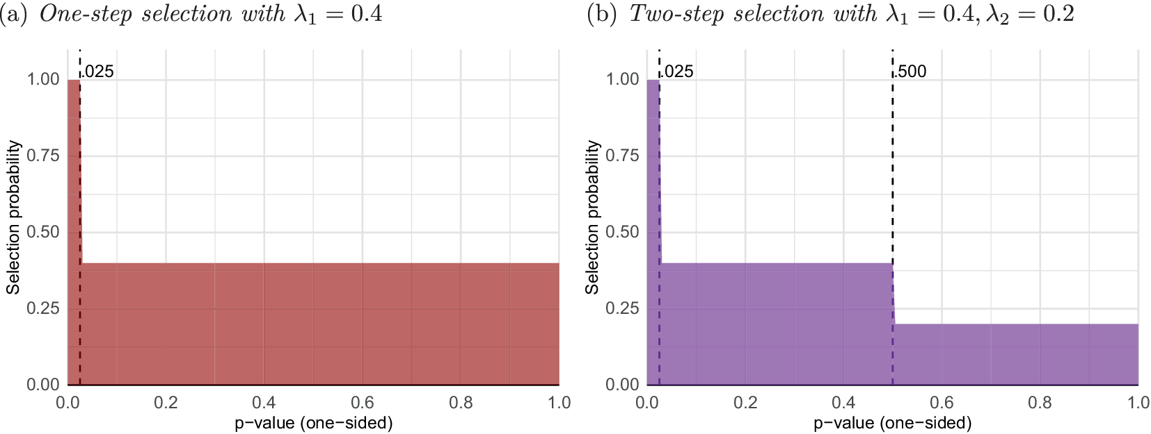
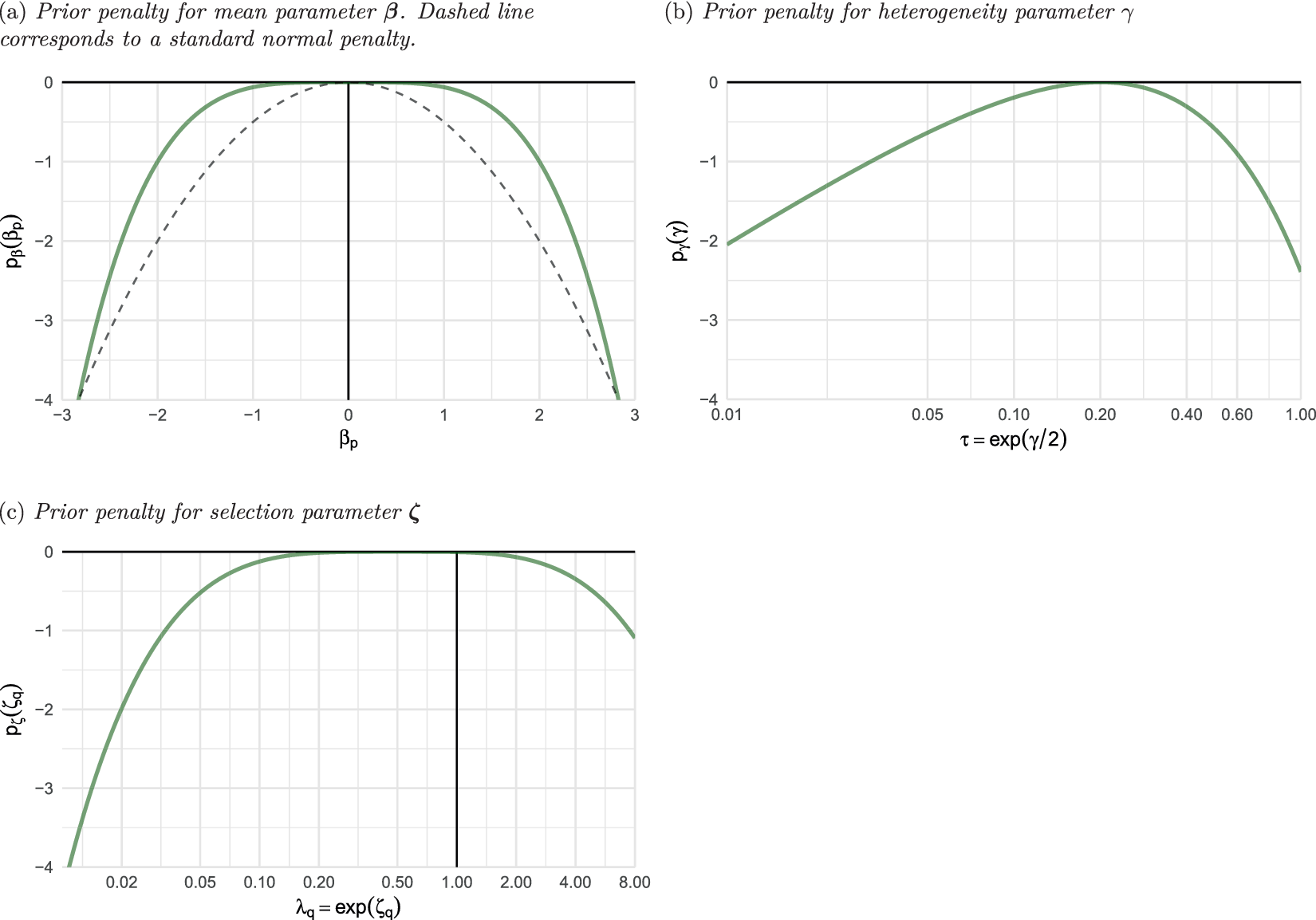
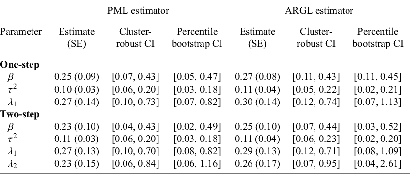
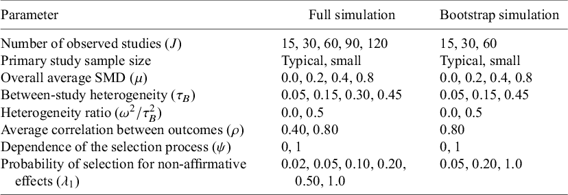


 Open access

