1 Introduction
Particle trajectories beneath a nonlinear periodic surface wave riding on a current represent a problem of great interest in both its environmental applications as well as in the mathematical theory of water waves. Related research on this theme goes back many years, such as, for example, the studies by Longuett-Higgins (Reference Longuett-Higgins1979) and Simmen & Saffman (Reference Simmen and Saffman1985), among others. A variety of theoretical and experimental (more recent) articles can be found in the special issue edited by Constantin (Reference Constantin2012) as well as in the articles by Constantin & Strauss (Reference Constantin and Strauss2004, Reference Constantin and Strauss2007, Reference Constantin and Strauss2011), Constantin (Reference Constantin2006), Ehrnström & Villari (Reference Ehrnström and Villari2008), Constantin & Varvaruca (Reference Constantin and Varvaruca2011) and Ehrnström, Escher & Villari (Reference Ehrnström, Escher and Villari2012) and their respective references.
It is known that for irrotational surface waves, particle trajectories follow loops with a mean Stokes drift in the wave propagation direction. Therefore, in the presence of a uniform counter-current, it is always possible to find closed orbits (Constantin & Strauss Reference Constantin and Strauss2010). Nachbin & Ribeiro Jr (Reference Nachbin and Ribeiro2014) observed this fact numerically with an accurate boundary integral method. A common model for waves in rotational flow is the case of constant vorticity. In this case, it is known that the travelling wave profiles remain symmetric (Toland Reference Toland2000; Constantin & Escher Reference Constantin and Escher2004a ), the streamlines are analytic (Lewy Reference Lewy1952) and the Stokes conjecture (Amick, Fraenkel & Toland Reference Amick, Fraenkel and Toland1982; Plotnikov Reference Plotnikov2002) is still valid (Constantin & Escher Reference Constantin and Escher2004b , Reference Constantin and Escher2011; Constantin, Ehrnström & Wahlén Reference Constantin, Ehrnström and Wahlén2007; Hur Reference Hur2007; Varvaruca Reference Varvaruca2009). The existence of periodic travelling wave solutions of large amplitude was proven in Constantin, Strauss & Varvaruca (Reference Constantin, Strauss and Varvaruca2014). The existence of exotic multi-valued profiles has been reported by Teles da Silva & Peregrine (Reference Teles da Silva and Peregrine1988) and further studied in Vanden-Broeck (Reference Vanden-Broeck1994, Reference Vanden-Broeck1996) and Choi (Reference Choi2009). However, the flow structure beneath a nonlinear rotational wave is relatively unexplored, and both numerical and theoretical results are quite scarce apart from some particle trajectory results for small-amplitude waves in Constantin & Villari (Reference Constantin and Villari2008), Ehrnström & Villari (Reference Ehrnström and Villari2008) and Wahlén (Reference Wahlén2009).
Important peculiarities of rotational waves are the existence of stagnation points (in the frame moving with the wave), pressure anomalies and critical layers in certain parameter regimes. We define a pressure anomaly when the maxima and minima of pressure occur in locations other than below the crest and trough respectively.
Early work by Teles da Silva & Peregrine (Reference Teles da Silva and Peregrine1988) inferred the presence of one stagnation point in the fluid through the streamline pattern. Pressure anomalies were also briefly reported. Choi (Reference Choi2003) and Ko & Strauss (Reference Ko and Strauss2008b
) also displayed the existence of one stagnation point through the streamline pattern, with the former considering only long waves. Very recently, Vasan & Oliveras (Reference Vasan and Oliveras2014) computed the streamlines and pressure level curves with a non-local formulation and provided evidence of the pressure anomaly mentioned in Teles da Silva & Peregrine (Reference Teles da Silva and Peregrine1988). They also inferred the existence of one stagnation point from the streamlines. In this paper, we present a more complete numerical study of the constant-vorticity flow due to a periodic gravity surface wave. We identify parameter regimes in which the flow has one, two or three stagnation points in a frame moving at the wave speed. The precise location of these critical points is important both in identifying cases in which there is a critical layer, namely a closed flow region with its corresponding separatrix (a ‘cat’s eye’ pattern), as well as in studying the bifurcation behaviour in terms of the parameter
 $\unicode[STIX]{x1D6FE}$
, the (constant) vorticity strength, and the wave-steepness parameter
 $\unicode[STIX]{x1D700}$
. The closed flow region, which is transported with the wave, is relevant to applications in tracer dispersal. We show, for example, that the three critical points (two saddles and a centre) that define a cat’s eye collide at the bottom and leave the flow domain as
 $\unicode[STIX]{x1D6FE}$
decreases. For a fixed vorticity
 $\unicode[STIX]{x1D6FE}$
, decreasing the steepness also leads to the collision of the stagnation points and a vanishing critical layer.
For irrotational waves, it is well known that the point of maximum pressure is at the bottom, directly below the wave crest (a proof is given in Constantin & Strauss Reference Constantin and Strauss2010). However, in the presence of large vorticity, a pressure anomaly arises (Teles da Silva & Peregrine Reference Teles da Silva and Peregrine1988; Ali & Kalish Reference Ali and Kalish2013; Vasan & Oliveras Reference Vasan and Oliveras2014). From our solutions, we identify two pressure anomalies: a minimum point of pressure within the bulk of the fluid and two points of maximum pressure away from the point below the crest and sometimes above the bottom. The points of anomalous pressure are associated with the hydrofoil-like effect of the critical layer, while the pressure maxima are associated with the two saddle (stagnation) points. The current work also details features of the fluid particle trajectories. Particle trajectories have not been analysed in detail either in the frame of reference of the wave or in the laboratory frame. Tracing the streamlines in the wave frame does not provide information regarding, for example, the variable velocity of the particle along its orbit or whether orbits are closed in the laboratory frame. In summary, we perform a quantitative study of the flow structure beneath a wave in the presence of constant vorticity. All of our results are obtained by combining calculations in a conformally mapped domain (where the free surface is flattened) together with the physical domain, in both the moving and laboratory frames of reference. The numerical method is implemented using Matlab.
This article is organised as follows. In § 2, we describe the mathematical formulation and our numerical implementation. In § 3, results from the numerical simulations are discussed, presenting the aforementioned results. The appendix briefly revisits the wave profile dependence on the vorticity and wave steepness, as well as some exotic wave profiles.
2 Formulation
We shall solve the problem of constant-vorticity water waves by first reducing the problem to one of potential flow (see, for example, Teles da Silva & Peregrine Reference Teles da Silva and Peregrine1988) and then using a conformal map from the uniform strip onto the flow domain, such as given by Choi (Reference Choi2009) and Milewski, Vanden-Broeck & Wang (Reference Milewski, Vanden-Broeck and Wang2010). In the canonical (flat) domain, Laplace’s equation can be solved analytically and the stationary boundary conditions are satisfied using a spectral collocation method. Once we have the solution in the canonical domain, the harmonic conformal map yields the solution in the physical domain.
2.1 Governing equations for waves with constant vorticity
Let
 $\boldsymbol{U}=(u(x,y,t),v(x,y,t))$
denote the velocity field in a region bounded below by a horizontal bottom and above by the free surface
 $y=\unicode[STIX]{x1D702}(x,t)$
. The Euler equations for an ideal fluid are
 $$\begin{eqnarray}\left.\begin{array}{@{}c@{}}\displaystyle \frac{\unicode[STIX]{x2202}\boldsymbol{U}}{\unicode[STIX]{x2202}t}+(\boldsymbol{U}\boldsymbol{\cdot }\unicode[STIX]{x1D735})\boldsymbol{U}=-\frac{1}{\unicode[STIX]{x1D70C}}\unicode[STIX]{x1D735}p-g\,\boldsymbol{j},\quad \text{in}~-d<y<\unicode[STIX]{x1D702}(x,t),\\ \displaystyle \unicode[STIX]{x1D735}\boldsymbol{\cdot }\boldsymbol{U}=0,\quad \text{in}~-d<y<\unicode[STIX]{x1D702}(x,t),\end{array}\right\}\end{eqnarray}$$
where
 $p(x,y,t)$
is the pressure,
 $\unicode[STIX]{x1D70C}$
is the constant fluid density,
 $g$
is the acceleration due to gravity and
 $\boldsymbol{j}=(0,1)$
. We have the boundary conditions
 $$\begin{eqnarray}\displaystyle & v=\unicode[STIX]{x1D702}_{t}+u\unicode[STIX]{x1D702}_{x},\quad \text{at}~y=\unicode[STIX]{x1D702}(x,t), & \displaystyle\end{eqnarray}$$
 $$\begin{eqnarray}\displaystyle & p=p_{atm},\quad \text{at}~y=\unicode[STIX]{x1D702}(x,t), & \displaystyle\end{eqnarray}$$
 $$\begin{eqnarray}\displaystyle & v=0,\quad \text{at}~y=-d, & \displaystyle\end{eqnarray}$$
where
 $p_{atm}$
is the atmospheric pressure. The vorticity is denoted by
 $$\begin{eqnarray}\unicode[STIX]{x1D6E4}:=v_{x}-u_{y}.\end{eqnarray}$$
Taking
 $\unicode[STIX]{x1D702}\equiv 0$
and a constant vorticity
 $\unicode[STIX]{x1D6E4}=\unicode[STIX]{x1D6FE}$
,
 $$\begin{eqnarray}\boldsymbol{U}_{\mathbf{0}}=(-\unicode[STIX]{x1D6FE}(y+b),0),\quad \text{in}~-d<y<0,b\in \mathbb{R},\end{eqnarray}$$
is a solution of (2.1), satisfying (2.2)–(2.4). The background flow
 $\boldsymbol{U}_{\mathbf{0}}$
is a linear shear flow. Now, consider
 $$\begin{eqnarray}\boldsymbol{U}=\boldsymbol{U}_{\mathbf{0}}+\unicode[STIX]{x1D735}\unicode[STIX]{x1D719},\end{eqnarray}$$
where
 $\unicode[STIX]{x1D719}$
is the velocity potential of an irrotational perturbation of the shear flow. Since
 $\unicode[STIX]{x1D6E4}$
is constant,
 $\unicode[STIX]{x1D6E4}$
and
 $\boldsymbol{U}$
satisfy the vorticity equation
 $\unicode[STIX]{x1D6E4}_{t}+(\boldsymbol{U}\boldsymbol{\cdot }\unicode[STIX]{x1D735})\unicode[STIX]{x1D6E4}=0$
, and thus only the incompressibility condition
 $\unicode[STIX]{x1D735}\boldsymbol{\cdot }\boldsymbol{U}=\unicode[STIX]{x0394}\unicode[STIX]{x1D719}=0$
remains to be satisfied in the fluid.
Equations (2.1)–(2.4) can written in dimensionless form as
 $$\begin{eqnarray}\left.\begin{array}{@{}c@{}}\unicode[STIX]{x0394}\unicode[STIX]{x1D719}=0,\quad \text{in}~-1<y<\unicode[STIX]{x1D702}(x,t),\\ \unicode[STIX]{x1D702}_{t}+(\unicode[STIX]{x1D719}_{x}-\unicode[STIX]{x1D6FE}(\unicode[STIX]{x1D702}+b))\unicode[STIX]{x1D702}_{x}=\unicode[STIX]{x1D719}_{y},\quad \text{at}~y=\unicode[STIX]{x1D702}(x,t),\\ \unicode[STIX]{x1D719}_{t}+{\textstyle \frac{1}{2}}(\unicode[STIX]{x1D719}_{x}^{2}+\unicode[STIX]{x1D719}_{y}^{2})+\unicode[STIX]{x1D702}-\unicode[STIX]{x1D6FE}(\unicode[STIX]{x1D702}+b)\unicode[STIX]{x1D719}_{x}+\unicode[STIX]{x1D6FE}\unicode[STIX]{x1D713}=B(t),\quad \text{at}~y=\unicode[STIX]{x1D702}(x,t),\\ \unicode[STIX]{x1D719}_{y}=0,\quad \text{at}~y=-1,\end{array}\right\}\end{eqnarray}$$
with the pressure in the fluid body given by
 $$\begin{eqnarray}p=-(\unicode[STIX]{x1D719}_{t}+{\textstyle \frac{1}{2}}(\unicode[STIX]{x1D719}_{x}^{2}+\unicode[STIX]{x1D719}_{y}^{2})+y-\unicode[STIX]{x1D6FE}(y+b)\unicode[STIX]{x1D719}_{x}+\unicode[STIX]{x1D6FE}\unicode[STIX]{x1D713}-B(t)).\end{eqnarray}$$
Here,
 $\unicode[STIX]{x1D713}$
is the streamfunction associated with
 $\unicode[STIX]{x1D719}$
(i.e. its harmonic conjugate) and
 $B(t)$
is the Bernoulli constant.
The equations have been non-dimensionalised using
 $d$
and
 $\sqrt{d/g}$
(as the characteristic length and time) in order to obtain a problem with a channel of unit depth, and unit linear long-wave speed. The dimensional quantities are therefore
 $$\begin{eqnarray}\left.\begin{array}{@{}c@{}}\text{d}x,\quad \text{d}y,\quad \text{d}b,\quad \text{d}\unicode[STIX]{x1D702},\quad \unicode[STIX]{x1D6FE}/\sqrt{d/g},\\ \unicode[STIX]{x1D719}\quad d\sqrt{gd},\quad t\sqrt{d/g},\quad \unicode[STIX]{x1D713}d\sqrt{gd},\quad g\,\text{d}B.\end{array}\right\}\end{eqnarray}$$
The dimensional pressure is given by
 $p_{atm}+(\unicode[STIX]{x1D70C}gd)p$
.
We now consider the case in which all functions are taken to be periodic in
 $x$
with wavelength
 $\unicode[STIX]{x1D706}$
, and travelling with speed
 $c$
. Thus, they can be written in terms of
 $X=(x-ct)$
and
 $Y=y$
. Without loss of generality, we assume that the mean of
 $\unicode[STIX]{x1D702}(x,t)$
is zero. The function
 $\unicode[STIX]{x1D702}$
is taken to be even and
 $\unicode[STIX]{x1D719}$
to be odd with respect to
 $x=0$
where the wave crest is positioned. In the frame moving with the wave, (2.8) becomes
 $$\begin{eqnarray}\left.\begin{array}{@{}c@{}}\unicode[STIX]{x0394}\unicode[STIX]{x1D719}=0,\quad \text{in}~-1<Y<\unicode[STIX]{x1D702}(X),\\ -c\unicode[STIX]{x1D702}_{X}+(\unicode[STIX]{x1D719}_{X}-\unicode[STIX]{x1D6FE}(\unicode[STIX]{x1D702}+b))\unicode[STIX]{x1D702}_{X}=\unicode[STIX]{x1D719}_{Y},\quad \text{at}~Y=\unicode[STIX]{x1D702}(X),\\ -c\unicode[STIX]{x1D719}_{X}+{\textstyle \frac{1}{2}}(\unicode[STIX]{x1D719}_{X}^{2}+\unicode[STIX]{x1D719}_{Y}^{2})+\unicode[STIX]{x1D702}-\unicode[STIX]{x1D6FE}(\unicode[STIX]{x1D702}+b)\unicode[STIX]{x1D719}_{X}+\unicode[STIX]{x1D6FE}\unicode[STIX]{x1D713}=B,\quad \text{at}~Y=\unicode[STIX]{x1D702}(X),\\ \unicode[STIX]{x1D719}_{Y}=0,\quad \text{at}~Y=-1,\end{array}\right\}\end{eqnarray}$$
and
 $$\begin{eqnarray}p=-(-c\unicode[STIX]{x1D719}_{X}+{\textstyle \frac{1}{2}}(\unicode[STIX]{x1D719}_{X}^{2}+\unicode[STIX]{x1D719}_{Y}^{2})+Y-\unicode[STIX]{x1D6FE}(Y+b)\unicode[STIX]{x1D719}_{X}+\unicode[STIX]{x1D6FE}\unicode[STIX]{x1D713}-B).\end{eqnarray}$$
2.2 The conformal map
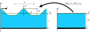
The conformal mapping from the canonical domain on the right onto the physical domain on the left.

The canonical strip is now conformally mapped onto the flow domain of the periodic steady wave. The coordinates in the canonical domain are
 $(\unicode[STIX]{x1D709},\unicode[STIX]{x1D701})$
and the conformal map is defined as
 $\widetilde{Z}(\unicode[STIX]{x1D709},\unicode[STIX]{x1D701})=\widetilde{X}(\unicode[STIX]{x1D709},\unicode[STIX]{x1D701})+\text{i}\widetilde{Y}(\unicode[STIX]{x1D709},\unicode[STIX]{x1D701})$
, as indicated in figure 1. The real and imaginary parts of the conformal map are conjugate harmonic functions. The wave elevation
 $\unicode[STIX]{x1D702}(X)$
provides the Dirichlet boundary data for
 $\widetilde{Y}$
. Thus, defining
 $\widetilde{\boldsymbol{Y}}(\unicode[STIX]{x1D709}):=\unicode[STIX]{x1D702}(\widetilde{X}(\unicode[STIX]{x1D709},0))$
, we solve the problem
 $$\begin{eqnarray}\left.\begin{array}{@{}c@{}}\unicode[STIX]{x0394}\widetilde{Y}=0,\quad \text{in}~-D<\unicode[STIX]{x1D701}<0,\\ \widetilde{Y}(\unicode[STIX]{x1D709},0)=\widetilde{\boldsymbol{Y}}(\unicode[STIX]{x1D709}),\\ \widetilde{Y}(\unicode[STIX]{x1D709},-D)=-1,\end{array}\right\}\end{eqnarray}$$
where the strip depth
 $D$
will be determined. The solution for
 $\widetilde{Y}$
is
 $$\begin{eqnarray}\widetilde{Y}(\unicode[STIX]{x1D709},\unicode[STIX]{x1D701})=\boldsymbol{F}^{-\mathbf{1}}\left[\frac{\sinh (k_{j}(\unicode[STIX]{x1D701}+D))}{\sinh (k_{j}D)}\boldsymbol{F}_{k}[\widetilde{\boldsymbol{Y}}]\right]+\frac{\unicode[STIX]{x1D701}}{D},\end{eqnarray}$$
where
 $k_{j}=(2\unicode[STIX]{x03C0}/L)j$
, for
 $j\in \mathbb{Z}$
, and
 $$\begin{eqnarray}\displaystyle & \displaystyle \boldsymbol{F}_{k}[g(\unicode[STIX]{x1D709})]=\widehat{g}(k_{j})={\displaystyle \frac{1}{L}}\int _{-L/2}^{L/2}g(\unicode[STIX]{x1D709})\text{e}^{-\text{i}k_{j}\unicode[STIX]{x1D709}}\,\text{d}\unicode[STIX]{x1D709}, & \displaystyle\end{eqnarray}$$
 $$\begin{eqnarray}\displaystyle & \displaystyle \boldsymbol{F}^{-1}[\widehat{g}(k_{j})](\unicode[STIX]{x1D709})=g(\unicode[STIX]{x1D709})=\mathop{\sum }_{j=-\infty }^{\infty }\widehat{g}(k_{j})\text{e}^{\text{i}k_{j}\unicode[STIX]{x1D709}}. & \displaystyle\end{eqnarray}$$
It should be noted that in (2.14) and elsewhere, unless indicated otherwise, the
 $j=0$
case is defined in the limit
 $k_{j}\rightarrow 0$
. Integrating the Cauchy–Riemann equation
 $\widetilde{X}_{\unicode[STIX]{x1D709}}=\widetilde{Y}_{\unicode[STIX]{x1D701}}$
, we obtain that
 $$\begin{eqnarray}\widetilde{X}(\unicode[STIX]{x1D709},\unicode[STIX]{x1D701})=(1+\langle \widetilde{\boldsymbol{Y}}\rangle )\frac{\unicode[STIX]{x1D709}}{D}-\boldsymbol{F}^{-\mathbf{1}}\left[\text{i}\frac{\cosh (k_{j}(\unicode[STIX]{x1D701}+D))}{\sinh (k_{j}D)}\boldsymbol{F}_{k}[\widetilde{\boldsymbol{Y}}]\right],\quad j\neq 0,\end{eqnarray}$$
where
 $$\begin{eqnarray}\langle \widetilde{\boldsymbol{Y}}\rangle ={\displaystyle \frac{1}{L}}\int _{-L/2}^{L/2}\widetilde{\boldsymbol{Y}}(\unicode[STIX]{x1D709})\,\text{d}\unicode[STIX]{x1D709}.\end{eqnarray}$$
Defining
 $\widetilde{\boldsymbol{X}}(\unicode[STIX]{x1D709}):=\widetilde{X}(\unicode[STIX]{x1D709},0)$
and taking the mean of
 $\widetilde{\boldsymbol{X}}_{\unicode[STIX]{x1D709}}(\unicode[STIX]{x1D709})$
yields
 $$\begin{eqnarray}\frac{1}{L}\int _{-L/2}^{L/2}\widetilde{\boldsymbol{X}}_{\unicode[STIX]{x1D709}}(\unicode[STIX]{x1D709})\,\text{d}\unicode[STIX]{x1D709}=\frac{1+\langle \widetilde{\boldsymbol{Y}}\rangle }{D}.\end{eqnarray}$$
On the other hand,
 $\int _{-L/2}^{L/2}\widetilde{\boldsymbol{X}}_{\unicode[STIX]{x1D709}}(\unicode[STIX]{x1D709})\,\text{d}\unicode[STIX]{x1D709}=\widetilde{\boldsymbol{X}}(L)-\widetilde{\boldsymbol{X}}(0)=\unicode[STIX]{x1D706}$
, and therefore
 $$\begin{eqnarray}\frac{\unicode[STIX]{x1D706}}{L}=\frac{1+\langle \widetilde{\boldsymbol{Y}}\rangle }{D}.\end{eqnarray}$$
Henceforth, we choose the wavelengths in both domains to be equal (
 $L=\unicode[STIX]{x1D706}$
), and therefore
 $$\begin{eqnarray}D=\langle \widetilde{\boldsymbol{Y}}\rangle +1.\end{eqnarray}$$
In the canonical domain, both
 $\widetilde{\unicode[STIX]{x1D719}}(\unicode[STIX]{x1D709},\unicode[STIX]{x1D701}):=\unicode[STIX]{x1D719}(\widetilde{X}(\unicode[STIX]{x1D709},\unicode[STIX]{x1D701}),\widetilde{Y}(\unicode[STIX]{x1D709},\unicode[STIX]{x1D701}))$
and its harmonic conjugate
 $\widetilde{\unicode[STIX]{x1D713}}(\unicode[STIX]{x1D709},\unicode[STIX]{x1D701}):=\unicode[STIX]{x1D713}(\widetilde{X}(\unicode[STIX]{x1D709},\unicode[STIX]{x1D701}),\widetilde{Y}(\unicode[STIX]{x1D709},\unicode[STIX]{x1D701}))$
satisfy the Laplace equation:
 $$\begin{eqnarray}\displaystyle & \displaystyle \left.\begin{array}{@{}c@{}}\unicode[STIX]{x0394}\widetilde{\unicode[STIX]{x1D719}}=0,\quad \text{in}~-D<\unicode[STIX]{x1D701}<0,\\ \widetilde{\unicode[STIX]{x1D719}}(\unicode[STIX]{x1D709},0)=\widetilde{\unicode[STIX]{x1D731}}(\unicode[STIX]{x1D709}),\\ \widetilde{\unicode[STIX]{x1D719}}_{\unicode[STIX]{x1D701}}(\unicode[STIX]{x1D709},-D)=0,\end{array}\right\} & \displaystyle\end{eqnarray}$$
 $$\begin{eqnarray}\displaystyle & \displaystyle \left.\begin{array}{@{}c@{}}\unicode[STIX]{x0394}\widetilde{\unicode[STIX]{x1D713}}=0,\quad \text{in}~-D<\unicode[STIX]{x1D701}<0,\\ \widetilde{\unicode[STIX]{x1D713}}(\unicode[STIX]{x1D709},0)=\widetilde{\unicode[STIX]{x1D733}}(\unicode[STIX]{x1D709}),\\ \widetilde{\unicode[STIX]{x1D713}}(\unicode[STIX]{x1D709},-D)=A,\end{array}\right\} & \displaystyle\end{eqnarray}$$
the solutions of which are given by
 $$\begin{eqnarray}\displaystyle & \displaystyle \widetilde{\unicode[STIX]{x1D719}}(\unicode[STIX]{x1D709},\unicode[STIX]{x1D701})=\boldsymbol{F}^{-\mathbf{1}}\left[\frac{\cosh (k_{j}(\unicode[STIX]{x1D701}+D))}{\cosh (k_{j}D)}\boldsymbol{F}_{k}[\widetilde{\unicode[STIX]{x1D731}}]\right], & \displaystyle\end{eqnarray}$$
 $$\begin{eqnarray}\displaystyle & \displaystyle \widetilde{\unicode[STIX]{x1D713}}(\unicode[STIX]{x1D709},\unicode[STIX]{x1D701})=\boldsymbol{F}^{-\mathbf{1}}\left[\frac{\sinh (k_{j}(\unicode[STIX]{x1D701}+D))}{\sinh (k_{j}D)}\boldsymbol{F}_{k}[\widetilde{\unicode[STIX]{x1D733}}]\right]-A{\displaystyle \frac{\unicode[STIX]{x1D701}}{D}}. & \displaystyle\end{eqnarray}$$
The arbitrary constant
 $A$
can be fixed by imposing that the mean horizontal velocity induced by the wave at the bottom is zero:
 $$\begin{eqnarray}\int _{-\unicode[STIX]{x1D706}/2}^{\unicode[STIX]{x1D706}/2}\unicode[STIX]{x1D713}_{Y}(X,-1)\,\text{d}X=0,\end{eqnarray}$$
fixing the laboratory frame of reference. Making the change of variables
 $X=\widetilde{X}(\unicode[STIX]{x1D709},-D)$
, we have that
 $$\begin{eqnarray}\int _{-\unicode[STIX]{x1D706}/2}^{\unicode[STIX]{x1D706}/2}\unicode[STIX]{x1D713}_{Y}(X,-1)\,\text{d}X=\int _{-L/2}^{L/2}\unicode[STIX]{x1D713}_{Y}(\widetilde{X}(\unicode[STIX]{x1D709},-D),-1)\widetilde{X}_{\unicode[STIX]{x1D709}}(\unicode[STIX]{x1D709},-D)\,\text{d}\unicode[STIX]{x1D709}.\end{eqnarray}$$
It is easy to show (as detailed in (2.33) and (2.34)) that
 $$\begin{eqnarray}\unicode[STIX]{x1D713}_{Y}={\displaystyle \frac{1}{|\text{J}|}}(\widetilde{\unicode[STIX]{x1D713}}_{\unicode[STIX]{x1D709}}\widetilde{X}_{\unicode[STIX]{x1D701}}+\widetilde{\unicode[STIX]{x1D713}}_{\unicode[STIX]{x1D701}}\widetilde{X}_{\unicode[STIX]{x1D709}}),\end{eqnarray}$$
where
 $|\text{J}|(\unicode[STIX]{x1D709},\unicode[STIX]{x1D701}):=\widetilde{X}_{\unicode[STIX]{x1D709}}^{2}+\widetilde{Y}_{\unicode[STIX]{x1D709}}^{2}$
. Restricted to the bottom, this results in
 $$\begin{eqnarray}\unicode[STIX]{x1D713}_{Y}(\widetilde{X}(\unicode[STIX]{x1D709},-D),-1)=\frac{\widetilde{\unicode[STIX]{x1D713}}_{\unicode[STIX]{x1D701}}(\unicode[STIX]{x1D709},-D)}{\widetilde{X}_{\unicode[STIX]{x1D709}}(\unicode[STIX]{x1D709},-D)},\end{eqnarray}$$
and therefore
 $$\begin{eqnarray}\int _{-\unicode[STIX]{x1D706}/2}^{\unicode[STIX]{x1D706}/2}\unicode[STIX]{x1D713}_{Y}(X,-1)\,\text{d}X=\int _{-L/2}^{L/2}\widetilde{\unicode[STIX]{x1D713}}_{\unicode[STIX]{x1D701}}(\unicode[STIX]{x1D709},-D)\,\text{d}\unicode[STIX]{x1D709}=0.\end{eqnarray}$$
Imposing
 $\langle \widetilde{\unicode[STIX]{x1D713}}_{\unicode[STIX]{x1D701}}(\unicode[STIX]{x1D709},-D)\rangle =0$
in (2.25), and taking the limit
 $k_{j}\rightarrow 0$
, yields
 $A=\langle \widetilde{\unicode[STIX]{x1D733}}\rangle$
.
Finally, we add that, using the Cauchy–Riemann equations
 $\widetilde{\unicode[STIX]{x1D719}}_{\unicode[STIX]{x1D709}}=\widetilde{\unicode[STIX]{x1D713}}_{\unicode[STIX]{x1D701}}$
and restricting ourselves to the free surface, it follows that
 $\text{i}k_{j}\boldsymbol{F}_{k}[\widetilde{\unicode[STIX]{x1D731}}]=k_{j}\coth (k_{j}D)\boldsymbol{F}_{k}[\widetilde{\unicode[STIX]{x1D733}}]$
and therefore
 $$\begin{eqnarray}\widetilde{\unicode[STIX]{x1D731}}=-{\mathcal{C}}[\widetilde{\unicode[STIX]{x1D733}}],\end{eqnarray}$$
with
 ${\mathcal{C}}[\cdot ]:=\boldsymbol{F}^{-\mathbf{1}}[\text{i}\coth (k_{j}D)]\boldsymbol{F}_{k}[\cdot ]$
. Similarly,
 $$\begin{eqnarray}\widetilde{\boldsymbol{X}}_{\unicode[STIX]{x1D709}}=1-{\mathcal{C}}[\widetilde{\boldsymbol{Y}}_{\unicode[STIX]{x1D709}}].\end{eqnarray}$$
2.3 The wave elevation equation
We now proceed to translate from the boundary conditions at the free surface to ones in the canonical domain. Since
 $\widetilde{\unicode[STIX]{x1D719}}(\unicode[STIX]{x1D709},\unicode[STIX]{x1D701}):=\unicode[STIX]{x1D719}(\widetilde{X}(\unicode[STIX]{x1D709},\unicode[STIX]{x1D701}),\widetilde{Y}(\unicode[STIX]{x1D709},\unicode[STIX]{x1D701}))$
, the derivatives of
 $\widetilde{\unicode[STIX]{x1D719}}$
are
 $$\begin{eqnarray}\left.\begin{array}{@{}c@{}}\widetilde{\unicode[STIX]{x1D719}}_{\unicode[STIX]{x1D709}}=\unicode[STIX]{x1D719}_{X}\widetilde{X}_{\unicode[STIX]{x1D709}}+\unicode[STIX]{x1D719}_{Y}\widetilde{Y}_{\unicode[STIX]{x1D709}},\\ \widetilde{\unicode[STIX]{x1D719}}_{\unicode[STIX]{x1D701}}=\unicode[STIX]{x1D719}_{X}\widetilde{X}_{\unicode[STIX]{x1D701}}+\unicode[STIX]{x1D719}_{Y}\widetilde{Y}_{\unicode[STIX]{x1D701}},\end{array}\right\}\end{eqnarray}$$
from which it follows that
 $$\begin{eqnarray}\left.\begin{array}{@{}c@{}}\displaystyle \unicode[STIX]{x1D719}_{X}={\displaystyle \frac{1}{|\text{J}|}}(\widetilde{\unicode[STIX]{x1D719}}_{\unicode[STIX]{x1D709}}\widetilde{Y}_{\unicode[STIX]{x1D701}}-\widetilde{\unicode[STIX]{x1D719}}_{\unicode[STIX]{x1D701}}\widetilde{Y}_{\unicode[STIX]{x1D709}}),\\ \displaystyle \unicode[STIX]{x1D719}_{Y}={\displaystyle \frac{1}{|\text{J}|}}(-\widetilde{\unicode[STIX]{x1D719}}_{\unicode[STIX]{x1D709}}\widetilde{X}_{\unicode[STIX]{x1D701}}+\widetilde{\unicode[STIX]{x1D719}}_{\unicode[STIX]{x1D701}}\widetilde{X}_{\unicode[STIX]{x1D709}}),\end{array}\right\}\end{eqnarray}$$
where
 $|\text{J}|(\unicode[STIX]{x1D709},\unicode[STIX]{x1D701}):=\widetilde{X}_{\unicode[STIX]{x1D709}}^{2}+\widetilde{Y}_{\unicode[STIX]{x1D709}}^{2}$
is the Jacobian of the map.
It should be noted that
 $$\begin{eqnarray}\widetilde{\boldsymbol{Y}}(\unicode[STIX]{x1D709})=\unicode[STIX]{x1D702}(\widetilde{X}(\unicode[STIX]{x1D709},0))\Rightarrow \widetilde{\boldsymbol{Y}}_{\unicode[STIX]{x1D709}}=\unicode[STIX]{x1D702}_{X}\widetilde{\boldsymbol{X}}_{\unicode[STIX]{x1D709}}\Rightarrow \unicode[STIX]{x1D702}_{X}=\frac{\widetilde{\boldsymbol{Y}}_{\unicode[STIX]{x1D709}}}{\widetilde{\boldsymbol{X}}_{\unicode[STIX]{x1D709}}}.\end{eqnarray}$$
Substituting into the kinematic boundary condition (2.11) yields
 $$\begin{eqnarray}-c\widetilde{\boldsymbol{Y}}_{\unicode[STIX]{x1D709}}+(\unicode[STIX]{x1D719}_{X}-\unicode[STIX]{x1D6FE}(\widetilde{\boldsymbol{Y}}+b))\widetilde{\boldsymbol{Y}}_{\unicode[STIX]{x1D709}}=\unicode[STIX]{x1D719}_{Y}\widetilde{\boldsymbol{X}}_{\unicode[STIX]{x1D709}}.\end{eqnarray}$$
Since
 $$\begin{eqnarray}\widetilde{\unicode[STIX]{x1D713}}(\unicode[STIX]{x1D709},\unicode[STIX]{x1D701})=\unicode[STIX]{x1D713}(\widetilde{X}(\unicode[STIX]{x1D709},\unicode[STIX]{x1D701}),\widetilde{Y}(\unicode[STIX]{x1D709},\unicode[STIX]{x1D701}))\Rightarrow \widetilde{\unicode[STIX]{x1D713}}_{\unicode[STIX]{x1D709}}=\unicode[STIX]{x1D713}_{X}\widetilde{X}_{\unicode[STIX]{x1D709}}+\unicode[STIX]{x1D713}_{Y}\widetilde{Y}_{\unicode[STIX]{x1D709}},\end{eqnarray}$$
using the Cauchy–Riemann equations to eliminate
 $\unicode[STIX]{x1D719}$
for
 $\unicode[STIX]{x1D713}$
, we substitute into the boundary condition (2.36), resulting in
 $$\begin{eqnarray}\widetilde{\unicode[STIX]{x1D733}}_{\unicode[STIX]{x1D709}}=c\widetilde{\boldsymbol{Y}}_{\unicode[STIX]{x1D709}}+\unicode[STIX]{x1D6FE}(\widetilde{\boldsymbol{Y}}+b)\widetilde{\boldsymbol{Y}}_{\unicode[STIX]{x1D709}}.\end{eqnarray}$$
Integrating that equation, we obtain
 $$\begin{eqnarray}\widetilde{\unicode[STIX]{x1D733}}=c\widetilde{\boldsymbol{Y}}+\unicode[STIX]{x1D6FE}\widetilde{\boldsymbol{Y}}\left(\frac{\widetilde{\boldsymbol{Y}}}{2}+b\right).\end{eqnarray}$$
We now proceed to the dynamic boundary condition. Using the equations (2.34) and the Cauchy–Riemann equations for (
 $\widetilde{X}$
,
 $\widetilde{Y}$
) and (
 $\widetilde{\unicode[STIX]{x1D719}}$
,
 $\widetilde{\unicode[STIX]{x1D713}}$
), we obtain that at the free surface (
 $\unicode[STIX]{x1D701}=0$
),
 $$\begin{eqnarray}\left.\begin{array}{@{}c@{}}\displaystyle \unicode[STIX]{x1D719}_{X}={\displaystyle \frac{1}{|\text{J}|}}(\widetilde{\unicode[STIX]{x1D731}}_{\unicode[STIX]{x1D709}}\widetilde{\boldsymbol{X}}_{\unicode[STIX]{x1D709}}+\widetilde{\unicode[STIX]{x1D733}}_{\unicode[STIX]{x1D709}}\widetilde{\boldsymbol{Y}}_{\unicode[STIX]{x1D709}}),\\ \displaystyle \unicode[STIX]{x1D719}_{Y}={\displaystyle \frac{1}{|\text{J}|}}(\widetilde{\unicode[STIX]{x1D731}}_{\unicode[STIX]{x1D709}}\widetilde{\boldsymbol{Y}}_{\unicode[STIX]{x1D709}}-\widetilde{\unicode[STIX]{x1D733}}_{\unicode[STIX]{x1D709}}\widetilde{\boldsymbol{X}}_{\unicode[STIX]{x1D709}}).\end{array}\right\}\end{eqnarray}$$
Substituting these equations and (2.35) into the dynamical condition in (2.11), we obtain
 $$\begin{eqnarray}\displaystyle & \displaystyle -{\displaystyle \frac{c}{|\text{J}|}}(\widetilde{\unicode[STIX]{x1D731}}_{\unicode[STIX]{x1D709}}\widetilde{\boldsymbol{X}}_{\unicode[STIX]{x1D709}}+\widetilde{\unicode[STIX]{x1D733}}_{\unicode[STIX]{x1D709}}\widetilde{\boldsymbol{Y}}_{\unicode[STIX]{x1D709}})+\frac{1}{2|\text{J}|}(\widetilde{\unicode[STIX]{x1D731}}_{\unicode[STIX]{x1D709}}^{2}+\widetilde{\unicode[STIX]{x1D733}}_{\unicode[STIX]{x1D709}}^{2})+\widetilde{\boldsymbol{Y}}+\unicode[STIX]{x1D6FE}\widetilde{\unicode[STIX]{x1D733}}-\unicode[STIX]{x1D6FE}(\widetilde{\boldsymbol{Y}}+b){\displaystyle \frac{1}{|\text{J}|}}(\widetilde{\unicode[STIX]{x1D731}}_{\unicode[STIX]{x1D709}}\widetilde{\boldsymbol{X}}_{\unicode[STIX]{x1D709}}+\widetilde{\unicode[STIX]{x1D733}}_{\unicode[STIX]{x1D709}}\widetilde{\boldsymbol{Y}}_{\unicode[STIX]{x1D709}})=B. & \displaystyle \nonumber\\ \displaystyle & & \displaystyle\end{eqnarray}$$
Equations (2.38) and (2.41) represent the free-surface boundary conditions in the canonical domain. Using (2.31) and (2.32), we combine them into a single equation for the free-surface elevation
 $\widetilde{\boldsymbol{Y}}=\unicode[STIX]{x1D702}(\widetilde{X}(\unicode[STIX]{x1D709},0))$
:
 $$\begin{eqnarray}\displaystyle & & \displaystyle -\frac{c^{2}}{2}-\frac{c^{2}}{2|\text{J}|}+\widetilde{\boldsymbol{Y}}+\unicode[STIX]{x1D6FE}^{2}\frac{({\mathcal{C}}[(\widetilde{\boldsymbol{Y}}+b)\widetilde{\boldsymbol{Y}}_{\unicode[STIX]{x1D709}}])^{2}-((\widetilde{\boldsymbol{Y}}+b)\widetilde{\boldsymbol{Y}}_{\unicode[STIX]{x1D709}})^{2}}{2|\text{J}|}+\unicode[STIX]{x1D6FE}^{2}\widetilde{\boldsymbol{Y}}\left(\frac{\widetilde{\boldsymbol{Y}}}{2}+b\right)\nonumber\\ \displaystyle & & \displaystyle \quad +\,\frac{(c+\unicode[STIX]{x1D6FE}{\mathcal{C}}[(\widetilde{\boldsymbol{Y}}+b)\widetilde{\boldsymbol{Y}}_{\unicode[STIX]{x1D709}}])(c+\unicode[STIX]{x1D6FE}(\widetilde{\boldsymbol{Y}}+b)(1-{\mathcal{C}}[\widetilde{\boldsymbol{Y}}_{\unicode[STIX]{x1D709}}]))}{|\text{J}|}-\unicode[STIX]{x1D6FE}cb=B.\end{eqnarray}$$
Hence, as unknowns, we have
 $\widetilde{\boldsymbol{Y}}(\unicode[STIX]{x1D709})$
,
 $c$
,
 $B$
and
 $D$
, and therefore (2.42) must be supplemented by three conditions: we fix the wave height
 $H$
through
 $$\begin{eqnarray}\widetilde{\boldsymbol{Y}}(0)-\widetilde{\boldsymbol{Y}}(\unicode[STIX]{x1D706}/2)=H,\end{eqnarray}$$
and we impose a mean-zero wave profile in the physical space,
 $$\begin{eqnarray}\int _{-\unicode[STIX]{x1D706}/2}^{0}\widetilde{\boldsymbol{Y}}\widetilde{\boldsymbol{X}}_{\unicode[STIX]{x1D709}}\,\text{d}\unicode[STIX]{x1D709}=0,\end{eqnarray}$$
as well as the depth condition (2.21)
 $$\begin{eqnarray}D=\langle \widetilde{\boldsymbol{Y}}\rangle +1.\end{eqnarray}$$
Equations (2.42)–(2.45) are solved using Newton’s method, as detailed in § 3.1.
Once a solution
 $\widetilde{\boldsymbol{Y}}$
is found, we use (2.39) to find
 $\widetilde{\unicode[STIX]{x1D733}}$
. The underlying velocity potential
 $\widetilde{\unicode[STIX]{x1D731}}$
is readily available from its harmonic conjugate
 $\widetilde{\unicode[STIX]{x1D733}}$
through the expression (2.31). Using the conformal mapping defined by (2.14), (2.17) and the harmonic function given by (2.25), the information needed for particle dynamics is complete. Namely, given a wave profile, we are in a position to compute values of
 $\widetilde{X}(\unicode[STIX]{x1D709},\unicode[STIX]{x1D701}),\widetilde{Y}(\unicode[STIX]{x1D709},\unicode[STIX]{x1D701})$
and
 $\widetilde{\unicode[STIX]{x1D713}}(\unicode[STIX]{x1D709},\unicode[STIX]{x1D701})$
anywhere in our canonical domain. The pressure is also readily available through expression (2.12).
2.4 Flow structure beneath the wave
In this section, we show how to use the formulation above in order to compute streamlines and stagnation points in a frame moving with the wave, as well as pressure and particle paths in arbitrary frames of reference.
In a frame moving with the speed
 $U$
, a fluid particle has the trajectory
 $(X(t),Y(t))$
satisfying
 $$\begin{eqnarray}\left.\begin{array}{@{}c@{}}\displaystyle \frac{\text{d}X}{\text{d}t}=\unicode[STIX]{x1D719}_{X}(X,Y)-\unicode[STIX]{x1D6FE}(Y+b)-U,\\ \displaystyle \frac{\text{d}Y}{\text{d}t}=\unicode[STIX]{x1D719}_{Y}(X,Y).\end{array}\right\}\end{eqnarray}$$
In the canonical domain, the corresponding trajectory
 $(\unicode[STIX]{x1D709}(t),\unicode[STIX]{x1D701}(t))$
, such that
 $(X(t),Y(t))=(\widetilde{X}(\unicode[STIX]{x1D709}(t),\unicode[STIX]{x1D701}(t)),\widetilde{Y}(\unicode[STIX]{x1D709}(t),\unicode[STIX]{x1D701}(t)))$
, is obtained from
 $$\begin{eqnarray}\left.\begin{array}{@{}c@{}}\displaystyle \frac{\text{d}\unicode[STIX]{x1D709}}{\text{d}t}=\frac{1}{|\text{J}|}[\widetilde{\unicode[STIX]{x1D719}}_{\unicode[STIX]{x1D709}}+(-\unicode[STIX]{x1D6FE}(\widetilde{Y}+b)-U)\widetilde{Y}_{\unicode[STIX]{x1D701}}],\\ \displaystyle \frac{\text{d}\unicode[STIX]{x1D701}}{\text{d}t}=\frac{1}{|\text{J}|}[\widetilde{\unicode[STIX]{x1D719}}_{\unicode[STIX]{x1D701}}-(-\unicode[STIX]{x1D6FE}(\widetilde{Y}+b)-U)\widetilde{Y}_{\unicode[STIX]{x1D709}}].\end{array}\right\}\end{eqnarray}$$
Setting
 $U=c$
yields the paths in a frame moving with the wave.
The identification of stagnation points provides the structure of the phase portrait for particle trajectories beneath the travelling wave. In particular, for a periodic velocity field, at least two stagnation points are necessary for a closed recirculation zone to travel with the wave speed. The location of the stagnation points and their dependence on wave parameters for travelling nonlinear waves has been an issue of research interest (Ko & Strauss Reference Ko and Strauss2008a
,Reference Ko and Strauss
b
), which we shall address in detail. In our periodic symmetric wave configuration, we shall search for a stagnation point
 $(X_{s},Y_{s})$
restricted to a subset of the fluid domain. Since the wave crest is at
 $(0,\unicode[STIX]{x1D702}(0))$
, by symmetry and periodicity,
 $\unicode[STIX]{x1D719}_{Y}(X,Y)$
must vanish at
 $X=-\unicode[STIX]{x1D706}/2,0,\unicode[STIX]{x1D706}/2$
. In addition, the impermeable bottom implies
 $\unicode[STIX]{x1D719}_{Y}(X,-1)=0$
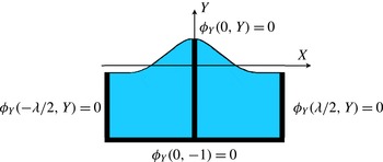
. Therefore, the vertical velocity is zero in the set depicted by a thick dark line in figure 2. In fact, under reasonable assumptions, stagnation points must lie in this region. Consider the vertical velocity field which is itself a harmonic function and which vanishes on this set. If the free boundary is monotonic on each side and has no stagnation points away from the wave crest, then the vertical velocity has a definite sign on the free surface on each side of the crest, and, by the maximum principle, can vanish only on the indicated set.
Locations for a vanishing vertical speed.

The search for stagnation points thus reduces to finding the zeros of
 $$\begin{eqnarray}U(X,Y):=\unicode[STIX]{x1D719}_{X}(X,Y)-\unicode[STIX]{x1D6FE}(Y+b)-c\end{eqnarray}$$
in the set shown in figure 2. With the present formulation, these zeros are found with great precision whatever the number of stagnation points. Since the horizontal velocity is symmetric with respect to
 $X=0$
, our search can be restricted to the right half of figure 2, namely within the viable set
 $V$
:
 $$\begin{eqnarray}V=\{(0,Y):Y\in [-1,\unicode[STIX]{x1D702}(0)]\}\cup \{(\unicode[STIX]{x1D706}/2,Y):Y\in [-1,\unicode[STIX]{x1D702}(\unicode[STIX]{x1D706}/2)]\}\cup \{(X,-1):X\in [0,\unicode[STIX]{x1D706}/2]\}.\end{eqnarray}$$
The pre-image of this set under the conformal mapping
 $(\widetilde{X}(\unicode[STIX]{x1D709},\unicode[STIX]{x1D701}),\widetilde{Y}(\unicode[STIX]{x1D709},\unicode[STIX]{x1D701}))$
is
 $$\begin{eqnarray}\widetilde{V}=\{(0,\unicode[STIX]{x1D701}):\unicode[STIX]{x1D701}\in [-D,0]\}\cup \{(\unicode[STIX]{x1D706}/2,\unicode[STIX]{x1D701}):\unicode[STIX]{x1D701}\in [-D,0]\}\cup \{(\unicode[STIX]{x1D709},-D):\unicode[STIX]{x1D709}\in [0,\unicode[STIX]{x1D706}/2]\}.\end{eqnarray}$$
Stagnation points are first found in the canonical domain using (2.24) and (2.34), and then mapped to the physical domain through (2.14) and (2.17).
In order to find the streamlines, the shear flow is added to
 $\widetilde{\unicode[STIX]{x1D713}}$
(the harmonic conjugate of
 $\unicode[STIX]{x1D719}$
), yielding the streamfunction
 $\unicode[STIX]{x1D713}_{T}$
:
 $$\begin{eqnarray}\unicode[STIX]{x1D713}_{T}:=\unicode[STIX]{x1D713}(\widetilde{X}(\unicode[STIX]{x1D709},\unicode[STIX]{x1D701}),\widetilde{Y}(\unicode[STIX]{x1D709},\unicode[STIX]{x1D701}))-\unicode[STIX]{x1D6FE}\widetilde{Y}(\unicode[STIX]{x1D709},\unicode[STIX]{x1D701})({\textstyle \frac{1}{2}}\widetilde{Y}(\unicode[STIX]{x1D709},\unicode[STIX]{x1D701})+b)-c\widetilde{Y}(\unicode[STIX]{x1D709},\unicode[STIX]{x1D701}).\end{eqnarray}$$
The streamfunction is evaluated on a uniform grid in the canonical plane. These values are assigned to the image grid in the physical domain and used to draw level curves of
 $\unicode[STIX]{x1D713}_{T}(X,Y)$
. A similar procedure is used for the pressure. From Bernoulli’s equation (2.12), we compute
 $$\begin{eqnarray}p=B+c\unicode[STIX]{x1D719}_{X}-{\textstyle \frac{1}{2}}(\unicode[STIX]{x1D719}_{X}^{2}+\unicode[STIX]{x1D719}_{Y}^{2})-Y+\unicode[STIX]{x1D6FE}(Y+b)\unicode[STIX]{x1D719}_{X}-\unicode[STIX]{x1D6FE}\unicode[STIX]{x1D713}\end{eqnarray}$$
on a uniform grid in the canonical domain, which is mapped to the physical domain having the corresponding pressure values assigned to its nodes.
3 Numerical simulations
In this section, we briefly present the method, followed by results of numerical simulations for a range of amplitude, wavelength and vorticity parameters. In the remainder of the paper, the depth is fixed and wavelengths are chosen such as to span both shallow water and deep water regimes. The amplitude parameter
 $H$
is defined as
 $$\begin{eqnarray}H=\unicode[STIX]{x1D702}(0)-\unicode[STIX]{x1D702}(-\unicode[STIX]{x1D706}/2)=\widetilde{\boldsymbol{Y}}(0)-\widetilde{\boldsymbol{Y}}(-\unicode[STIX]{x1D706}/2).\end{eqnarray}$$
We shall focus on two cases, always fixing the depth to 1. In the intermediate-depth case, we fix
 $\unicode[STIX]{x1D706}=2\unicode[STIX]{x03C0}$
and either vary
 $\unicode[STIX]{x1D6FE}$
or the steepness parameter
 $\unicode[STIX]{x1D700}=H/\unicode[STIX]{x1D706}$
. In the second case, we study depth effects by fixing the wave height
 $H$
and changing
 $\unicode[STIX]{x1D706}$
.
The effect of vorticity on the travelling wave profile has been studied by Teles da Silva & Peregrine (Reference Teles da Silva and Peregrine1988), Vanden-Broeck (Reference Vanden-Broeck1994, Reference Vanden-Broeck1996), Ko & Strauss (Reference Ko and Strauss2008b
) and Vasan & Oliveras (Reference Vasan and Oliveras2014). In summary, their results for the branch of rotational travelling waves with
 $c>0$
include the following.
-
(i) Waves in the presence of negative vorticity have narrower crests. Positive vorticity waves have profiles that become rounder with increasing amplitude and can form an exotic overhanging free surface over a thin layer of fluid. Within these disk-shaped regions, the fluid is in quasi-rigid-body rotation.
-
(ii) Larger waves can be constructed in the presence of positive vorticity. Negative vorticity significantly reduces the maximum wave amplitude. The limiting wave has either a Stokes-like
 $120^{\circ }$
crest angle or a disc shape. The precise conditions for one or the other limiting form are not known.

In appendix A, we detail how our method captured the properties above.
3.1 Computing the waves
Recall that the full solution in the canonical domain can be computed in a straightforward fashion as soon as the
 $\unicode[STIX]{x1D706}$
-periodic wave elevation
 $\widetilde{\boldsymbol{Y}}$
has been found, by solving (2.42)–(2.45). Take an equally spaced set of grid points in
 $\unicode[STIX]{x1D709}$
at
 $\unicode[STIX]{x1D701}=0$
in the canonical domain:
 $$\begin{eqnarray}\unicode[STIX]{x1D709}_{j}=-\frac{\unicode[STIX]{x1D706}}{2}+(j-1)\unicode[STIX]{x0394}\unicode[STIX]{x1D709},\quad j=1,\ldots ,N,\quad \text{where}~\unicode[STIX]{x0394}\unicode[STIX]{x1D709}=\unicode[STIX]{x1D706}/N.\end{eqnarray}$$
With
 $N$
even, let
 $\widetilde{\boldsymbol{Y}}_{j}:=\widetilde{\boldsymbol{Y}}(\unicode[STIX]{x1D709}_{j})$
and
 $\widetilde{\boldsymbol{X}}_{j}:=\widetilde{\boldsymbol{X}}(\unicode[STIX]{x1D709}_{j})$
, and impose even symmetry about
 $\unicode[STIX]{x1D709}=0$
by taking
 $\widetilde{\boldsymbol{Y}}_{j}:=\widetilde{\boldsymbol{Y}}_{N-j+2}$
,
 $j=N/2+2,\ldots ,N$
.
Substituting these into a discretised version of (2.42) gives rise to a set of
 $N/2+1$
equations for
 $N/2+4$
unknowns
 $(\widetilde{\boldsymbol{Y}}_{1},\ldots ,\widetilde{\boldsymbol{Y}}_{N/2+1},c,B,D)$
. The discretisation we have chosen replaces all derivatives and non-local linear operators in (2.42) and (2.32) by their discretised Fourier symbol. Thus, their action is computed with spectral accuracy in Fourier space and all nonlinearities are computed in real space at the grid points. The
 $N/2+1$
equations are obtained by evaluating (2.42) at grid points
 $\widetilde{\boldsymbol{X}}_{j}$
,
 $j=1,\ldots ,N/2+1$
. These can be expressed as
 $$\begin{eqnarray}G_{j}(\widetilde{\boldsymbol{Y}}_{1},\ldots ,\widetilde{\boldsymbol{Y}}_{N/2+1},c,B,D)=0,\quad j=1,\ldots ,N/2+1.\end{eqnarray}$$
The system is closed with the discretisation of the additional equations (2.43)–(2.45):
 $$\begin{eqnarray}\left.\begin{array}{@{}c@{}}\displaystyle G_{N/2+2}(\widetilde{\boldsymbol{Y}}_{1},\ldots ,\widetilde{\boldsymbol{Y}}_{N/2+1},c,B,D):=\widetilde{\boldsymbol{Y}}_{N/2+1}-\widetilde{\boldsymbol{Y}}_{1}-H=0,\\ \displaystyle G_{N/2+3}(\widetilde{\boldsymbol{Y}}_{1},\ldots ,\widetilde{\boldsymbol{Y}}_{N/2+1},c,B,D):=\frac{\widetilde{\boldsymbol{Y}}_{1}\widetilde{\boldsymbol{X}}_{\unicode[STIX]{x1D709}1}+\widetilde{\boldsymbol{Y}}_{N/2+1}\widetilde{\boldsymbol{X}}_{\unicode[STIX]{x1D709}(N/2+1)}}{2}\unicode[STIX]{x0394}\unicode[STIX]{x1D709}+\unicode[STIX]{x0394}\unicode[STIX]{x1D709}\mathop{\sum }_{j=2}^{N/2}\widetilde{\boldsymbol{Y}}_{j}\widetilde{\boldsymbol{X}}_{\unicode[STIX]{x1D709}j}=0,\\ \displaystyle G_{N/2+4}(\widetilde{\boldsymbol{Y}}_{1},\ldots ,\widetilde{\boldsymbol{Y}}_{N/2+1},c,B,D):=\frac{2}{N}\left(\frac{\widetilde{\boldsymbol{Y}}_{1}+\widetilde{\boldsymbol{Y}}_{N/2+1}}{2}+\mathop{\sum }_{j=2}^{N/2}\widetilde{\boldsymbol{Y}}_{j}\right)+1-D=0.\end{array}\right\}\end{eqnarray}$$
The system is solved by Newton’s method, with linear irrotational waves as initial guess:
 $$\begin{eqnarray}\unicode[STIX]{x1D6FE}=0,\quad \widetilde{\boldsymbol{Y}}(X)=(H/2)\cos (kX),\quad c=\sqrt{\frac{\tanh (k)}{k}},\quad B=0,\quad D=1,\end{eqnarray}$$
where
 $H$
is small. The solution can then be continued in the parameters (
 $H,\unicode[STIX]{x1D6FE},c$
) by using the prior converged solution as the initial guess to a new solution. The Jacobian of the system for the Newton iteration is found by finite variations in the unknowns. The stopping criterion is given by
 $$\begin{eqnarray}{\displaystyle \frac{\displaystyle \mathop{\sum }_{j=1}^{N/2+4}|G_{j}|}{N/2+4}}<10^{-10}.\end{eqnarray}$$
Due to Galilean invariance, the parameter
 $b$
affects neither the shape of the wave nor the streamlines in the frame of reference travelling with the wave. For simplicity, we always choose
 $b=0.5$
, corresponding to zero velocity at mid-depth for linear waves.
Particle trajectories are found by integrating in time the ordinary differential equations (2.47) in the canonical domain with a fourth-order Runge–Kutta method and mapping these trajectories on the moving frame
 $(X,Y)$
as described in § 2.4. Once we have computed
 $(X(t),Y(t))$
, the orbits in the laboratory frame of reference
 $(x,y)$
are obtained from
 $x(t)=X(t)+ct$
,
 $y(t)=Y(t)$
.
3.2 Streamlines and stagnation points
For surface waves in the absence of vorticity, it is known that there can be only one critical (stagnation) point, namely at the
 $120^{\circ }$
crest of the largest Stokes wave (Plotnikov Reference Plotnikov2002). For constant vorticity, various computations have provided evidence of either one or three stagnation points for certain values of
 $\unicode[STIX]{x1D6FE}$
(Teles da Silva & Peregrine Reference Teles da Silva and Peregrine1988; Ko & Strauss Reference Ko and Strauss2008b
; Vasan & Oliveras Reference Vasan and Oliveras2014). There is also an analysis by Constantin et al. (Reference Constantin, Strauss and Varvaruca2014) regarding the location of critical points under certain conditions. Here, we make a comprehensive study of the configurations and precise positions of stagnation points. We study their location dependence with respect to
 $\unicode[STIX]{x1D6FE}$
and wave amplitude. Having this in mind, we consider two types of parameter sweeps in system (2.46): (1) fixing a value of
 $\unicode[STIX]{x1D700}$
and varying
 $\unicode[STIX]{x1D6FE}$
; (2) fixing a value of
 $\unicode[STIX]{x1D6FE}$
and varying
 $\unicode[STIX]{x1D700}$
. The search for the stagnation point position and the construction of the system phase portrait are performed as described in § 2.4.
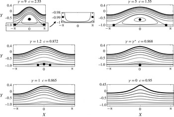
Phase portraits for waves with steepness
 $\unicode[STIX]{x1D700}=0.09$
for varying vorticity
 $\unicode[STIX]{x1D6FE}$
. The markers indicate the locations of the stagnation points (circles correspond to centres and squares to saddles).

We begin with a detailed study of an intermediate-depth regime where the wavelength is
 $2\unicode[STIX]{x03C0}$
(recall that the depth is always set to 1). In figure 3, a parameter sweep with
 $\unicode[STIX]{x1D700}=0.09$
is shown for values from
 $\unicode[STIX]{x1D6FE}=0$
up to the maximum vorticity value we can compute for this steepness. The stagnation points are shown with circles (centres) and squares (saddles). For large values of vorticity, there are two stagnation points inside the flow: a centre below the crest and a saddle below the trough, resulting in a cat’s eye region of closed streamlines (recirculation zone) centred below the crest. As
 $\unicode[STIX]{x1D6FE}$
decreases, the saddle point moves downward and reaches the lower boundary at
 $\unicode[STIX]{x1D6FE}\approx 6.8525$
, where the saddle splits into two. The recirculation zone is now attached to the lower boundary. As
 $\unicode[STIX]{x1D6FE}$
decreases further, this attached recirculation zone shrinks and disappears at
 $\unicode[STIX]{x1D6FE}^{\ast }\approx 1.0873$
when the three stagnation points coalesce at
 $x=0$
and disappear in a higher-order saddle–centre bifurcation. For smaller values of
 $\unicode[STIX]{x1D6FE}$
, the streamlines are qualitatively similar to Stokes waves. As expected, decreasing vorticity sharpens the crests.
We note that, as all of the bifurcations of the flow field occur at the lower boundary, they are simpler to understand if the flow is reflected symmetrically about this line. In this interpretation, the first bifurcation above is the result of the transcritical collision of two saddles, the one in the fluid and its image below the bottom boundary. After collision, they separate along the bottom boundary, creating the two stagnation points which are the leading and trailing edges of the recirculation zone. The second bifurcation corresponds to two saddles and two centres (one of which is below the bottom boundary) annihilating at the point
 $(0,-1)$
.
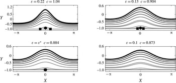
Phase portraits for waves with
 $\unicode[STIX]{x1D6FE}=1$
at different values of the wave steepness
 $\unicode[STIX]{x1D700}$
. The markers indicate the location of the stagnation points (circles correspond to centres and squares to saddles).

In figure 4, a parameter sweep with
 $\unicode[STIX]{x1D6FE}=1$
is shown for values of
 $\unicode[STIX]{x1D700}=0.1$
up to
 $\unicode[STIX]{x1D700}=0.22$
. In this sweep, the flow never exhibits the cat’s eye flow, as the recirculation zone is always attached to the bottom boundary at large amplitudes. As
 $\unicode[STIX]{x1D700}$
decreases, the same behaviour occurs as observed in the second bifurcation described in the paragraph above: the three stagnation points disappear at the bottom (for
 $\unicode[STIX]{x1D700}^{\ast }\approx 0.1113$
) under the crest, and the resulting flow resembles that of a small-amplitude periodic irrotational Stokes wave. In this regime, as the amplitude increases the waves become more peaked.
Parameter dependence of flow fields as the wave steepness
 $\unicode[STIX]{x1D700}$
and vorticity
 $\unicode[STIX]{x1D6FE}$
are varied while the depth and wavelength are held fixed at
 $1$
and
 $2\unicode[STIX]{x03C0}$
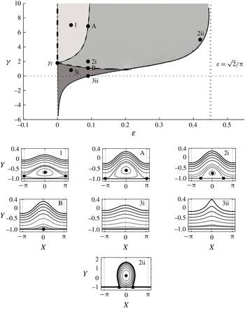
respectively. The dashed lines A and B correspond to points at which bifurcations occur, changing the number of stagnation points in the fluid domain. The vertical bold dash–dot line corresponds to a linearised flow with a stagnation point. The vertical dashed asymptote corresponds to the large-
 $\unicode[STIX]{x1D6FE}$
limit of rigid-body rotation and the solid curve to the largest waves we have computed at each value of vorticity. The three regions correspond to two, three or zero stagnation points within one period of the wave. Streamline profiles corresponding to the parameters indicated in the figure are also shown illustrating each case. The curve beyond point 2ii, as it asymptotes to the value
 $\unicode[STIX]{x1D700}=\sqrt{2}/\unicode[STIX]{x03C0}$
, has been schematically extended by the authors.

The full
 $(\unicode[STIX]{x1D700},\unicode[STIX]{x1D6FE})$
parameter space for
 $\unicode[STIX]{x1D706}=2\unicode[STIX]{x03C0}$
is shown in figure 5, together with typical flow patterns. The curve with vertical asymptotes at
 $\unicode[STIX]{x1D700}=0$
and
 $\unicode[STIX]{x1D700}=\sqrt{2}/\unicode[STIX]{x03C0}$
corresponds to the locus of the largest-amplitude waves that we could compute by our method. The asymptote at
 $\unicode[STIX]{x1D700}=\sqrt{2}/\unicode[STIX]{x03C0}$
corresponds to the limit in which the full fluid domain is in rigid-body rotation. The point
 $(0,\unicode[STIX]{x1D6FE}_{l}),\unicode[STIX]{x1D6FE}_{l}=\tanh (1)/(1-\tanh (1))$
is found by considering whether the linearised flow admits stagnation points on the lower boundary. As
 $\unicode[STIX]{x1D6FE}$
increases on points
 $(0,\unicode[STIX]{x1D6FE}),\unicode[STIX]{x1D6FE}>\unicode[STIX]{x1D6FE}_{l}$
, the stagnation point rises into the fluid. The dash–dot bold line in the figure indicates the range of
 $\unicode[STIX]{x1D6FE}$
such that the linearised flow has a stagnation point inside the fluid domain. The dashed lines correspond to bifurcation points at which the number of stagnation points in the domain changes. The bold dashed line B separates region 3 of ‘irrotational-like’ behaviour, with no stagnation points in the fluid, and region 2, with three stagnation points: two saddles at the lower boundary and a centre under the crest. On B, there is one stagnation point at the lower boundary under the crest. The thin dashed line A separates region 2 from region 1, where there are two stagnation points. This loss of a saddle point occurs when the two saddles at the lower boundary are exactly one wavelength apart and merge under the trough of the wave. Within region 1, this saddle moves inside the fluid, under the trough.
Phase portraits with
 $H=0.4$
,
 $\unicode[STIX]{x1D6FE}=10$
and varying the wavelength with
 $\unicode[STIX]{x1D706}=0.6$
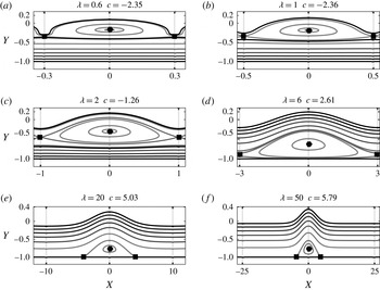
, 1, 2, 6, 20, 50. The black markers depict the stagnation points as before. The thick black curve is at
 $\unicode[STIX]{x1D713}(X,Y)=0$
. It should be noted that these solutions have different wavelengths from those in figure 5 and therefore correspond to different wavelength regimes: from short waves to long waves, from (a–f).

We now turn our attention to the effect of the wavelength, focusing on the most interesting case of large positive vorticity. We fix
 $\unicode[STIX]{x1D6FE}=10$
, set the depth to unity and fix the amplitude as
 $H=0.4$
as we vary the wavelength
 $\unicode[STIX]{x1D706}$
from the short-wave (deep water) regime (
 $\unicode[STIX]{x1D706}=0.6$
) to the long-wave (shallow water) regime (
 $\unicode[STIX]{x1D706}=50$
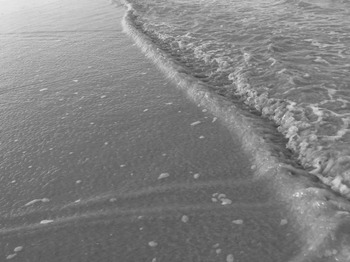
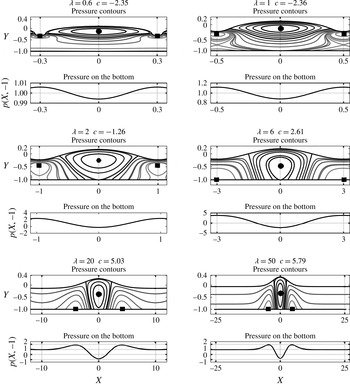
). This parameter choice allows us to keep the solutions strongly nonlinear throughout the range. The results are shown in figure 6. In deep water, the wave affects only an upper layer of depth approximately equal to the wavelength, with a large recirculation zone near the crest. As the depth decreases, this recirculation zone descends and there are counter-propagating currents above and below the cat’s eye. As the relative depth further decreases, the recirculation zone attaches to the bottom and forms a stationary fluid region at the bottom with a free-surface streaming flow above it. The free-surface profile here is similar to a ‘surface shear wave’ discussed in Peregrine (Reference Peregrine1974) which is often seen in backwash on a beach (see figure 7).
Nearly steady rounded wave profiles in the presence of a strongly shearing backwash flow. Photo by Roberto Ribeiro Jr.

3.3 Pressure
For irrotational flows, the following pressure properties are rigorously known (Constantin & Strauss Reference Constantin and Strauss2010, p. 539):
-
(i) the maximum pressure value is attained at the bottom, below the crest;
-
(ii) the minimum pressure value is attained at the free surface;
-
(iii) the pressure is strictly increasing with depth along a vertical line;
-
(iv) the pressure is strictly decreasing along horizontal lines starting below the crest and ending below the trough.
In the presence of constant vorticity, none of these facts hold in general. For example, recently Strauss & Wheeler (Reference Strauss and Wheeler2016, Proposition 16) proved that any wave that overturns has a pressure sink (minimum pressure) inside the fluid region, provided that it has no stagnation point on the free surface. By periodicity and symmetry about
 $x=0$
, the values of pressure below the crest or trough must be local extrema with respect to horizontal variations. Furthermore, the pressure at any saddle point on the bottom boundary must be a local maximum by Bernoulli’s theorem since the bottom is a streamline, and the pressure must also decrease along the other streamlines originating at that point and going upwards into the domain. This means that, referring to figure 5, we expect that for the pressure along the bottom, region 3 will behave like irrotational waves, while region 2 will have a local minimum under both crest and trough, and a maximum at the saddles. By a continuity argument, region 1 will have a maximum under the trough and a minimum under the crest.
Pressure beneath a periodic wave of steepness
 $\unicode[STIX]{x1D700}=0.09$
, as the background vorticity is varied. Black dots and squares represent the locations of global minima and maxima of pressure respectively. The thick black curve indicates the contour for
 $p(X,Y)=0$
. Also shown is the pressure along the bottom boundary.

Figure 8 displays the contours of the computed pressure field and the pressure on the bottom boundary for wave steepness
 $\unicode[STIX]{x1D700}=0.09$
and the various values of
 $\unicode[STIX]{x1D6FE}$
used in figure 3. In the figure, the thick black curves correspond to
 $p(X,Y)=0$
, the black dot indicates the point of global minimum pressure (when it is below atmospheric pressure) and the black square indicates the point of global maximum of pressure. As the vorticity increases, a below-atmospheric minimum pressure appears inside the fluid domain, whereas the maximum pressure has moved from below the crest to below the trough. In general, neither the pressure along a vertical line below the crest or trough, nor along a horizontal line from under the crest is monotonic. Some of these properties had been reported by Teles da Silva & Peregrine (Reference Teles da Silva and Peregrine1988) and Vasan & Oliveras (Reference Vasan and Oliveras2014).
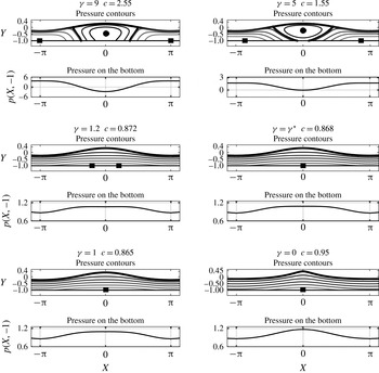
Pressure beneath a wave, in the different regimes shown in figure 6. In the pressure contour graphs, the black dots and squares represent the locations of minimum and maximum pressure respectively. The thick black curve denotes
 $p(X,Y)=0$
.

Figure 9 shows the effect of varying the depth (for the same cases as in figure 6). Except in very shallow water, the global minimum of pressure lies inside the recirculation zone, near the stagnation point under the crest, and the global maximum in pressure lies near the stagnation point under the trough. In shallow water, when the recirculation zone is attached to the bottom, the minimum in pressure moves upwards to a point above the crest of this recirculation zone.
3.3.1 Particle trajectories
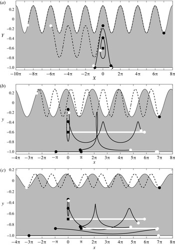
There are some results in the literature regarding particle trajectory patterns for water waves with vorticity in the presence of stagnation points. Wahlén (Reference Wahlén2009) obtained results based on a local bifurcation theory while Ehrnström & Villari (Reference Ehrnström and Villari2008) obtained results by linearising the governing equations about a shearing flow. Both analyses obtained information on the velocity field and subsequently the particle trajectories for arbitrarily small wave amplitudes. Here, through computational simulations, we show sample particle trajectory patterns in both the frame moving with the wave and a ‘laboratory’ frame. The definition of a laboratory frame is somewhat arbitrary. Here, we choose the frame in which the mean horizontal component of velocity is zero at the mid-depth (
 $Y=-1/2$
). It should be noted that since we have chosen
 $b=1/2$
for the vorticity component, it means that, in the limit of zero-amplitude waves, this choice of frame corresponds to a flow with no net mass flux on a vertical cut.
Particle trajectories, where a black dot indicates the initial position of a particle while a white dot is its final position after three wave periods have elapsed. The square markers depict the stagnation points. (a) Particle trajectories in the moving frame of the wave. The wave steepness is
 $\unicode[STIX]{x1D700}=0.09$
, the vorticity is
 $\unicode[STIX]{x1D6FE}=7$
and the velocity of the wave is
 $c=2.0416$
. (b) Particle trajectories for the same wave in the ‘laboratory’ frame. (c) The wave steepness is
 $\unicode[STIX]{x1D700}=0.04$
,
 $\unicode[STIX]{x1D6FE}=7$
and
 $c=1.9848$
. The saddle points are now further away from the bottom and clearly flow horizontally with the wave speed.

In figure 10, we display particle trajectories for a flow with two stagnation points and a recirculation zone nearly attached to the bottom in both the moving frame (a) as well as the laboratory frame (b). The trajectories are followed for three wave periods, and their start and end positions are indicated. In the moving wave frame with
 $c>0$
, it is expected that near the crest the particles move rapidly to the left, while in the recirculation zone they are trapped. In the laboratory frame, the (positive) vorticity is clearly visible, transporting particles near the bottom to the right and those near the top to the left. The recirculation zone manifests itself as a region of particles travelling, on average, with the speed of the wave. Figure 10(c) is a case for which the recirculation zone has moved upwards towards the mid-depth of the channel, and in this case the particle trajectories are shown in the laboratory frame only. We note that the particles in the trapped zone exhibit both strong transport with the wave and strong vertical oscillations, neither of which occurs in irrotational waves.
4 Conclusions
In this paper, we have focused on describing the properties of the flow under a steadily travelling periodic surface wave on a fluid of constant vorticity. The flow may be written as the superposition of a linear shear and a harmonic velocity potential. The problem was approached by conformally mapping a period of the wave to a rectangle where the velocity potential can be solved for easily, and a spectral numerical approach was used to solve the boundary conditions at the free surface. Once the solution is found, the explicit maps can be used to extract velocity field, streamfunction and pressure information in the physical domain.
Examination of the flow structure in the frame moving with the wave shows that the fluid can have one, two or three stagnation points. Flows may have a single stagnation point at the crest (like that of a Stokes wave) or at the bottom under the crest. In this latter case, increasing the vorticity results in a flow with three stagnation points (born out of a degenerate saddle–node bifurcation) and a recirculation zone attached to the bottom boundary. The flow may also have, above a certain value of vorticity and for amplitudes below a threshold, two stagnation points – a centre below the crest and a saddle below the trough – in a classic cat’s eye flow. At large amplitudes, exotic rounded waves approximate a rigid-body rotation flow. The pressure below the waves also exhibits unusual features, with maxima and minima at the bottom exchanged from the irrotational case.
Given the rich possibilities in the flow structure, particle trajectories can also be quite distinct from the irrotational case. Particles can undergo large vertical excursions and average horizontal transport at the wave speed. These effects could have environmental consequences, for example in the transport of pollutants or other material, wherever water waves and shear are present simultaneously.
Acknowledgements
We thank the anonymous referee for the simple argument in § 2.4 regarding the location of stagnation points. The work of P.A.M. was supported in part by a Royal Society Wolfson award and a CNPq-Science without Borders award no. 402178/2012-2. The work of A.N. was supported in part by CNPq under (PQ-1B) 301949/2007-7, FAPERJ Cientistas do Nosso Estado project no. 102.917/2011 and CAPES(ESN) no. 4156/13-7. The work of R.R.Jr was supported in part by CNPq-Science without Borders under (PDE) 200920/2014-6 and Petrobras through the program ANP/PETROBRAS PRH 32 projects no. 6000.0061847.10.4 and no. 6000.0069459.11.4. The authors A.N. and R.R.Jr are grateful to the University of Bath for extended visits to the Department of Mathematical Sciences and would like to thank Professor A. Constantin for useful conversations at King’s College London.
Appendix A. Review of results on constant-vorticity waves
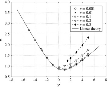
Wave speed
 $c$
in terms of the vorticity
 $\unicode[STIX]{x1D6FE}$
, for several values of
 $\unicode[STIX]{x1D700}$
. The solid line represents the dispersion relation for linear theory (A 1).

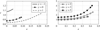
Wave propagation speed
 $c$
as a function of
 $\unicode[STIX]{x1D700}$
for different values of
 $\unicode[STIX]{x1D6FE}$
. For each value of
 $\unicode[STIX]{x1D6FE}$
, the curves are drawn up to
 $\unicode[STIX]{x1D700}_{max}$
.

In this appendix, we briefly review the effect of vorticity on the wave profiles and wave speeds, and their dependence on the wave height–wavelength aspect ratio,
 $\unicode[STIX]{x1D700}=H/\unicode[STIX]{x1D706}$
. The dispersion relation for linear waves is given by
 $$\begin{eqnarray}c=-b\unicode[STIX]{x1D6FE}+\frac{1}{2k}\left(\unicode[STIX]{x1D6FE}\tanh (k)\pm \sqrt{4k\tanh (k)+\unicode[STIX]{x1D6FE}^{2}\tanh ^{2}(k)}\right),\end{eqnarray}$$
where the depth has been fixed to unity. For waves in intermediate depth (
 $k=1$
), figure 11 shows the dependence of wave speed on vorticity for a range of
 $\unicode[STIX]{x1D700}$
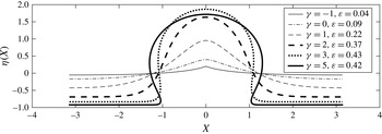
. For a given amplitude, there is a minimum value of vorticity that can support waves of that amplitude, but no maximum value: the vorticity can be arbitrarily large. In the limit of large vorticity, one obtains the exotic ‘disc’ profiles which limit to a fluid in rigid-body rotation. In figure 12, the curves for the wave speed as a function of amplitude are given at fixed vorticity values. Typical wave profiles for strongly nonlinear waves are shown in figure 13.
Wave profiles for the vorticity values of
 $\unicode[STIX]{x1D6FE}$
listed above and the corresponding maximum aspect ratio
 $\unicode[STIX]{x1D700}=\unicode[STIX]{x1D700}_{max}$
.