Introduction
Factors controlling seabird distributions are scale-dependent. At mega-scales (> 3000 km) the open ocean is heterogeneously structured with distinct biogeographical provinces (Ainley et al. Reference Ainley, Ribic and Fraser1994). Over macro-scales (1000–3000 km), physical factors such as sea-surface temperature (SST) and salinity separate hydrographic fronts, which form zones of enhanced primary and secondary production (Ainley et al. Reference Ainley, Ribic and Fraser1994, Chown et al. Reference Chown, Gaston and Williams1998, Bost et al. Reference Bost, Cotté, Bailleul, Cherel, Charrassin, Guinet, Ainley and Weimerskirch2009). At meso-scales (100–1000 km), biological factors become more important and correlations with prey more likely (e.g. Chown et al. Reference Chown, Gaston and Williams1998), although tracking studies show the importance of physical features to many top predators at these scales (Bost et al. Reference Bost, Cotté, Bailleul, Cherel, Charrassin, Guinet, Ainley and Weimerskirch2009). Variability increases when spatial scales are reduced due to stochasticity in physical and biological factors, and seabirds may use physical factors as cues to locate areas with enhanced probabilities of locating prey (Pakhomov & McQuaid Reference Pakhomov and McQuaid1996, Bost et al. Reference Bost, Cotté, Bailleul, Cherel, Charrassin, Guinet, Ainley and Weimerskirch2009). However, at a local scale seabirds must search directly for their preferred prey (Fraser & Ainley Reference Fraser and Ainley1986, Ballance et al. Reference Ballance, Pitman and Reilly1997), using visual or scent cues (Nevitt et al. Reference Nevitt, Veit and Kareiva1995). Temporal scales show a similar hierarchy although, at least at high latitudes, the strongest signal occurs seasonally rather than at longer time scales (Ainley et al. Reference Ainley, Ribic and Fraser1994, Ribic et al. Reference Ribic, Ainley, Ford, Fraser, Tynan and Woehler2011).
In the Southern Ocean, sea temperature and ice cover play important roles in structuring latitudinal differences in seabird communities (Abrams Reference Abrams1985, Ainley et al. Reference Ainley, Ribic and Spear1993), evident in the fairly uniform circumpolar distributions of birds associated with ice, ice-edge and open water habitats (Veit & Hunt Reference Veit and Hunt1991, Ribic et al. Reference Ribic, Ainley, Ford, Fraser, Tynan and Woehler2011). The seasonal marginal ice zone (MIZ) supports algal blooms (Froneman & Perissinotto Reference Froneman and Perissinotto1996) as well as larval and adult stages of Antarctic krill Euphausia superba Dana (Smetacek & Nicol Reference Smetacek and Nicol2005), fish, crustaceans and squid (Ainley et al. Reference Ainley, Ribic and Spear1993, Ainley et al. Reference Ainley, Jacobs, Ribic and Gaffney1998, Croxall et al. Reference Croxall, Trathan and Murphy2002). To understand which environmental factors control seabird distributions many studies have aggregated species into foraging guilds to relate guild distributions to physical features (e.g. Griffiths et al. Reference Griffiths, Siegfried and Abrams1982, Abrams Reference Abrams1985, Pakhomov & McQuaid Reference Pakhomov and McQuaid1996, Hyrenbach et al. Reference Hyrenbach, Veit, Weimerskirch, Metzl and Hunt2007). Such groupings can obscure the individual distributional response of a species, and their utility is questionable given considerable plasticity in the diets of many seabird species (Marchant & Higgins Reference Marchant and Higgins1990). Species behave individually in response to their needs, largely independent of the distribution of other species (Veit & Hunt Reference Veit and Hunt1991), and interspecific interactions apparently have little effect on the ranges of most species (but see Ribic et al. Reference Ribic, Ainley, Ford, Fraser, Tynan and Woehler2011).
A more informative approach to understanding seabird community structure at sea is to correlate species abundances with environmental factors (Ainley et al. Reference Ainley, Ribic and Fraser1994, Ribic et al. Reference Ribic, Ainley, Ford, Fraser, Tynan and Woehler2011), ideally combining at-sea data with tracking studies of individual predators (Bost et al. Reference Bost, Cotté, Bailleul, Cherel, Charrassin, Guinet, Ainley and Weimerskirch2009). Ribic et al. (Reference Ribic, Ainley, Ford, Fraser, Tynan and Woehler2011) found predictable seasonal assemblages of seabirds at a coarse scale in the Pacific Ocean and Indian Ocean sectors of the Southern Ocean. They compared seabird communities in three broad latitudinal zones: the high Antarctic south of the Southern Antarctic Circumpolar Current Front (SACCF, the southern boundary of the Antarctic Circumpolar Current), the low Antarctic between the SACCF and the Antarctic Polar Front (APF), and the sub-Antarctic north of the APF. However, they deliberately omitted data from frontal zones to “avoid any mixing of species along water mass boundaries” (Ribic et al. Reference Ribic, Ainley, Ford, Fraser, Tynan and Woehler2011, p. 1698) and did not allow the observations at sea to define bird assemblages. Ribic et al. (Reference Ribic, Ainley, Ford, Fraser, Tynan and Woehler2011) also contrasted summer (October–March) and winter (April–September) seabird communities, ignoring within-season variation in seabirds.
In this study, we use multiple regression models to describe spatial seabird distribution patterns in the African sector of the Southern Ocean. We report how seabird assemblages across the region vary in relation to physical factors (frontal systems and sea ice extent) and compare seabird distribution patterns between early and late summer seasons in two years to demonstrate consistent patterns across years. We show that the SACCF is a biogeographical boundary for seabirds in late summer, due to an influx of birds south of the SACCF.
Materials and methods
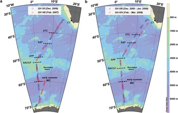
The study area was the Good Hope (GH) transect between Cape Town (34°S, 18°E) and the Antarctic ice shelf (70°S, 7°W). This meridional transect has been surveyed twice annually since 2004 (see Ansorge et al. Reference Ansorge, Speich, Lutjeharms, Goni, Rautenbach, Froneman, Rouault and Garzoli2005). We collected data from the SA Agulhas during two summers, with two transects per year, in the early and late season (Fig. 1a & b). The early summer transects were from 8–17 December 2006 (GH VII) and 23 December 2008–3 January 2009 (GH XIII), and the late summer transects from 5–14 February 2007 (GH VIII) and 22 February–2 March 2009 (GH XIV). The predetermined cruise track represented a non-randomised transect from a vessel of opportunity. Seabird observations were confined to deep, oceanic waters (> 1000 m deep) to minimize the confounding effects of bathymetry and proximity to land.
Seabird observations along the Good Hope transect in the Atlantic sector of the Southern Ocean during the summers of a. 2006–07, and b. 2008–09 in relation to oceanic fronts: STC = Subtropical Convergence, SAF = Sub-Antarctic Front, APF = Antarctic Polar Front, SACCF = Southern Antarctic Circumpolar Current Front, MIZ = marginal ice zone. Each circle depicts a continuous 60-min survey sample.

Abiotic data collection
We identified the positions of oceanographic fronts via their surface and subsurface (200 m) temperature and salinity expressions. Four major fronts were recognized: the Subtropical Convergence (STC), Sub-Antarctic Front (SAF), Antarctic Polar Front (APF) and Southern Antarctic Circumpolar Current Front (SACCF), often referred to as the southern boundary of the Antarctic Circumpolar Current or the Antarctic Divergence (Ansorge et al. Reference Ansorge, Speich, Lutjeharms, Goni, Rautenbach, Froneman, Rouault and Garzoli2005, Bost et al. Reference Bost, Cotté, Bailleul, Cherel, Charrassin, Guinet, Ainley and Weimerskirch2009, Ribic et al. Reference Ribic, Ainley, Ford, Fraser, Tynan and Woehler2011). However, we also analysed our data into three major water masses as defined by Ribic et al. (Reference Ribic, Ainley, Ford, Fraser, Tynan and Woehler2011): high Antarctic = south of the SACCF, low Antarctic = between the SACCF and the APF, sub-Antarctic = between the APF and the STC, to which we added temperate = north of the STC. Fronts were detected by deploying expendable bathythermographs (XBTs) to produce temperature profiles every 15 nautical miles (nm), increasing in frequency to every 10 nm across frontal regions. The northern extent of the pack ice (the MIZ) formed a physical boundary that retreated polewards during summer. In early summer surveys it occurred at around 60°S. By the late summer surveys very little if any sea ice was encountered other than occasional ice bergs. Maps of tracks and ocean structure were created in Ocean Data View v4 (Schlitzer Reference Schlitzer2009). Abiotic data were recorded hourly from the start of each survey session: date and time, position, ship's speed and heading, wind direction and speed, SST, sea state (on a scale of 1 (calm) to 5 (very rough)), percentage cloud cover and percentage ice cover within each 300 x 300 m count area (see below).
Seabird counts
We counted seabirds during daylight hours from the bridge or monkey deck (16–18.5 m above sea level), depending on weather conditions, using a 90° field of view to the side of the bow with best visibility (glare or light dependent). We used a 300 x 300 m survey box, effectively creating a continuous 300 m wide strip transect following Tasker et al. (Reference Tasker, Jones, Dixon and Blake1984). All birds sitting on the water or ice in the transect area were counted. However, we only counted flying birds sampled during an ‘instant’ scan at the start of each observation minute to reduce biases caused by flux of flying birds through the transect (Tasker et al. Reference Tasker, Jones, Dixon and Blake1984). On the few occasions when the ship's speed fell below 7 knots, we only counted flying birds every two minutes to equalize survey effort (Tasker et al. Reference Tasker, Jones, Dixon and Blake1984). Observations of birds following the ship preceded all survey sessions. We excluded from steaming counts all birds circling the ship as well as new birds obviously attracted by the ship (i.e. birds observed to approach the vessel from beyond the 300 m-wide transect area). We reduced the attractiveness of the vessel to ship-following birds by ensuring that food scraps were discarded only after each day's survey effort was complete.
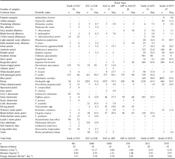
Although small and inconspicuous species are under-represented in strip transect counts (especially when only one observer was on duty), seabird numbers generally were too great to use a distance-based approach to estimate densities. We also did not attempt to compensate for differences in detection rates linked to environmental conditions (e.g. sea state). Detection probabilities were improved by scanning with binoculars every minute, and observer bias was limited by using the same two observers within each voyage. Some seabirds were not identified to species level due to identification issues at sea: prions, giant petrels, yellow-nosed albatrosses, diving petrels, and Sterna terns were pooled (Table I). Seabird density was estimated from the survey area (the product of speed over ground and survey width). Biomass calculations were based on average species mass values taken from Marchant & Higgins (Reference Marchant and Higgins1990) and Hockey et al. (Reference Hockey, Dean and Ryan2005). Energy demand was estimated from allometric equations for field metabolic rate in Nagy et al. (Reference Nagy, Girard and Brown1999).
Abundance and frequency (freq) of occurrence (%) of seabird species observed along four transects across the Atlantic sector of the Southern Ocean between Cape Town and Antarctica, collated into 60 min sample sizes.

STC = Subtropical Convergence, SAF = Sub-Antarctic Front, APF = Antarctic Polar Front, and SACCF = Southern Antarctic Circumpolar Current Front.
Multivariate analyses of seabird assemblages
Seabird abundance (biotic) and environmental (abiotic) data were aggregated into continuous 1-hour blocks (henceforth samples), corresponding to c. 20 km transects. We a priori categorized samples by year (2006–07, 2008–09) and season (early or late summer). To test the hypothesis that large-scale hydrographic features structure seabird assemblages, we also categorized samples into six water masses, based on in situ definition of oceanic fronts and the early summer northernmost extent of sea ice (60°S). Observation effort was comparable between years and water masses (Table S1, which will be found at http://dx.doi.org/10.1017/S0954102013000138).
We analysed the biotic count data for patterns before attempting to relate it to the abiotic data. Our multi-species or species-by-sample data are multivariate in character and were analysed using non-parametric multivariate techniques in PRIMER v6 (Clarke & Gorley Reference Clarke and Gorley2006), including PERMANOVA+ (Anderson et al. Reference Anderson, Gorley and Clarke2008), packages designed specifically to analyse community structures and their environmental correlates. Similarities were calculated using the Bray-Curtis coefficient, which is not affected by joint absences and gives more weight to abundant species. However, seabird abundances were fourth-root transformed to allow scarce species to contribute to the similarities between samples.
An agglomerative, hierarchical cluster analysis produced a dendrogram by linking group averages of sample resemblances. A permutation based similarity profile test (SIMPROF) of the cluster hierarchy found groupings with no significant (P < 0.005) internal structure (999 permutations). This method avoids over-interpretation of within-group structure where none exists (Clarke & Gorley Reference Clarke and Gorley2006). A non-metric multi-dimensional scaling (MDS) ordination of samples allowed a two-dimensional visualization of the multi-dimensional dataset, with stress values (0–1) giving a measure of the adequacy of the ordination at the reduced number of dimensions. Values < 0.2 are acceptable, although < 0.1 is ideal (Clarke & Warwick Reference Clarke and Warwick2001, Quinn & Keough Reference Quinn and Keough2002). By comparing the cluster analysis dendrogram with an MDS ordination of SIMPROF-derived groupings, we increased confidence between the two ordination methods.
To test the null hypothesis of no difference in biotic structure between seasons and years, we used the permutational analysis of multivariate dispersions (PERMDISP) and the non-parametric analysis of variance (PERMANOVA) routines (Anderson et al. Reference Anderson, Gorley and Clarke2008). PERMDISP tests the homogeneity of multivariate dispersion between groups (9999 permutations). Distances between samples and their group centroid were compared with ANOVA F statistics, or t statistics for pair-wise levels of a factor. PERMANOVA tests for a location effect in non-parametric data by partitioning the variability according to a set experimental design. We used a three-way crossed design with the factors year, season and water mass, fitting each term only after taking into account all other terms in the model (Type III or partial sum of squares). Residuals were permuted under a reduced model. For each term in the model, a pseudo-F statistic was calculated and 9999 permutations provided significance. Estimates of components of variation were based on percentages from the underlying Bray-Curtis similarities and are analogous to univariate standard deviations (Anderson et al. Reference Anderson, Gorley and Clarke2008).
To find the subset of species which best reconstructed the multi-dimensional sample pattern, we used the BVSTEP method of the BEST routine (Clarke & Gorley Reference Clarke and Gorley2006). This method uses Spearman rank-based correlations (ρ) between two similarity matrices, with ρ > 0.95 considered a close to perfect match (Clarke & Warwick Reference Clarke and Warwick2001). We chose the convergent solution with the highest correlation from forward-stepping and random runs, re-starting 20 times with ten variables. The SIMPER routine determined which species best characterized the a priori season and water mass factors as well as the significant groupings from the SIMPROF test. When appropriate, we used a two-way crossed layout to remove the effect of an interacting factor found to be significant.
Linking seabird assemblages to the environment
We included variables that may have influenced the location of a seabird or our ability to detect a seabird because most variables contribute to some degree to both phenomena. The first 25 hours of transect counts from GH VII had incomplete environmental data and were excluded. For the remaining samples, we examined each abiotic variable for approximate normality and linearity using scatter plots and transformed certain variables to achieve more symmetrical distributions. Time of day (GMT), and percentage cloud and ice cover were arcsine transformed. Directional variables (ship's course and wind direction) were decomposed into ‘northness’ and ‘eastness’ using cosine and sine transformations, respectively (Clark et al. Reference Clark, Palmer and Clark1999). Right-skewed variables were modified with a square root transformation (sea state) or a natural log transformation (distance). A reverse natural log transformation effectively transformed the left-skewed SST variable (ln(24-SST)). Ln(Distance (km)) was derived from and highly correlated to ship's speed over ground, so the latter variable was dropped, giving 14 abiotic variables for all analyses. We retained longitude, despite its strong negative correlation with latitude (r = -0.87) and ln(24-SST) (r = -0.89), because it was below the usual cut-off of r = 0.95 (Clarke & Gorley Reference Clarke and Gorley2006).
We used the distance-based linear models (DISTLM) routine of PERMANOVA+ to model the relationship between seabird count data and abiotic predictor variables using a multiple regression model (Anderson et al. Reference Anderson, Gorley and Clarke2008), under the null hypothesis of no relationship between biotic and abiotic variables. This routine partitions variation in the dataset into each predictor variable. Marginal tests found variability in the responses explained by individual predictors. We set significance at P ≤ 0.01 to correct for inflated Type I errors. Model selection was based on conditional tests, which assessed the proportion of variability explained by individual predictors after fitting one or more other predictors based on 9999 permutations. To select the most parsimonious model, we compared the model from a step-wise selection procedure, using adjusted r 2 as the selection criterion, with models from a “best” selection procedure based on the Bayesian Information Criterion (BIC). The most parsimonious model was inspected with the distance-based redundancy analysis (dbRDA) routine of PERMANOVA+, which found linear combinations of predictor variables that explained the greatest proportion of variability in bird distributions.
Results
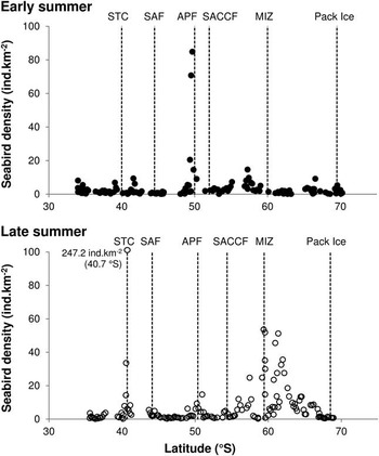
Seabird counts were made during 294 hours of transects, with roughly equal coverage across the four cruise legs (Table S1, which will be found at http://dx.doi.org/10.1017/S0954102013000138), recording 11 565 individuals from 37 taxa (Table I). Frontal positions during the voyages are shown in Fig. 1. In early summer we reached the seasonal MIZ at c. 60°S, but by late summer the MIZ had retreated to close to the ice shelf edge and was not represented in transect counts. Seabird densities were fairly consistent (CV ∼ 100%) in all water masses except sub-Antarctic waters (Table II), due to large aggregations of prions in some transects. In early summer, seabird densities peaked around the APF (50°S) and just north of the ice-edge at around 57.5°S (Fig. 2). By late summer, seabird densities shifted southward in response to retreating sea ice, with highest densities observed between 60 and 65°S (Fig. 2). This was reflected by a marked increase in average bird density in high Antarctic waters from early to late summer (Table II).
Densities of seabirds (birds km-2) in major oceanographic zones recorded in the African sector of the Southern Ocean (this study) compared with data from the Indian Ocean and Pacific Ocean sectors (from Ribic et al. Reference Ribic, Ainley, Ford, Fraser, Tynan and Woehler2011).

*Temperate waters not reported by Ribic et al. (Reference Ribic, Ainley, Ford, Fraser, Tynan and Woehler2011), see Methods for descriptions of zones.
Seabird densities observed along two early summer and two late summer transects during 2006–07 and 2008–09 in the Atlantic sector of the Southern Ocean. Frontal acronyms as in Fig. 1.

Seabird assemblages
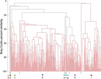
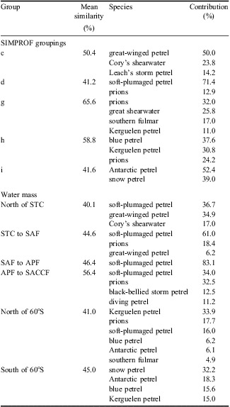
Clear evidence of structure within seabird assemblages was visible in the cluster analysis dendrogram, which showed five main groupings (Fig. 3). The SIMPROF derived groupings were not constrained a priori and thus incorporated differences in space (water masses) and over time (seasons, years). Group ‘c’ corresponded largely to samples in the warmer waters north of the STC, and was characterized by great-winged petrels, Cory's shearwaters and Leach's storm petrels (Table III). Group ‘i’ corresponded to samples in the coldest waters associated with ice located mainly south of 60°S, and was characterized by Antarctic and snow petrels (Table III). Group ‘d’ was the largest group and contained samples from all water masses between the STC and the SACCF. Only two taxa with wide latitudinal ranges characterized this group: prions and soft-plumaged petrels (Table III).
A dendrogram of Southern Ocean seabirds based on continuous 60-min samples. Similarities calculated using the Bray-Curtis coefficient on fourth-root transformed abundance data. Red lines indicate groupings with no significant internal structure (SIMPROF overall test, π = 3.49, P < 0.001). Five main SIMPROF groupings were found, arbitrarily labelled c, d, g, h and i.

Species characterizing groups of Southern Ocean seabirds. Species shown are cut off at 80% cumulative contribution. Groupings for the SIMPER analysis were defined on significant SIMPROF groupings (P < 0.005) from a cluster analysis, with only the five main SIMPROF groupings shown, as well as by a priori water mass categories, accounting for the effect of seasons. Within each group, similarity is mean Bray-Curtis similarity between pairs of samples.

STC = Subtropical Convergence, SAF = Sub-Antarctic Front, APF = Antarctic Polar Front, and SACCF = Southern Antarctic Circumpolar Current Front.
There was a distinct seasonal shift in seabird assemblages in waters south of the SACCF. The SACCF had little effect on bird assemblages in early summer, when waters between the SACCF and the northern limit of the MIZ (∼ 60°S) supported an assemblage similar to group ‘d’, and were incorporated into this group. Further south, the pack ice was characterized by the pagophilic ‘i’ group. By late summer, the sea ice had retreated to the proximity of Antarctica, and assemblages south of the SACCF were distinct from the broad ‘d’ group assemblage, with two distinct but fairly similar (> 35% similarity) assemblages. Group ‘g’, characterized primarily by prions and great shearwaters, occurred in waters between the SACCF and 60°S. Group ‘h’, characterized by blue and Kerguelen petrels, occurred in late summer waters south of 60°S. Thus, in late summer, the SACCF had strong separating power, splitting seabird assemblages between the STC and Antarctica.
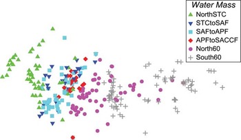
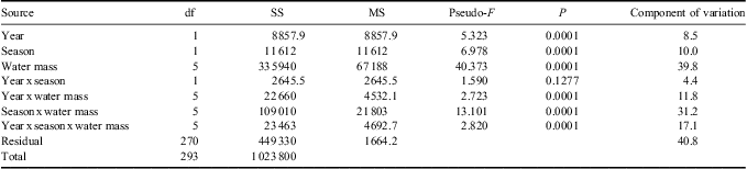
The five main cluster analysis groupings aligned along the x-axis of an MDS ordination of samples by water mass (Fig. 4). The PERMDISP analyses showed homogeneous sample dispersion between years (F 1,292 = 1.593, P = 0.298), but early summer samples were more dispersed than late summer samples (F 1,292 = 13.622, P < 0.001). Sample dispersions were heterogeneous between water masses (F 5,288 = 22.603, P < 0.0001) and differed between eight of the 15 water mass pairings (P < 0.01). Water mass, year and season explained almost 60% of variation in seabird assemblages, with water mass the most influential factor (39.8% of variation) followed by season (10.0%, Table IV). However, there were significant interaction effects between factors. Differences in the location of seasonal assemblages within the ‘STC to SAF’, ‘SAF to APF’, ‘North of 60°S’ and ‘South of 60°S’ water masses drove the interaction between season and water mass (P < 0.01). The interaction between year and water mass was driven by shared locations in 2008–09 of the water mass pairing ‘STC to SAF’ and ‘SAF to APF’ and the pairing ‘STC to SAF’ and ‘APF to SACCF’ (P < 0.01), as well as different assemblage locations between years within the ‘North of STC’ and ‘South of 60°S’ water masses (P < 0.01). Interactions that did not involve water mass were not significant, suggesting that water mass explained most variability in seabird assemblages.
A multi-dimensional scaling ordination of Southern Ocean seabird assemblages categorized a priori by water mass: north of the STC (North STC), the STC to the SAF (STC to SAF), the SAF to the APF (SAF to APF), the APF to the SACCF (APF to SACCF), the SACCF to 60°S (North60) and south of 60°S (South60). Frontal acronyms as in Fig. 1. 2D stress = 0.1.

Multivariate test of location differences (PERMANOVA) in Southern Ocean seabird assemblages. The analysis used a three-way crossed design with all factors fixed.

df = degrees of freedom, SS = sum of squares, MS = mean square.
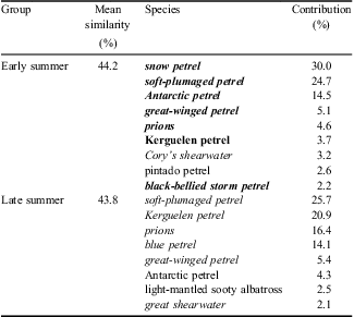
Despite similar mean sample similarities within each season (44%), the species characterizing each season differed (Table V). Snow petrels, Cory's shearwaters, pintado petrels and black-bellied storm petrels characterized early summer, and Antarctic petrels were more abundantly observed in early summer due to their pagophilic nature and the greater early summer extent of the MIZ. Blue petrels, light-mantled sooty albatrosses and great shearwaters characterized late summer, and there were marked increases in Kerguelen petrels and prions at this time (Table V). Soft-plumaged and great-winged petrels had equal contributions in both early and late summer.
Species characterizing seasonal assemblages of Southern Ocean seabirds (cut-off at 90% cumulative contributions). The SIMPER analysis accounted for the effect of water masses. Within each season, similarity is mean Bray-Curtis similarity between pairs of samples. Italicised species are those that together best represented the multi-dimensional species pattern for that season, based on all species (ρ = 0.95 for each season). Bold species are those that together best represented the entire multi-dimensional species pattern, based on all species (ρ = 0.95).

Seabird habitats
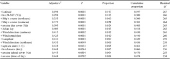
Marginal tests of DISTLM showed all variables except time of day to be significantly related to the seabird data, ignoring other variables (P < 0.01). Specifically, latitude explained 19.7% of variability in seabird community structure, followed by longitude (12.4%), SST (11.8%), ice cover (6.5%), distance (5.4%) and heading (northness) (5.3%), with remaining variables individually explaining < 5% of the variability. The 14 abiotic variables in the most parsimonious model explained 47.4% of the total variation (adjusted r 2 = 0.444; Table VI). After fitting latitude, SST maximally improved the adjusted r 2 value in the DISTLM step-wise selection procedure, explaining a further 10.3% of the variation. The first five variables together explained 40.5% of the variation, with additional variables each explaining < 1.5%. The top five variables, along with Julian Day, provided the model with the lowest BIC value (2088.1), and were deemed to offer the most parsimonious model, accounting for 41.8% of variation in the dataset.
Multiple regression model of the relationship between seabird abundances and abiotic predictor variables (distance-based linear models (DISTLM) sequential test, based on a step-wise selection procedure). Sample similarities were calculated using the Bray-Curtis similarity coefficient on fourth-root transformed abundance data.

df = degrees of freedom, SST = sea surface temperature.
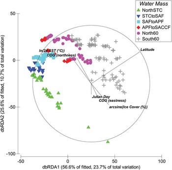
The first two axes of a dbRDA ordination captured 82.1% of the variation in the fitted DISTLM model (Fig. 5), but only 34.3% of total variation. Latitude had the strongest effect on seabird assemblage structure, corresponding to latitudinally segregated water masses, followed by seasonal changes (driven primarily by SST and ice cover). Despite the strong positive correlation (r = 0.80) between latitude and SST, they drove different aspects of variation in seabird assemblages. Variability within water masses was especially evident for samples from the water masses ‘North of the STC’, ‘North of 60°S’ and ‘South of 60°S’, which exhibited the greatest y-axis variation. The pattern in the 2D constrained dbRDA was largely similar to the 2D pattern in an unconstrained principal co-ordinates analysis (PCO, not shown), indicating that the model broadly captured the patterns in the dataset (Anderson et al. Reference Anderson, Gorley and Clarke2008).
A distance-based redundancy analysis (dbRDA) of the six predictor variables from a parsimonious distance-based linear model (DISTLM) that explained the greatest variation in Southern Ocean seabird abundance patterns. Vectors correspond to multiple partial correlations of predictor variables with the two axes, showing the direction and strength of the effect of the predictor variable. Water masses labelled as in Fig. 4.

Discussion
The study was conducted in an area distant from major seabird breeding sites in the Southern Ocean. The only island within 1000 km of the transect is Bouvetøya, which supports relatively small seabird populations (Watkins Reference Watkins1981), and the coastline of Dronning Maud Land, which lacks ice-free land where coastal breeding species can breed (Marchant & Higgins Reference Marchant and Higgins1990). This might account for the low densities of birds in our study (3–11 birds km-2) compared to the 20–30 birds km-2 reported in summer from Antarctic and sub-Antarctic waters in other parts of the Southern Ocean by Ribic et al. (Reference Ribic, Ainley, Ford, Fraser, Tynan and Woehler2011) (Table II). This difference is even more marked than it might appear from Table II, because Ribic et al. (Reference Ribic, Ainley, Ford, Fraser, Tynan and Woehler2011) excluded frontal zones from their data, and bird densities generally peaked across fronts (Fig. 2). The paucity of nearby large breeding populations might also explain the lack of an increase in seabird abundance, biomass and energy demand at higher latitudes (cf. Ribic et al. Reference Ribic, Ainley, Ford, Fraser, Tynan and Woehler2011). Breeding penguins in particular tend to have fairly limited foraging ranges, and given their large size they contribute disproportionately to biomass estimates of seabirds in the Southern Ocean.
One benefit of working in an area distant from major breeding colonies is that most seabirds observed were likely to be foraging or moving between foraging areas, rather than commuting to and from breeding colonies. This probably enhanced our ability to detect coherent patterns of seabird distribution in relation to a simple suite of environmental factors, and reduced the variance in density estimates compared to Ribic et al. (Reference Ribic, Ainley, Ford, Fraser, Tynan and Woehler2011). It also might explain the late summer increase in the abundance of birds that breed early in the summer season (e.g. Kerguelen petrels and prions). This pattern is probably driven by an influx of post-breeding adults.
Observed summer patterns of seabird distributions were broadly similar to those found in the Pacific Ocean and Indian Ocean sectors of the Southern Ocean (Ribic et al. Reference Ribic, Ainley, Ford, Fraser, Tynan and Woehler2011). Regional differences, such as the paucity of sooty shearwaters and absence of short-tailed shearwaters Puffinus tenuirostris (Temminck) from the south-west Atlantic Ocean, have been attributed to competition with high densities of Antarctic petrels and Pygoscelis penguins in this region (Ribic et al. Reference Ribic, Ainley, Ford, Fraser, Tynan and Woehler2011). However, distance from breeding sites in early summer and the late summer influx of great shearwaters offer more plausible explanations for their scarcity in the central Atlantic sector of the Southern Ocean. Our within-season sampling allowed differentiation between the less diverse early summer assemblage and more diverse late summer assemblage, especially at higher latitudes. This contrasts with the analysis of Ribic et al. (Reference Ribic, Ainley, Ford, Fraser, Tynan and Woehler2011), which pooled data throughout summer (October–March).
The structure of seabird communities south of Africa was best explained by latitude and season. Both these variables reflect changes in physical factors within water masses, with resultant impacts on the distribution and abundance of prey species. Sea-surface temperature plays a key role in determining the biogeography and biogeochemistry of the Southern Ocean (Gibbons Reference Gibbons1997), especially north of the STC. Ice cover was important in the south of the region, where tolerance of physical conditions starts to outweigh biotic factors (Ainley et al. Reference Ainley, Ribic and Spear1993, Ballance et al. Reference Ballance, Pitman and Reilly1997). Taken together, the seasonal variation in SST and ice cover were the most important physical factors determining summer seabird assemblages, which agrees with previous studies in other regions of the Southern Ocean (Ainley et al. Reference Ainley, Ribic and Fraser1994, Ribic et al. Reference Ribic, Ainley, Ford, Fraser, Tynan and Woehler2011). Patterns were consistent across years, suggesting that seabird assemblage structure is relatively predictable in this region. However, our model explained less than half the variation in seabird distribution patterns, probably as a result of the importance of factors operating at finer spatial scales than those included in the model (e.g. prey distribution, water transparency etc.).
On a macro-scale, the position of oceanic fronts and the northern extent of the pack ice (the MIZ) constrained the distributions of many seabird species. Similar assemblage structuring by fronts was found for zooplankton in the Atlantic and Indian oceans (Pakhomov & McQuaid Reference Pakhomov and McQuaid1996) and for seabirds in the south-west Atlantic (Veit Reference Veit1995). The northern limit of the pack ice forms probably the most consistent boundary to seabirds, with a distinct ice-associated assemblage to the south, characterized by Antarctic and snow petrels as well as ice-associated penguins (Ribic et al. Reference Ribic, Ainley, Ford, Fraser, Tynan and Woehler2011, and references therein). This community was absent from our samples in late summer when the pack ice had retreated close to the continent, but it persists by tracking the contracting and expanding ice zone (Ainley et al. Reference Ainley, Ribic and Spear1993, Croxall et al. Reference Croxall, Steele, McInnes and Prince1995). Melting sea ice releases algae that seed phytoplankton blooms maintained by the relative stability of the freshwater melt (Fraser & Ainley Reference Fraser and Ainley1986, Veit & Hunt Reference Veit and Hunt1991, Froneman & Perissinotto Reference Froneman and Perissinotto1996). These blooms support Antarctic krill, copepods and amphipods attracting large numbers of seabirds (Smetacek & Nicol Reference Smetacek and Nicol2005). Pagophilic species desert this area as summer progresses, despite sharing a common diet with the species that replace them (Ainley et al. Reference Ainley, Ribic and Spear1993), apparently because they are adapted to feeding in the pack ice zone where waves are suppressed, preventing dynamic soaring (Ainley et al. Reference Ainley, Ribic and Spear1993, Ainley et al. Reference Ainley, Ribic and Fraser1994).
The STC also represents a strong boundary to seabirds, acting as a biogeographical division between the Southern Ocean and warmer subtropical waters. The waters immediately north of the STC are highly productive in both early and late summer (Laubscher et al. Reference Laubscher, Perissinotto and McQuaid1993, Barange et al. Reference Barange, Pakhomov, Perissinotto, Froneman, Verheye, Taunton-Clark and Lucas1998). Nevertheless, seabird densities generally were low in oceanic waters north of the STC (Table I), but we observed high seabird densities at the STC in late summer, especially in 2008–09 when prions dominated observations (Fig. 2). However, not all fronts separate distinct zooplankton communities (Pakhomov et al. Reference Pakhomov, Perissinotto, McQuaid and Froneman2000) or seabird assemblages (Bost et al. Reference Bost, Cotté, Bailleul, Cherel, Charrassin, Guinet, Ainley and Weimerskirch2009). The SAF and APF had less influence over seabird communities than the STC and ice-edge, and there was no structure across the SACCF in early summer. These waters support a diverse group of seabirds between the STC and the pack ice-edge in early summer, when previous studies also have found little difference in the composition of seabird and zooplankton communities (Pakhomov & McQuaid Reference Pakhomov and McQuaid1996). Within this broad region, there was considerable variation in seabird abundance, presumably linked to localized concentrations of prey (e.g. Hyrenbach et al. Reference Hyrenbach, Veit, Weimerskirch, Metzl and Hunt2007). We observed a large peak in seabird numbers (dominated by prions) at the APF in early summer, when the APF shows enhanced productivity (Laubscher et al. Reference Laubscher, Perissinotto and McQuaid1993, Guinet et al. Reference Guinet, Koudil, Bost, Durbec, Georges, Mouchot and Jouventin1997), often attracting large numbers of prions (Ribic et al. Reference Ribic, Ainley, Ford, Fraser, Tynan and Woehler2011). Productivity along the SAF is more uniform than the APF and at least sometimes forms a biogeographical boundary to zooplankton (Pakhomov et al. Reference Pakhomov, Perissinotto, McQuaid and Froneman2000).
In contrast to early summer, we found two seabird assemblages between the SACCF and the pack ice in late summer, when open water extends virtually to the ice shelf edge. These assemblages segregated around the position of the maximum northern extent of sea ice at c. 60°S. The position of the SACCF affects coastal currents and sea ice, which in turn influence zooplankton abundance and distribution (Nicol et al. Reference Nicol, Pauly, Bindoff, Wright, Thiele, Hosie, Strutton and Woehler2000). During early summer, prions were characteristic of the area of open water between the SACCF and the MIZ (60°S), but in late summer blue and Kerguelen petrels, great shearwaters and southern fulmars characterized this zone and the expanding zone of open water south of 60°S. This seasonal ‘invasion’ of species into the open water north of the ice-edge occurs around the continent (Veit & Hunt Reference Veit and Hunt1991, Ainley et al. Reference Ainley, Ribic and Fraser1994, Ribic et al. Reference Ribic, Ainley, Ford, Fraser, Tynan and Woehler2011). It would be interesting to know the age and breeding status of these birds. Kerguelen and blue petrels have finished breeding by this time, but great shearwaters and most southern fulmars have not (Marchant & Higgins Reference Marchant and Higgins1990), and it is unknown whether some adults provisioning chicks feed in these waters.
In summary, seabird community patterns were similar between years suggesting a measure of predictability, although further sampling is needed to confirm interannual patterns. Two gradients drove seabird assemblages in the study area: a spatial gradient, reflecting oceanographic fronts, and a seasonal one driven by variation in SST and ice cover. The STC and pack-ice-edge posed consistent boundaries to seabirds, dividing distinct assemblages throughout summer. By comparison, the productive water adjacent to the sea ice experienced a shift in seabirds as the ice retreated during summer, as birds typically found further north dispersed into the area. Seasonality was most evident in assemblages north of the STC and in those associated with the ice-edge.
Acknowledgements
We thank Dennis Weir, Clifford Dorse and Suretha van Rooyen for assistance with data collection, and the other scientific personnel, officers and crew of the SA Agulhas for their support at sea. Two anonymous reviewers greatly improved previous drafts of this paper. Financial and logistical support was provided by the South African National Antarctic Programme and the University of Cape Town.