1 Introduction
The presence of rotary motion is an important factor in determining the unsteady forces on a wing. Compared to the more conventional case of a translating wing, a rotating wing is subject to several physical mechanisms, including spanwise flow, vortex tilting and Coriolis effects, that complicate the prediction of aerodynamic forces. This has been shown to be particularly important for wings with substantial flow separation. When a wing undergoes a rapid translation at high angle of attack, flow will tend to separate near the leading edge and roll up into a leading-edge vortex (LEV), which convects into the wake of the wing. For similar velocities on a rotating wing, the motion of the wing still causes separation, but rather than convecting into the wake, the LEV remains stable over a certain portion of the span (Lentink & Dickinson Reference Lentink and Dickinson2009b ). The prolonged attachment of the LEV can significantly change the force history of the wing over time (Usherwood & Ellington Reference Usherwood and Ellington2002; Usherwood Reference Usherwood2009; Jones & Babinsky Reference Jones and Babinsky2010; Schlueter et al. Reference Schlueter, Jones, Granlund and Ol2014; Wojcik & Buchholz Reference Wojcik and Buchholz2014a ; Manar et al. Reference Manar, Mancini, Mayo and Jones2016), and thus, many researchers have sought to understand which features of a rotating wing are responsible for stabilization of the LEV (Jardin & David Reference Jardin and David2014; Medina & Jones Reference Medina and Jones2016; Jardin Reference Jardin2017).
Several hypotheses have been put forward as a means of explaining the behaviour of LEVs on rotating wings. The first and perhaps most intuitive is related to flow along the wing span. Studying a model insect wing in hover, Ellington et al. (Reference Ellington, van den Berg, Willmott and Thomas1996) posited that flow along the wing span acts to ‘drain’ vorticity from the LEV, thereby preventing it from growing beyond a critical size. This hypothesis was seconded by van den Berg & Ellington (Reference van den Berg and Ellington1997) and is analogous to a similar phenomenon observed on high-speed delta wings (Polhamus Reference Polhamus1966). Recent experimental efforts, however, are at odds with Ellington’s original idea, and many studies have suggested that spanwise flow alone is not a sufficient explanation for the stability of LEVs on rotating wings (Birch & Dickinson Reference Birch and Dickinson2001; Beem, Rival & Triantafyllou Reference Beem, Rival and Triantafyllou2012; Wong, Kriegseis & Rival Reference Wong, Kriegseis and Rival2013; Wong & Rival Reference Wong and Rival2015). Wojcik & Buchholz (Reference Wojcik and Buchholz2014b ), in particular, quantified the magnitude of vorticity transport on a rotating wing and concluded that the effect of spanwise flow, although non-zero, is unlikely to match the rapid growth rate of the LEV.
A more promising hypothesis was posited by Lentink & Dickinson (Reference Lentink and Dickinson2009a ,Reference Lentink and Dickinson b ) in a series of experimental works testing wings in pure rotation. The authors proposed that the magnitude of the Coriolis force, not spanwise flow, is often the deciding factor in the stability of the LEV, and the relative importance of rotation can be predicted from the local Rossby number. Equation (1.1) provides a formal definition of the Rossby number, typically defined as the ratio of inertial to Coriolis force at a point on the wing:
 $$\begin{eqnarray}Ro=\frac{U}{L\unicode[STIX]{x1D6FA}}.\end{eqnarray}$$
In (1.1),
 $\unicode[STIX]{x1D6FA}$
represents the angular velocity of the wing,
 $U$
represents a characteristic velocity and
 $L$
represents a characteristic length. Lentink & Dickinson (Reference Lentink and Dickinson2009a
) proposed using the chord (
 $c$
) as a characteristic length scale and the local rotation velocity (
 $\unicode[STIX]{x1D6FA}r$
) as a characteristic velocity scale. The resulting expression for Rossby number,
 $Ro=r/c$
, where
 $r$
is the local distance along the blade span, has been positively correlated with stability of the LEV in a number of studies (Wolfinger & Rockwell Reference Wolfinger and Rockwell2014; Lee, Lua & Lim Reference Lee, Lua and Lim2016; Bhat et al.
Reference Bhat, Zhao, Sheridan and Hourigan2019). A local Rossby number of
 $O(1)$
frequently appears in these works as a criterion for LEV stability on rotating wings in hover.
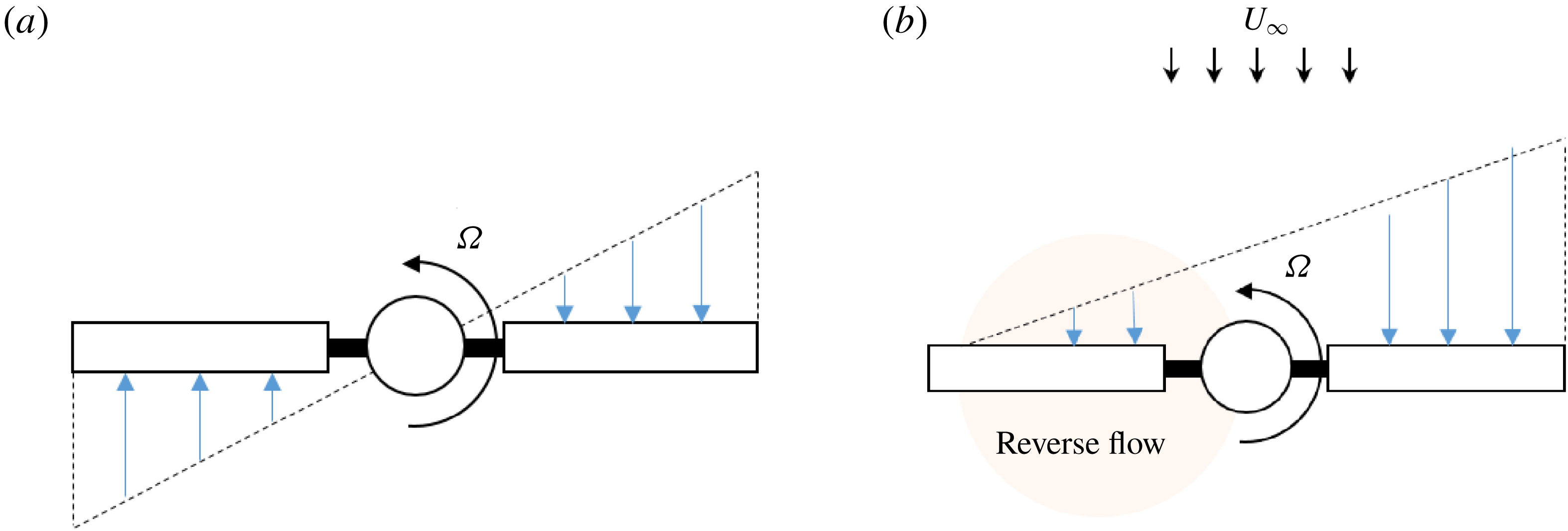
The velocity distribution on a rotating wing in hover (a) and a rotating wing in forward flight (b). Reverse flow, highlighted in orange, occurs when the forward flight velocity (
 $U_{\infty }$
) exceeds the local rotational velocity (
 $\unicode[STIX]{x1D6FA}r$
) during the wing’s retreat.

The Rossby number is a promising metric for predicting the importance of rotation, but its current use is limited to the case of a rotating wing in hover. The effect of a forward flight velocity, which arises in many practical applications, is not well understood. The problem is compounded by the fact that the aerodynamic environment of a rotating wing in forward flight is significantly more complex than one in hover. A rotating wing in forward flight, for instance, is continuously reorienting itself relative to the forward flight velocity, so the local free stream oscillates in time. This includes a region of reverse flow, or trailing-edge to leading-edge flow, that develops when the wing is ‘retreating’ (see figure 1). Contrary to rotating wings in hover, the local free stream in reverse flow increases as one moves inboard along the span, reversing the direction of spanwise gradients. It is thus particularly uncertain whether the conclusions related to rotating wings in hover hold in the reverse flow region. Harbig, Sheridan & Thompson (Reference Harbig, Sheridan and Thompson2014) provided a detailed map of vortex stability over various advance ratios and aspect ratios for kinematics that included reverse flow, but the authors did not directly address changes in the two-dimensional (2-D) and three-dimensional (3-D) vortex dynamics. Granlund, Ol & Jones (Reference Granlund, Ol and Jones2016) performed experiments that mirror the unsteady free stream experienced by a rotating wing in forward flight, but the authors did not investigate how their results would change in the presence of rotation.
The current work will attempt to quantify the role of 2-D and 3-D flow physics in the evolution of vortices in the reverse flow region of a rotating wing in forward flight. In the sections that follow, attention will be paid to whether the Rossby number criterion, which has been shown to provide an intuitive sense of the role of rotation on a wing in hover, holds in the presence of a large forward flight velocity. To more properly represent the reverse flow region, the local Rossby number will be adjusted according to
 $$\begin{eqnarray}Ro=\frac{U_{r,avg}}{c\unicode[STIX]{x1D6FA}},\end{eqnarray}$$
where
 $U_{r,avg}$
represents the average free-stream velocity experienced by a certain spanwise position of the wing in the reverse flow region. The specific goals of this work are (i) to assess whether (1.2) can predict the relative magnitude of Coriolis forces on a rotating wing in forward flight, and (ii) to determine whether Coriolis forces are the defining characteristic of vortex stability in reverse flow, as they appear to be on a wing in hover.
2 Methodology
2.1 Rotor system
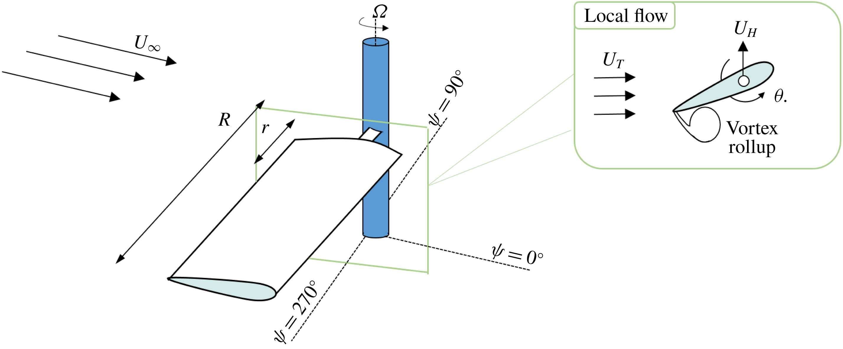
Problem statement: a rotating, sharp trailing-edged wing subject to a large forward flight velocity (
 $U_{\infty }$
).

The current work investigates the role of 3-D vortex dynamics via numerical simulation of an articulated rotor in forward flight. This particular model was chosen to reflect certain practical applications, such as full-scale helicopters, rotary unmanned aerial vehicles (UAVs) and vertical-axis wind turbines, that employ articulation to maximize thrust for a given flight condition. Since the motions of an articulated blade are somewhat unintuitive to visualize, this section will briefly familiarize the reader with the various motions of an articulated rotor in forward flight. As seen in figure 1, a rotor blade element in forward flight is subject to an unsteady variation in its local free-stream velocity due to the rotational and translational components of its motion. The local blade-tangent velocity (
 $U_{T}$
) varies both temporally and spatially and can be defined according to
 $$\begin{eqnarray}U_{T}=\unicode[STIX]{x1D6FA}R(r/R+\unicode[STIX]{x1D707}\sin \unicode[STIX]{x1D713}),\end{eqnarray}$$
where
 $\unicode[STIX]{x1D707}$
is the advance ratio of the rotor (
 $\unicode[STIX]{x1D707}=U_{\infty }/(\unicode[STIX]{x1D6FA}R)$
), and
 $\unicode[STIX]{x1D713}$
represents a non-dimensional time in the blade’s revolution (
 $\unicode[STIX]{x1D713}=\unicode[STIX]{x1D6FA}t$
). On an articulated rotor, a blade element will simultaneously undergo oscillations in its pitch (
 $\unicode[STIX]{x1D703}$
) and flap velocity (
 $U_{H}$
) over the course of one revolution, an illustration of which is provided in figure 2. These pitch and flap motions are intended to account for the flow asymmetry that develops about the rotor hub in forward flight; for a given flight condition, they are generally tuned such that the forces on the rotor are in equilibrium, a process known as ‘trim’. The pitch angle serves as the primary input for controlling each blade and is determined according to
 $$\begin{eqnarray}\unicode[STIX]{x1D703}=\unicode[STIX]{x1D703}_{0}+\unicode[STIX]{x1D703}_{1c}\cos \unicode[STIX]{x1D713}+\unicode[STIX]{x1D703}_{1s}\sin \unicode[STIX]{x1D713},\end{eqnarray}$$
where
 $\unicode[STIX]{x1D703}_{0}$
,
 $\unicode[STIX]{x1D703}_{1c}$
and
 $\unicode[STIX]{x1D703}_{1s}$
represent collective, lateral cyclic and longitudinal cyclic control inputs needed to trim the rotor. At high values of
 $\unicode[STIX]{x1D707}$
, the longitudinal pitch
 $\unicode[STIX]{x1D703}_{1s}$
needed to trim the rotor has been shown to be large and negative, meaning the blade pitches up to a high angle during its retreat (Berry & Chopra Reference Berry and Chopra2014; Trollinger, Wang & Chopra Reference Trollinger, Wang and Chopra2017). Likewise, the extent of the reverse flow region scales directly with
 $\unicode[STIX]{x1D707}$
. The large local pitch and free-stream variations that result can combine to form a strong vortex about the sharp geometric trailing edge during each blade’s passage through reverse flow, a simple sketch of which is shown in figure 2. For sufficiently high pitch angles, an additional ‘dynamic stall’ vortex may form on regions of the blade that do not pass through reverse flow, but the current study has chosen to focus only on the sharp-edge vortex that persists in reverse flow.
Flight conditions for simulation of a rotating wing in forward flight.

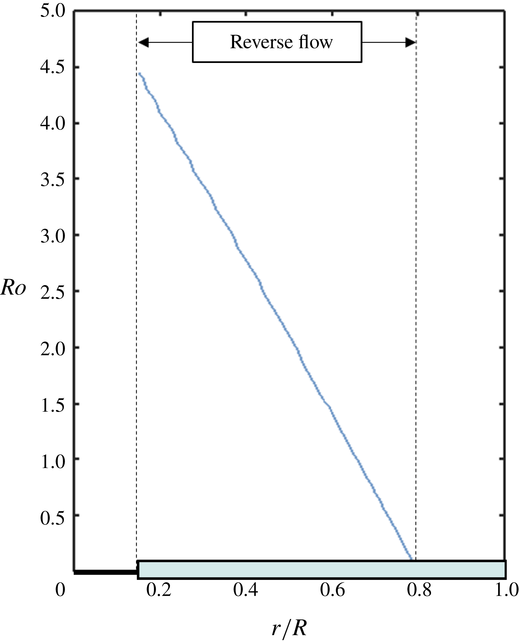
Distribution of reverse flow Rossby number (as defined by (1.2)) along the span of the wing for the baseline flight condition.

The simulations presented in this study are intended mirror a real rotor system, owned by the University of Maryland, that has been subject to considerable experimental investigation in past works (Berry & Chopra Reference Berry and Chopra2014; Trollinger et al.
Reference Trollinger, Wang and Chopra2017; Lind et al.
Reference Lind, Trollinger, Manar, Chopra and Jones2018). This rotor is outfitted with four untwisted rotor blades, each with a radius of 0.85 m, an aspect ratio of 10.63 and a NACA0012 airfoil cross-section. Table 1 details the flight condition that will serve as the baseline case for the remainder of the current work. At this condition, the extent of the reverse flow region is expected to be large, and the distribution of Rossby number along the blade span predicts a significant rotational component of the flow. Figure 3 shows the spanwise distribution of Rossby number for the baseline flight condition; the local Rossby number is
 $O(1)$
over a significant portion of the blade (
 $0.165<r/R<0.70$
) as it passes through reverse flow. The ability of Rossby number to predict vortex stabilization in reverse flow will be revisited at length in the results section.
As a final comment, the authors acknowledge that an articulated rotor does not represent the most fundamental model of a rotating wing in forward flight. A rotating wing is more typically modelled as a flat plate at a constant angle of attack, with flow separation along the span of the wing for its entire revolution, rather than the more complex case of an articulated rotor. The use of articulated rotor does, however, form an important link with previous works that concern the physics of the reverse flow region. In particular, Kirk & Jones (Reference Kirk and Jones2018) compared 2-D surging wing experiments at a constant angle of attack to the flow field of a spinning rotor and note significant differences in the evolution of the reverse flow vortex, but it remains unclear whether these differences were due to 3-D effects or articulation on the rotor. It can thus be seen a secondary goal of the current work to provide a link to these past assessments of 3-D effects in forward flight by clarifying the role of articulation in reverse flow.
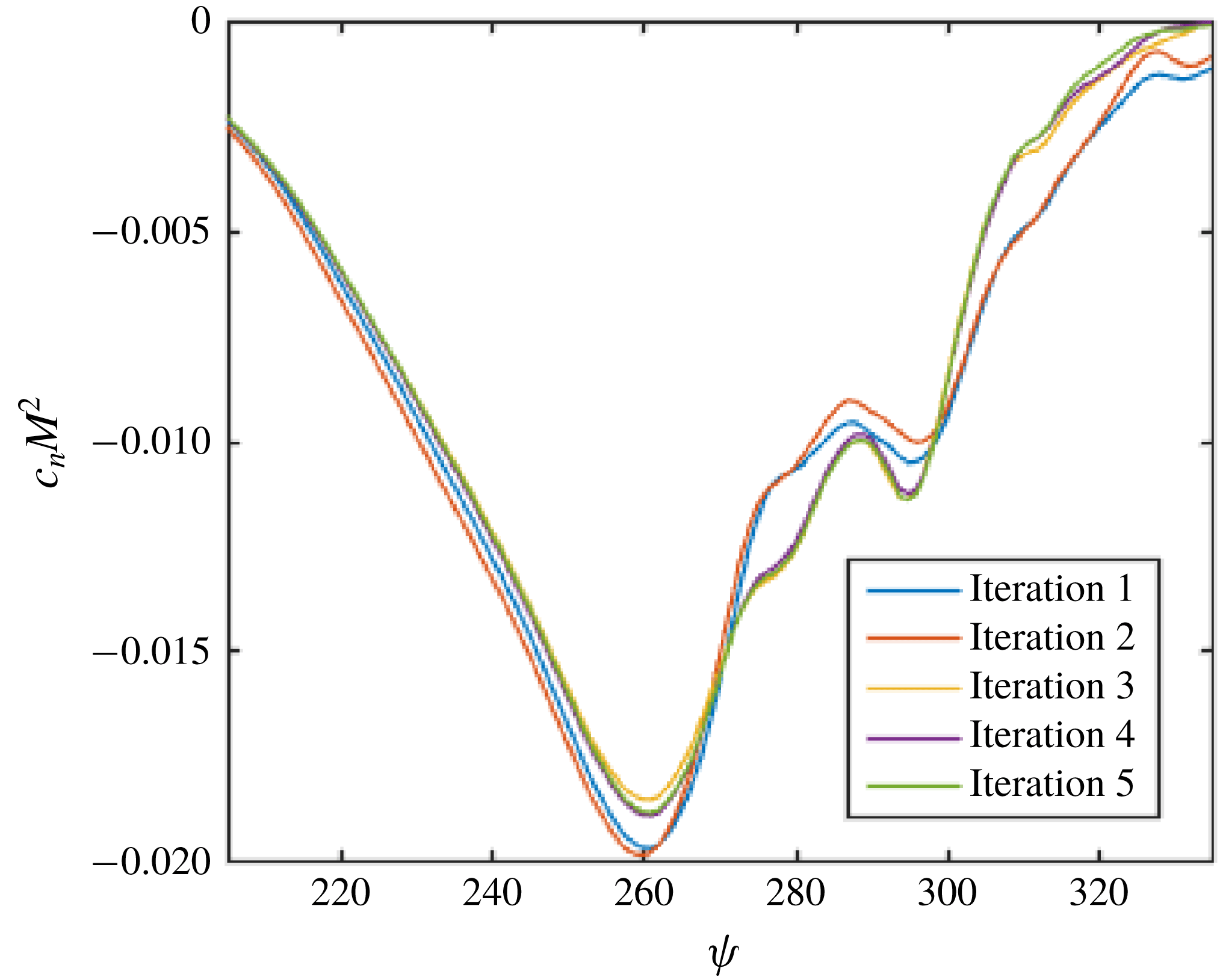
Predictions of section normal force coefficient at the
 $r/R=0.30$
radius position over successive iterations of the CFD-CSD coupling procedure.

2.2 Computational methods
High-fidelity numerical simulations were performed by solving the unsteady Reynolds-averaged Navier–Stokes equations on a volumetric mesh. The governing equations were discretized based on a finite volume method using a Hamiltonian/Strand flow solver (HAMSTR) designed for rotating wing applications. HAMSTR assumes compressible, viscous, and fully turbulent flow and achieves closure with the Spalart–Allmaras turbulence model. The flow field was computed every one degree of rotor revolution, and a second-order backward time-stepping procedure was used to advance the solution. A fifth-order weighted essentially non-oscillatory scheme was used for spatial reconstruction, while Roe’s approximate Riemann solver was used to compute the inviscid fluxes. Viscous fluxes were handled with second-order central differencing. Flow field results from HAMSTR were coupled with PrasadUM, a structural dynamics solver based in Euler–Bernoulli beam theory, to properly predict the deflections experienced by each rotor blade throughout its revolution. Convergence of the computational fluid dynamics/computational structural dynamics procedure (CFD-CSD) was defined based upon the behaviour of the normal force (
 $c_{n}$
) at the
 $r/R=30\,\%$
radius position. Figure 4 shows trends in sectional normal force within the reverse flow region (
 $205^{\circ }\leqslant \unicode[STIX]{x1D713}\leqslant 335^{\circ }$
) over five successive iterations of the CFD-CSD coupling and reveals very little change following the third iteration.
The veracity of these simulations was discussed at length in regard to sectional normal force predictions by Wang et al. (Reference Wang, Jung, Baeder and Chopra2018); however, it is also important that one assesses the accuracy of these simulations based on the flow fields themselves. The CFD-CSD coupling procedure was thus rerun at a slightly different forward flight condition (
 $\unicode[STIX]{x1D707}=0.60$
,
 $\unicode[STIX]{x1D703}_{0}=10^{\circ }$
and
 $\unicode[STIX]{x1D6FA}=900~\text{RPM}$
) to allow for comparison with experimental flow field measurements taken by the authors on the same rotor system (Smith et al.
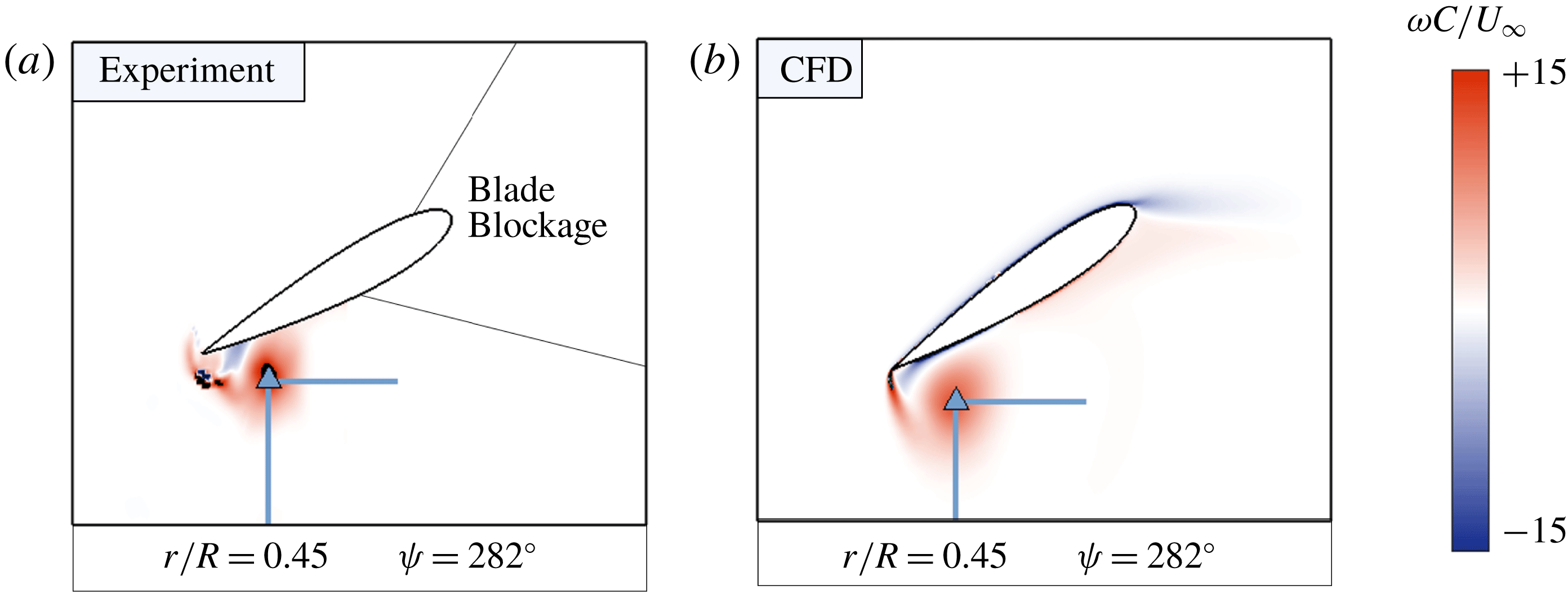
Reference Smith, Bauknecht, Wang, Lind and Jones2018). As an illustration of this comparison, figure 5 shows contours of the non-dimensional vorticity field at
 $r/R=0.45$
taken from phase-averaged experimental measurements (a) and CFD simulation (b). This flow field snapshot corresponds to
 $\unicode[STIX]{x1D713}=282^{\circ }$
, well after the
 $r/R=0.45$
radius position has transitioned into reverse flow. Although the experimental flow fields are missing vorticity due to blade blockage and reflections, a sharp-edge vortex is clearly visible, and appears to be of similar size, in both the experimental and computational flow fields.
Qualitative comparison of the sharp-edge vortex from experimental measurements (a) and CFD simulation (b) at a representative azimuth (
 $\unicode[STIX]{x1D713}=282^{\circ }$
) for
 $r/R=0.45$
.

This sharp-edge vortex was the subject of a more quantitative study intended to further explore the veracity of the CFD simulations. As a way of comparing the temporal evolution of the sharp-edge vortex, values of vortex strength were extracted from the experimental and computational flow fields. The vortex strength calculation procedure consisted of three main steps and was identical for both experimental and numerical data. First, a vortex centre was identified using the
 $\unicode[STIX]{x1D6E4}_{1}$
criterion of (Graftieaux, Michard & Grosjean Reference Graftieaux, Michard and Grosjean2001). The
 $\unicode[STIX]{x1D6E4}_{1}$
criterion physically represents a measure of the local rotation surrounding a certain point in the flow field, and is defined according to
 $$\begin{eqnarray}\unicode[STIX]{x1D6E4}_{1}=\frac{1}{A}\int _{A}\sin \unicode[STIX]{x1D719}\,\text{d}A,\end{eqnarray}$$
where
 $A$
is an area of integration, and
 $\unicode[STIX]{x1D719}$
is the angle between the position and velocity vectors at a given point. Vortex centres were identified based on local maxima in the
 $\unicode[STIX]{x1D6E4}_{1}$
criterion and are denoted by blue triangles in figure 5.
Next, two lines are drawn in each flow field, one line extending below the vortex centre and a second line extending to the right of the vortex centre. Examples of these lines are sketched in green in figure 5. The velocity field along these two lines are then fit to the Lamb–Oseen model of a rotational vortex, defined by
 $$\begin{eqnarray}u_{\unicode[STIX]{x1D703}}=\frac{\unicode[STIX]{x1D6E4}}{2\unicode[STIX]{x03C0}x}(1-\text{e}^{x^{2}/x_{c}^{2}}),\end{eqnarray}$$
where
 $u_{\unicode[STIX]{x1D703}}$
corresponds to the velocity component perpendicular to each line;
 $\unicode[STIX]{x1D6E4}$
corresponds to the strength of the vortex;
 $x$
corresponds to the distance of each point from the vortex centre; and
 $x_{c}$
is a vortex core radius that results from the fit. For a given experimental or computational flow field, the two values of
 $\unicode[STIX]{x1D6E4}_{1}$
produced by (2.4) (one for each line) are then averaged to arrive at a final value of the vortex strength. The purpose of employing this method of finding the vortex strength, as opposed to more conventional control volume methods, is that it avoids using data very near the surface of the wing, which are unavailable in the experimental measurements due to blade reflections.
Comparison of vortex strength from experimental measurements (left) and CFD simulation (right) for the
 $r/R=0.45$
radial station at a slightly altered flight condition (
 $\unicode[STIX]{x1D707}=0.60$
,
 $\unicode[STIX]{x1D703}_{0}=10^{\circ }$
,
 $\unicode[STIX]{x1D6FA}=900~\text{RPM}$
).

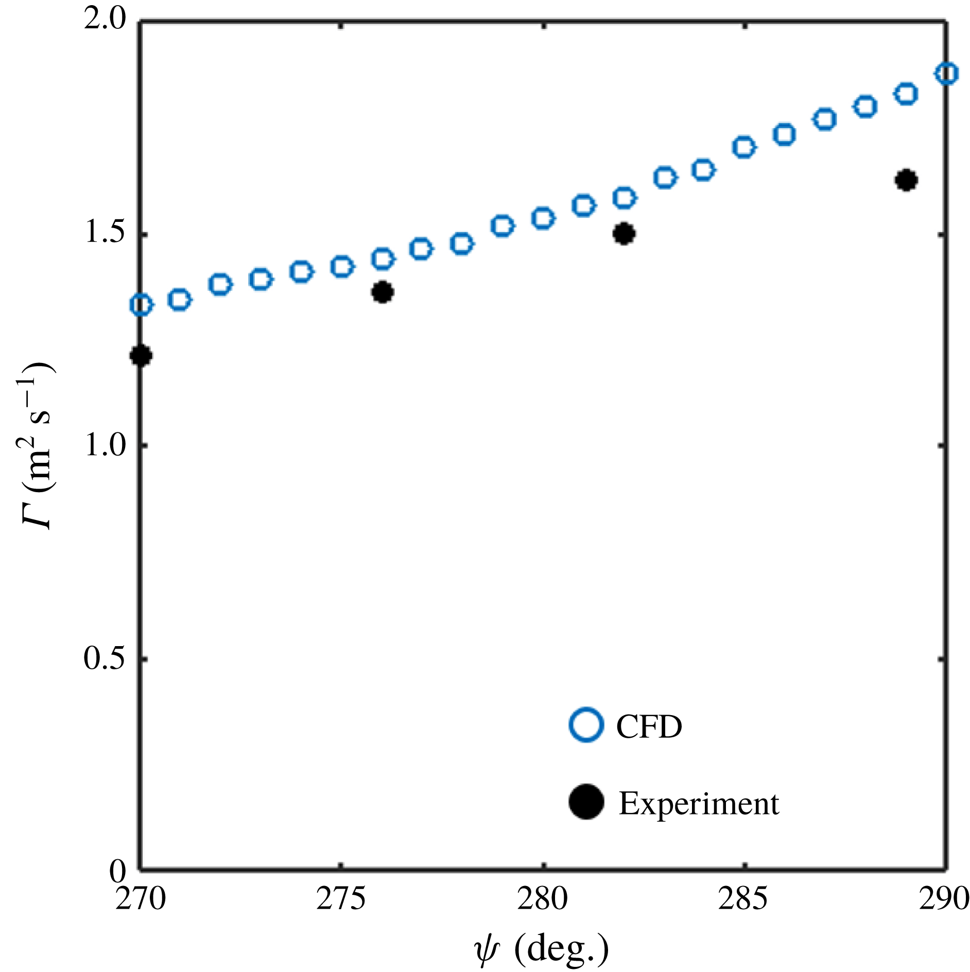
Figure 6 provides a comparison of the vortex strength, as computed using the Lamb–Oseen vortex fit, between the experimental measurements (black dots) and CFD simulations (blue dots) at the
 $r/R=0.45$
radial position as it passes through the reverse flow region. The computations show a very similar temporal evolution of the sharp-edge vortex. The slight over-prediction in the CFD can be attributed to a small inaccuracy in the CFD-CSD coupling procedure; the numerical results tend to over-estimate the longitudinal cyclic control angle (
 $\unicode[STIX]{x1D703}_{1s}$
), leading to a larger pitch angle in the computational flow fields. Overall, however, the values of vortex strength are comparable between the CFD and experimental measurements, and lend confidence to HAMSTR’s ability to predict sharp-edge vortex formation on rotating wings, despite lacking a more detailed turbulence model. Additional details regarding HAMSTR, its application to three-dimensional problems, and its convergence properties can be found in the works of Jung, Govindarajan & Baeder (Reference Jung, Govindarajan and Baeder2016, Reference Jung, Govindarajan and Baeder2017).
3 Results
This section aims to quantify the role of 3-D vortex dynamics in the reverse flow region of a rotating wing. In § 3.1, the flow morphology of the baseline condition will be presented as a way of introducing the relevant flow structures and gradients that arise along the wing span. In § 3.2, a vorticity transport analysis will be performed to quantify the relative contribution of 3-D effects to the evolution of vortical structures near the wing surface. Finally, § 3.3 will assess whether the Rossby number, as defined in (1.2), is an accurate prediction of the importance of Coriolis forces, and rotation in general, on the evolution of vortices in reverse flow.
3.1 Flow morphology
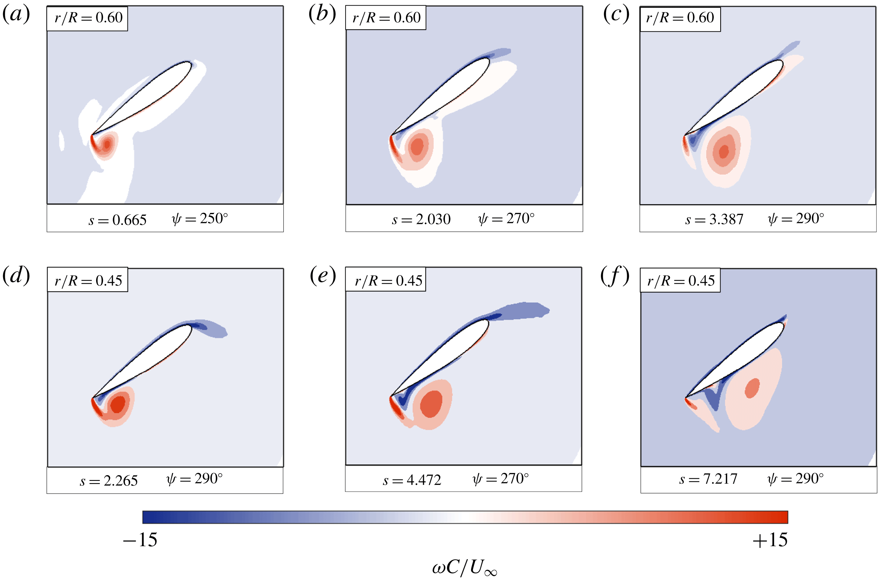
Contours of spanwise vorticity (
 $\unicode[STIX]{x1D714}_{z}$
) for wing radial locations of
 $r/R=0.60$
(a–c) and
 $r/R=0.45$
(d–f) at the baseline forward flight condition.

Figure 7 shows blade-element snapshots of one rotor blade at the baseline flight condition. In each panel, the local flow field is plotted in a non-inertial, rotating reference frame that travels with the blade element throughout its revolution. Non-dimensional chordwise distance is plotted on the
 $x$
-axis, non-dimensional vertical distance is plotted on the
 $y$
-axis and the rotor blade is overlain with contours of non-dimensional spanwise vorticity (
 $\unicode[STIX]{x1D714}c/U_{\infty }$
). Flow field snapshots are provided for the blade’s passage through the reverse flow region, and thus the local free-stream velocity is travelling from left to right. Convective time
 $s$
, or the number of semi-chords travelled by a blade element in reverse flow, is also denoted for each flow field snapshot. A mathematical definition of convective time is provided in (3.1), where
 $t_{i}$
and
 $t_{f}$
represent the time at which the blade element enters and leaves reverse flow, respectively:
 $$\begin{eqnarray}s=\frac{2}{c}\int _{t_{i}}^{t_{f}}U_{T}(t)\,\text{d}t.\end{eqnarray}$$
The blade element at
 $r/R=0.60$
(figure 7
a–c) illustrates the basic stages of vortex formation in the reverse flow region. Shortly after flow reversal, flow separates about the sharp edge of the wing and rolls up into a coherent vortex (
 $\unicode[STIX]{x1D713}=250^{\circ }$
). The separated shear layer feeds the vortex while it grows and convects. Closer to the exit of reverse flow, the vortex begins to lift off the surface of the wing, and a region of opposite-signed (blue) vorticity develops on the surface beneath it (
 $\unicode[STIX]{x1D713}=290^{\circ }$
). The blade element at
 $r/R=0.45$
(figure 7
d–f) exhibits very similar stages of vortex formation. Flow separates, rolls up into a coherent vortex and is continuously fed by a shear layer emanating from the sharp edge of the blade. The main difference is that at a given time, the vortex
 $r/R=0.45$
appears more ‘developed’ compared to the vortex at
 $r/R=0.60$
. That is, the vortex at
 $r/R=0.45$
is larger and contains a higher magnitude of vorticity for
 $250^{\circ }<\unicode[STIX]{x1D713}<290^{\circ }$
; it has also convected further and grown more diffuse by
 $\unicode[STIX]{x1D713}=290^{\circ }$
. The different vortex evolutions are likely due to the local free-stream values experienced by the two blade elements, as inboard regions see a higher local free stream than outboard elements in the reverse flow region.
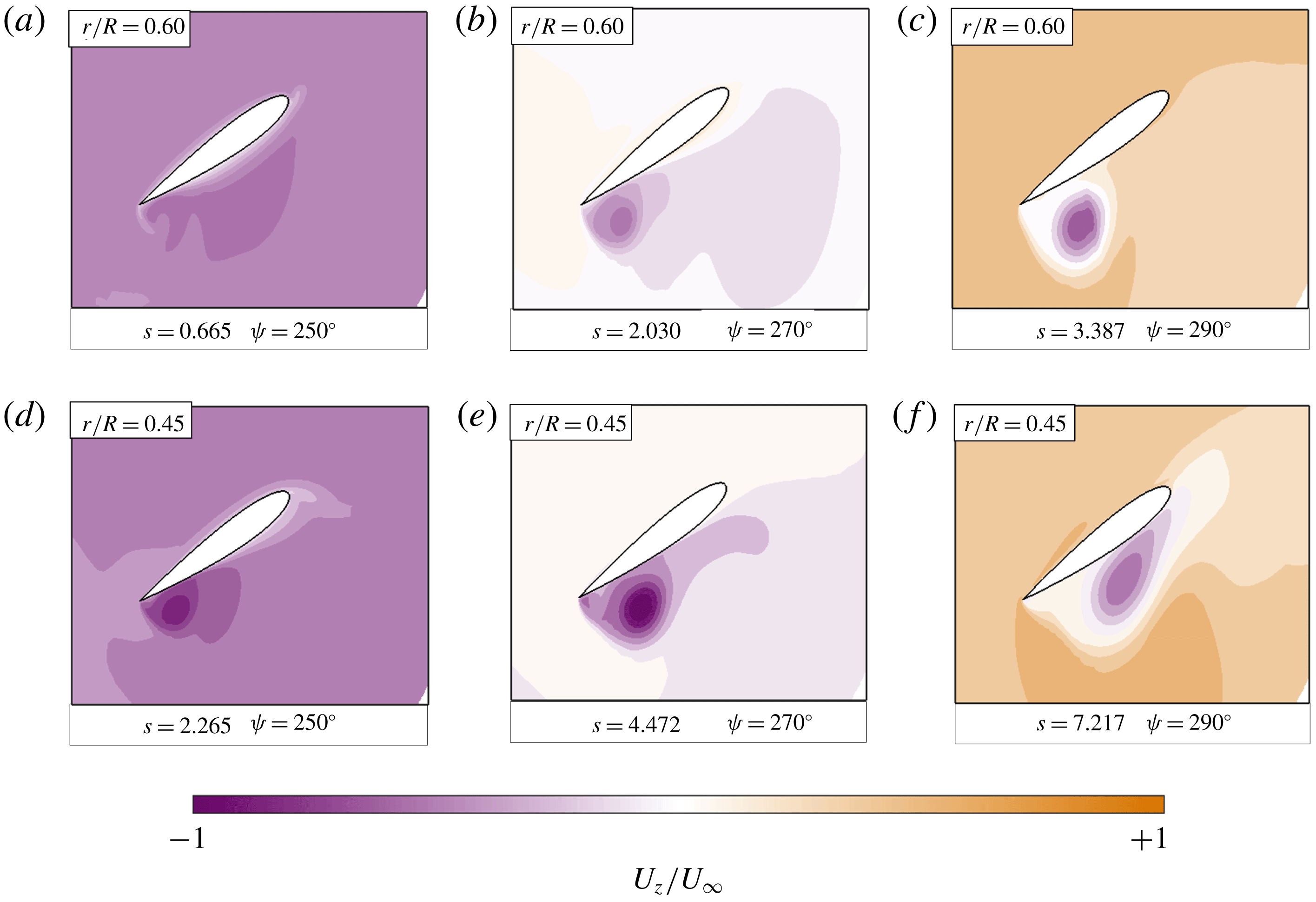
Contours of spanwise flow (
 $u_{z}$
) for wing positions of
 $r/R=0.60$
(a–c) and
 $r/R=0.45$
(d–f) at the baseline forward flight condition.

Figure 8 shows contours of spanwise flow, or the flow component in the
 $z$
-direction, for the same two blade-element positions discussed above. The spanwise flow field is dominated by a ‘background’ spanwise flow that alternates from tip-to-root (purple) for
 $\unicode[STIX]{x1D713}<270^{\circ }$
to root-to-tip (orange) for
 $\unicode[STIX]{x1D713}>270^{\circ }$
. This background spanwise flow is a result of the blade continuously reorienting itself relative to the forward flight velocity and is expected for a rotating wing in forward flight. Figure 8 also shows a region of tip-to-root spanwise flow near the vortex core. The amount of core flow grows in time and increases in magnitude as one moves from the
 $r/R=0.60$
position to the
 $r/R=0.45$
position.
Figures 7 and 8 illustrate the main aerodynamic characteristics of a rotating wing in reverse flow: the formation of a large vortex in the reverse flow region and the development of gradients in both vorticity and spanwise flow along the blade span. Although 3-D flow effects are evident, these figures alone do not indicate whether the presence of rotation has a significant effect on the evolution of the reverse flow vortex. The next section will explicitly address the role of 3-D flow physics by quantifying each term in the vorticity transport equation.
3.2 Vorticity transport analysis
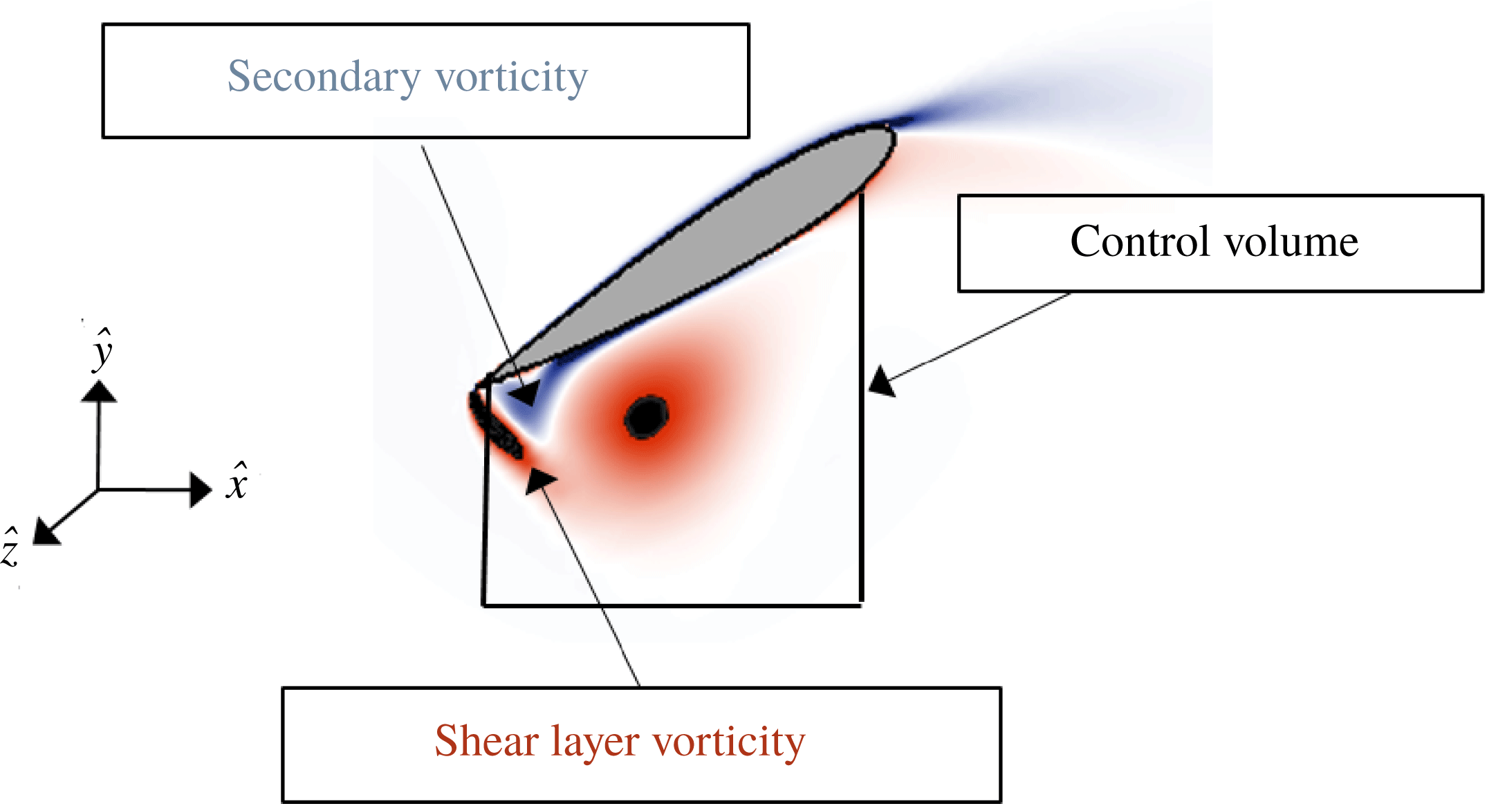
The purpose of this section is to quantify the relative importance of 2-D and 3-D vortex dynamics on a rotating wing in forward flight. This goal can be achieved by performing a control volume analysis over a blade’s passage through the reverse flow region. Illustrated in figure 9, a 2-D control volume was defined such that the upper surface of the volume coincided with the suction surface of the wing over a region that included the reverse flow vortex for much of the blade’s passage. This specific control volume was chosen as a way of isolating the vorticity transport mechanisms relevant to the sharp-edge vortex in reverse flow. If the control volume in figure 9 extended further downstream, for instance, it could become difficult to differentiate whether a change in circulation is due to positive vorticity entering the sharp-edge shear layer, or negative vorticity leaving the trailing wake at the blunt edge.
The total rate of change of circulation within this control volume is governed according to the integral form of the vorticity transport equation, given by
 $$\begin{eqnarray}\frac{\unicode[STIX]{x2202}\unicode[STIX]{x1D6E4}}{\unicode[STIX]{x2202}t}=-\int _{C}\unicode[STIX]{x1D714}_{z}(\boldsymbol{u}_{2D}\boldsymbol{\cdot }\hat{\boldsymbol{n}})\,\text{d}C+\int _{C}u_{z}(\unicode[STIX]{x1D74E}_{2D}\boldsymbol{\cdot }\hat{\boldsymbol{n}})\,\text{d}C+\unicode[STIX]{x1D708}\int _{C}\frac{\unicode[STIX]{x2202}\unicode[STIX]{x1D714}_{z}}{\unicode[STIX]{x2202}n}\,\text{d}C-\int _{C}(2\unicode[STIX]{x1D734}\times \boldsymbol{u})\boldsymbol{\cdot }\,\text{d}\boldsymbol{l},\end{eqnarray}$$
where
 $\boldsymbol{u}_{2D}$
is a vector representing the in-plane components of velocity (i.e.
 $\boldsymbol{u}_{2D}=u_{x}\hat{x}+u_{y}{\hat{y}}$
);
 $\unicode[STIX]{x1D74E}_{2D}$
represents the in-plane components of the vorticity vector (i.e.
 $\unicode[STIX]{x1D74E}_{2D}=\unicode[STIX]{x1D714}_{x}\hat{x}+\unicode[STIX]{x1D714}_{y}{\hat{y}}$
);
 $\hat{\boldsymbol{n}}$
represents a vector normal to the edges of the control volume; and
 $\boldsymbol{d}\boldsymbol{l}$
represents a vector tangent to the edges of the control volume. The vectors
 $\boldsymbol{u}$
and
 $\unicode[STIX]{x1D74E}$
correspond to the complete, 3-D velocity and vorticity vectors in a reference frame rotating with the wing. Note that the description of vorticity transport provided in (3.2) is similar to the form given by Eldredge & Jones (Reference Eldredge and Jones2019).
An advantage of (3.2) is that each term can be easily related to a physical mechanism present in the flow. From left to right, the terms in (3.2) correspond to the time rate of change of circulation, the in-plane (or 2-D) convection of vorticity, the tilting of vorticity, the viscous generation (or diffusion) of vorticity and transport due to Coriolis forces. Because of the high volumetric resolution of CFD, the contour integrals in (3.2) can be numerically evaluated along the selected control volume, and when compared to one another, illustrate the interplay between 2-D and 3-D transport mechanisms in reverse flow.
Control volume emanating from the lower surface of the wing at
 $r/R=0.45$
. The control volume has area
 $S$
, and its boundaries are denoted by the contour
 $C$
.

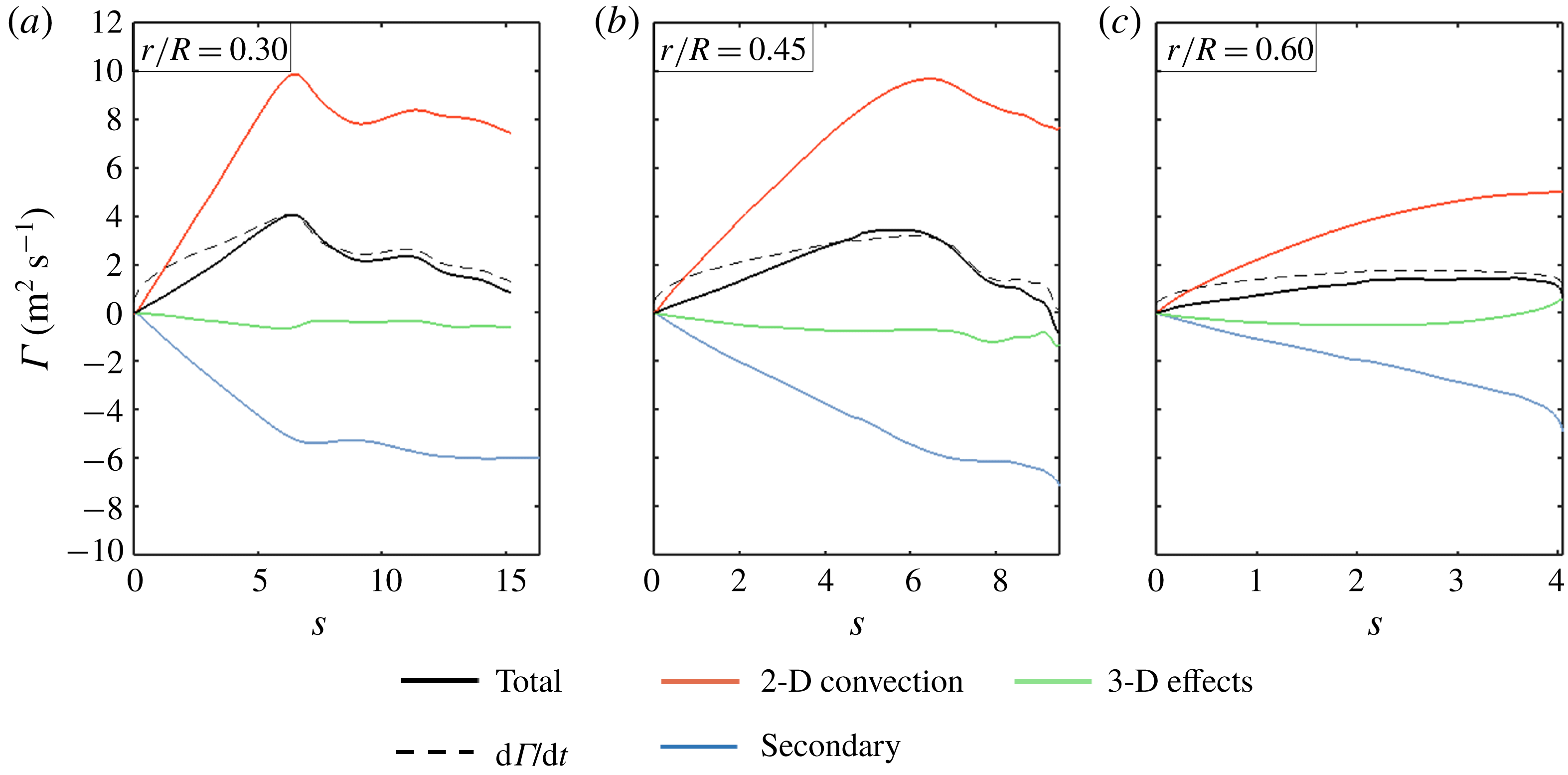
Figure 10 plots the contribution of each physical flow mechanism to the total circulation within the control volume at various radial stations throughout the reverse flow region. In each subfigure, convective time (i.e. the number of semi-chords travelled by each rotor blade element in reverse flow) is plotted on the
 $x$
-axis, and the contribution of each flow mechanism is plotted on the
 $y$
-axis. A summation of these contributions is represented by the solid black line, while a reference value for circulation, evaluated by taking the line integral of velocity, is plotted with the dashed black line. The solid and dashed black lines do not perfectly overlap; this is attributed to neglecting turbulent stresses within the control volume and only evaluating the viscous term along the blade surface in (3.2).
The vorticity contributions at
 $r/R=0.30$
(a) illustrate the role of each transport mechanism in reverse flow. The 2-D convection term (red line) adds significant positive circulation to the control volume as the shear layer feeds the reverse flow vortex. An opposite-signed vorticity (blue line), a result of the high-magnitude gradients that arise from enforcing the no-slip condition along the suction surface of the blade, follows the same basic trend over time. The 3-D effects term (green line) is a combination of vortex tilting and Coriolis forces; it maintains a very small magnitude throughout the evolution of the reverse flow vortex. This process, wherein the total circulation is dominated by shear layer vorticity and secondary vorticity, is also exhibited at
 $r/R=0.45$
(b) and
 $r/R=0.60$
(c).
The contribution of 2-D convection, secondary vorticity and 3-D vortex dynamics to the strength of the reverse flow vortex at (a)
 $r/R=0.30$
, (b)
 $r/R=0.45$
and (c)
 $r/R=0.60$
.

3.3 Discussion
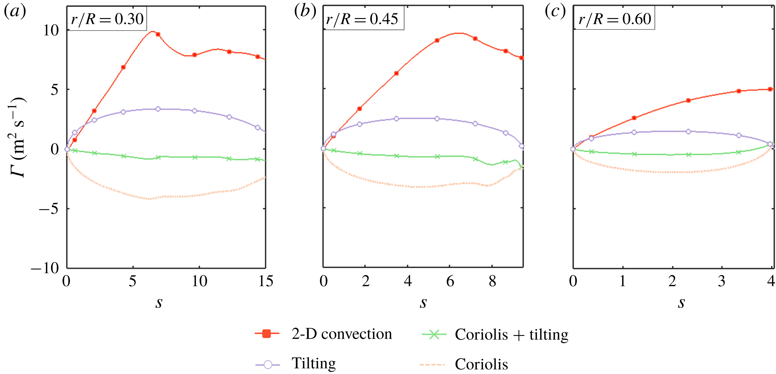
At this point, the original goals for this work as proposed in § 1 are revisited. The first goal was to determine whether or not a modified expression for the local Rossby number, stated explicitly in (1.2), could predict the relative magnitude of Coriolis forces in the reverse flow region. Figure 11 breaks down the 3-D effects term (i.e. the green line in figure 10) into its constituent components: the Coriolis effect (orange) and the vortex tilting effect (purple). At each radial station, the Coriolis term is approximately of the same order of magnitude as the 2-D convection term for much of the reverse flow region. This would suggest that the local ratio of inertial to Coriolis forces is approximately of
 $O(1)$
; the same order of magnitude was predicted in figure 3. One may conclude that the local Rossby number can reasonably predict the relative order of Coriolis forces in forward flight, just as it does in hover.
The contribution of vortex tilting and Coriolis forces to the total 3-D vortex dynamics at (a)
 $r/R=0.30$
, (b)
 $r/R=0.45$
and (c)
 $r/R=0.60$
. The 2-D convection is also represented as a reference.

The second goal was to determine if Coriolis forces are the deciding factor in vortex stability when a rotating wing enters forward flight. The notion of vortex ‘stability’ generally refers to a state of the flow in which the strength and position of a vortex are temporally invariant (Wong et al. Reference Wong, Kriegseis and Rival2013; Wojcik & Buchholz Reference Wojcik and Buchholz2014b ; Wong & Rival Reference Wong and Rival2015). In mathematical terms, this state corresponds to a constant vortex strength in time, or
 $$\begin{eqnarray}\frac{\text{d}\unicode[STIX]{x1D6E4}}{\text{d}t}=0,\end{eqnarray}$$
where
 $\unicode[STIX]{x1D6E4}$
is the circulation contained with the vortex. Since the vortex in reverse flow is continually fed by a shear layer at the sharp edge of the wing, the vorticity transport equation indicates that an alternate mechanism of the flow, namely diffusion, vortex tilting, or Coriolis forces, must act as a ‘sink’ of vorticity for the stability condition in (3.3) to hold. With this in mind, figure 11 is revisited to consider whether vorticity transport due to Coriolis forces acts to ‘drain’ vorticity from the vortex in reverse flow, and whether this transport of vorticity is enough to balance the action of the shear layer at the sharp edge. Again, each line in figure 11 represents the total circulation transported into the control volume (positive) and out of the control volume (negative) due to Coriolis forces, vortex tilting and 2-D convection. The green line corresponds to the sum of the Coriolis and tilting lines and is only included in this figure as a reference.
Figure 11 reveals that the Coriolis term contributes a net negative circulation to the control volume, meaning it effectively removes vorticity from the reverse flow vortex, and carries a similar magnitude to the convection of vorticity in the shear layer. This observation is consistent with the work of Jardin (Reference Jardin2017), where an artificial increase in the magnitude of the Coriolis term was found to stabilize, or at least reduce, the growth rate of a sharp-edge vortex on a rotating wing in hover. However, figure 11 also reveals an additional phenomenon not observed in hover; that is, the net transport due to Coriolis forces (orange) is nearly equal and opposite to the effect of vortex tilting (purple). The result is a cancelation of the Coriolis term with the vortex tilting term. The combined effect of vortex tilting and Coriolis forces is in turn an order of magnitude of lower than the 2-D convection of vorticity, and the net contribution of 3-D effects to the circulation of the reverse flow vortex is quite small. From this baseline case, the magnitude of Coriolis force does not appear to have a significant impact of vortex stability in reverse flow, despite the local Rossby number being of
 $O(1)$
.
Thus, there exists a discrepancy: in hover, a Rossby number of
 $O(1)$
generally corresponds to a stabilization of vortices, but in the reverse flow region, a Rossby number of
 $O(1)$
has little to no effect on the evolution of vortices. This discrepancy can be addressed by considering the direction of gradients in the reverse flow region. Consider an expression for the net effect of Coriolis forces on the reverse flow vortex, given by (3.4):
 $$\begin{eqnarray}-\int _{C}(2\unicode[STIX]{x1D734}\times \boldsymbol{u})\boldsymbol{\cdot }\,\text{d}\boldsymbol{l}=-\int _{C_{2}}\unicode[STIX]{x1D6FA}u_{z}\,\text{d}l.\end{eqnarray}$$
The purpose of (3.4) is to show that vorticity transport due to the streamwise Coriolis force is oriented with the negative of the spanwise flow direction, which is true in both hover and in forward flight. Keep in mind that
 $x$
corresponds to the wing chordwise direction,
 $y$
corresponds to the vertical,
 $z$
corresponds to the spanwise direction (with
 $+z$
pointing outboard) and
 $C_{2}$
corresponds to the bottom edge of the control volume sketched in figure 9. Likewise, the vorticity transport due to the spanwise Coriolis force (
 $-u_{x}\unicode[STIX]{x1D714}$
) disappears from the contour integral in (3.4) since our analysis is concerned only with the spanwise component; that is, its contour is defined with no component in the
 $\hat{z}$
direction.
Next, consider an expression for the spanwise convection of vorticity, given by (3.5). This expression is contained within the vortex tilting term provided in (3.2) and has been formally derived by Medina & Jones (Reference Medina and Jones2016):
 $$\begin{eqnarray}\int _{S}-u_{z}\frac{\unicode[STIX]{x2202}\unicode[STIX]{x1D714}_{z}}{\unicode[STIX]{x2202}z}\,\text{d}A.\end{eqnarray}$$
Equation (3.5) implies that the direction of spanwise convection depends on the local spanwise gradient in vorticity. In hover, the gradient in vorticity is oriented outboard, in the
 $+z$
direction. The spanwise convection term is thus aligned with the negative of the spanwise flow, just like the Coriolis term. In the reverse flow region, we saw in figure 7 that the spanwise gradient in vorticity is in fact oriented inboard, in the
 $-z$
direction. Thus, reverse flow sees the Coriolis and spanwise convection terms opposing one another due to the directional change in vorticity gradient. If these two terms are of a similar order of magnitude, as a Rossby number of
 $O(1)$
would imply, Coriolis and spanwise convection effects will tend to negate one another, leading to the situation observed in figures 10 and 11.
The preceding thought experiment implies that in reverse flow, a Rossby number of
 $O(1)$
is associated with equal and opposite Coriolis and vortex tilting terms, ultimately resulting in the negligible impact of 3-D effects on vortex evolution. This is a strong statement, and one that requires further evaluation. One way to validate this conclusion is by attempting to recreate the strength of vortices in reverse flow using only 2-D considerations. With this in mind, a simple vortex panel method was developed for the present work to simulate the 2-D physics of the flow at
 $r/R=0.30$
,
 $0.45$
and
 $0.60$
.
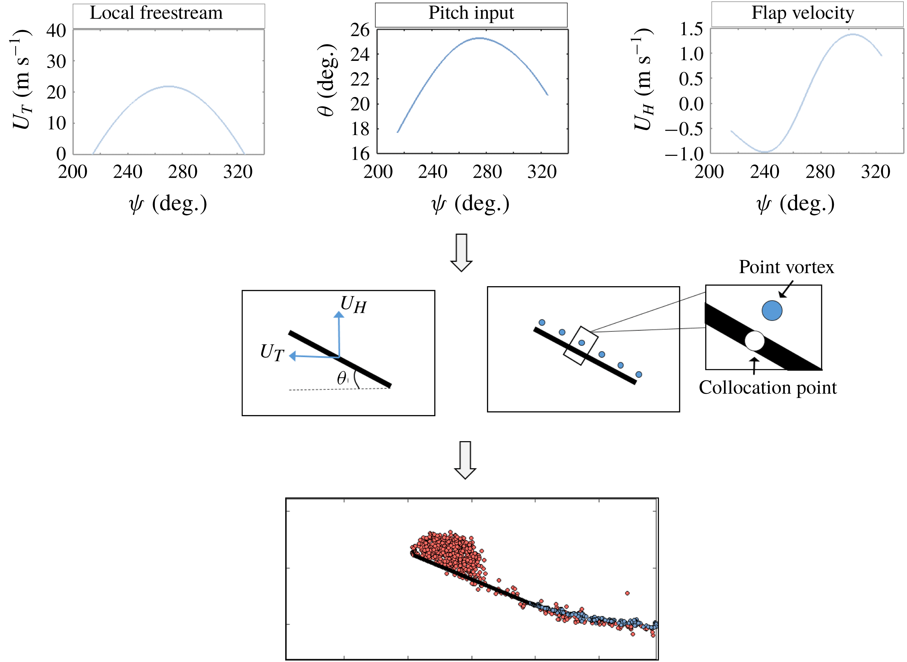
Figure 12 illustrates the operating principle of the unsteady panel method. The local unsteady free stream, flap deflection and angle of attack were extracted from the CFD data for a given radial station and discretized into an appropriate number of time steps (
 $\text{d}t=3c/(800U_{r,avg})$
). The rotor blade element is modelled as an infinitely thin flat plate composed of
 $N=64$
panels. Each panel is associated with a collocation point and a point vortex. At every time step, the strength of each point vortex is determined to enforce the no through-flow condition at the corresponding collocation point, and the Kutta condition at both the leading edge and the trailing edge. The vortices then convect with the local velocity field, and a new set of vortices is shed from the plate at the next time step. This procedure is similar to the low-order, inviscid vortex methods described by Spalart (Reference Spalart1988) and Manar & Jones (Reference Manar and Jones2019).
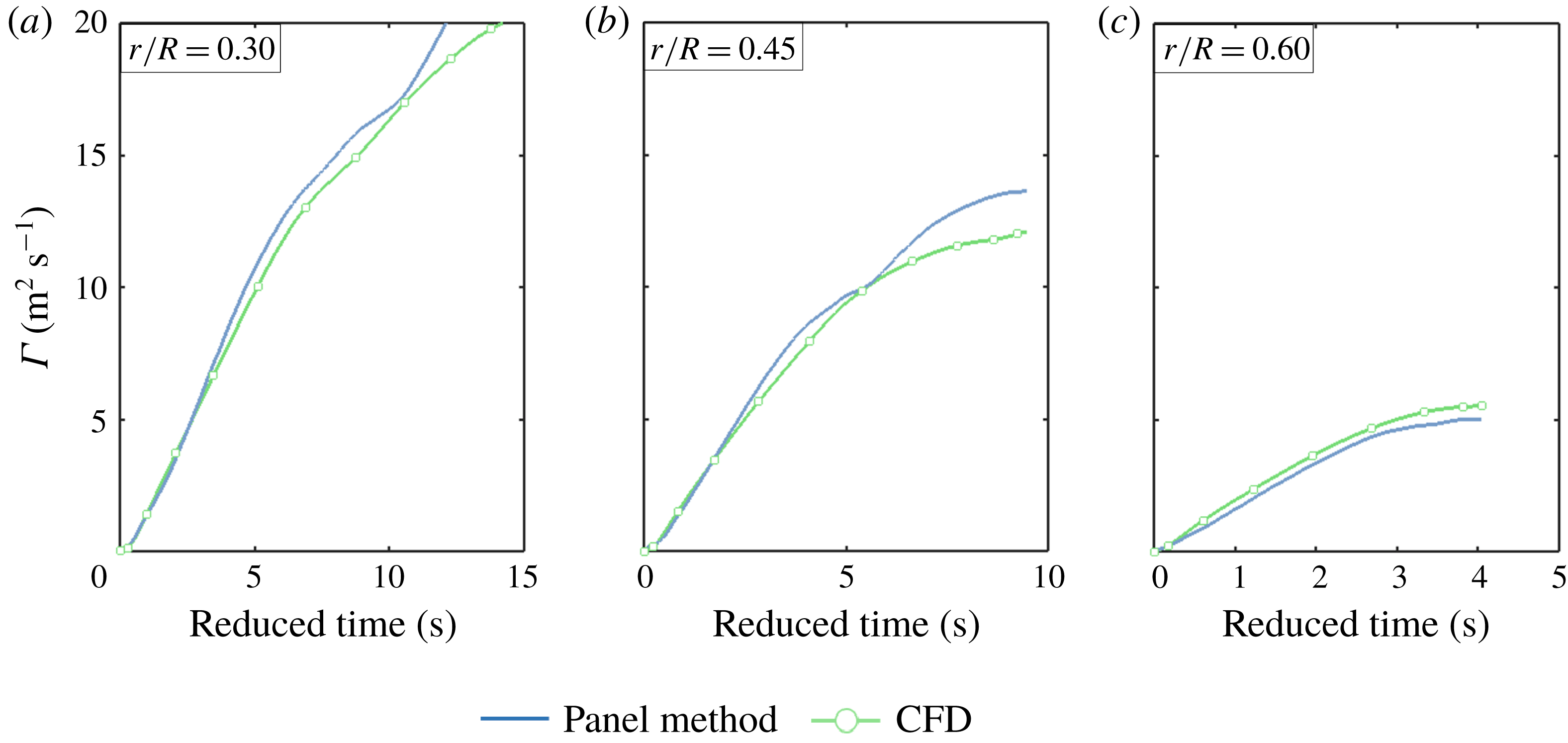
Operating principle for the unsteady vortex panel method. Wing motions are extracted from the CFD and used to solve for the strength of vortices shed from the wing.

Comparison in circulation production between the CFD and panel method simulations for (a)
 $r/R=0.30$
, (b)
 $r/R=0.45$
and (c)
 $r/R=0.60$
.

Figure 13 plots the total circulation produced at the leading edge of the wing for the panel method (solid blue line) and the CFD simulations (solid green line, with white circles) at three representative radial stations. Again, reduced time is plotted on the
 $x$
-axis and circulation is plotted on the
 $y$
-axis. Total circulation in the CFD simulations was calculated by integrating the flux of vorticity that arises from the shear layer at the sharp edge, while total circulation in the panel method was determined by simply summing the strength of each point vortex shed from the leading edge collocation point. Figure 13 shows good agreement between the low-order panel method and high-fidelity CFD results at
 $r/R=0.30$
,
 $r/R=0.45$
and
 $r/R=0.60$
. Each radial station saw a significant magnitude of Coriolis forces in the CFD (see figure 11), but vorticity production is nonetheless recreated by only considering the 2-D physics of the flow field in figure 13.
This agreement is an important observation in understanding the role of 3-D vortex dynamics in reverse flow. The preceding discussion has argued that the combined effect of vortex tilting and Coriolis forces is small in reverse flow if
 $Ro=O(1)$
; the reverse flow vortex is instead believed to be dominated by 2-D mechanisms of vorticity generation and convection. The unsteady panel method described above includes only these 2-D flow mechanisms and neglects the tilting and Coriolis terms in (3.2), but it is nonetheless able to reasonably predict the total circulation generated at the sharp edge of the wing in reverse flow. The results of figure 13 thus support the notion that 3-D vortex dynamics has a small impact on vorticity transport in reverse flow, a phenomenon explained here by the cancellation of Coriolis and vortex tilting effects when
 $Ro=O(1)$
.
As a final note, it is worth mentioning that figures 10, 11 and 13 are very much in conversation with the reverse flow experiments performed by Kirk & Jones (Reference Kirk and Jones2018). In this past work, the authors attempted to model the unsteady free stream seen in reverse flow with a pure surging wing at constant angle of attack (
 $\unicode[STIX]{x1D6FC}=25^{\circ }$
). The experiments were intended to replicate the flow field of a rotor blade element at
 $r/R=0.40$
passing through reverse flow over a range of advance ratios (
 $0.60<\unicode[STIX]{x1D707}<0.90$
). Kirk and Jones compared their results to the articulated rotor measurements of Lind et al. (Reference Lind, Trollinger, Manar, Chopra and Jones2018) and noted a significant difference in the stability of the reverse flow vortex between the surging and rotating cases, an observation originally attributed to the effects of rotary motion. It was theorized that the understanding of 3-D physics on a rotating wing in hover, where spanwise convection, vortex tilting and Coriolis effects combine to stabilize vortices formed at a sharp edge, may also be applicable to the reverse flow region of a rotary wing in forward flight.
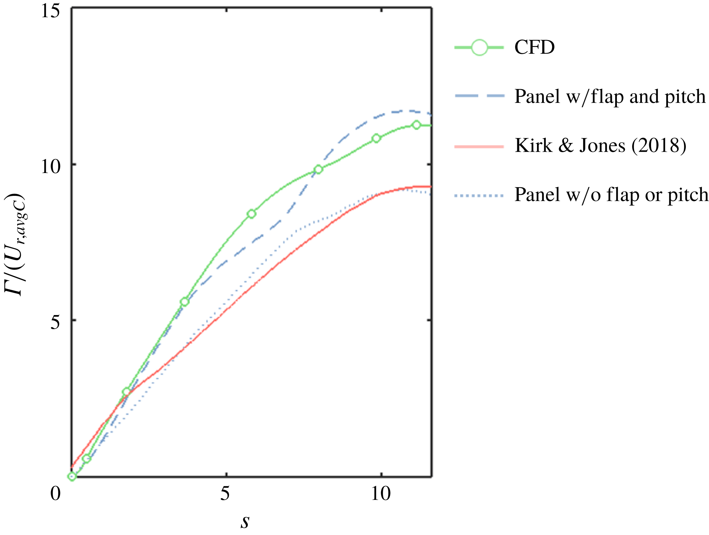
The effect of dynamic pitching and flapping on the circulation production of a blade element at
 $r/R=0.40$
for
 $\unicode[STIX]{x1D707}=0.80$
. The results of Kirk & Jones (Reference Kirk and Jones2018), which were performed with an unsteady free stream but no dynamic pitching or flapping, are included as a reference.

The current work argues that such a discrepancy is unlikely to result from rotation. Instead, it is believed that the discrepancy is more likely due to the presence of dynamic pitching and flapping on the articulated rotor tested by Lind et al. (Reference Lind, Trollinger, Manar, Chopra and Jones2018). Figure 14 attempts to isolate the role of blade pitching and flapping, motions inherent to an articulated rotor in forward flight, on circulation production in the reverse flow region. The results of Kirk & Jones (Reference Kirk and Jones2018) were analysed to extract values for the production of circulation at the sharp edge of the wing. These values are plotted as a solid red line and represent a wing in pure surge at constant angle of attack. The result of the current work’s CFD simulations are plotted in green (with white circles) and represent a four-bladed articulated rotor in forward flight. The 2-D panel method was run once to replicate the pitching and flapping kinematics of the CFD simulation at
 $r/R=0.40$
(dashed blue line), and once to replicate the simplified kinematics of Kirk and Jones (dotted blue line). Figure 14 shows that the rotating case (CFD) and surging case (Kirk and Jones) do indeed exhibit a discrepancy in circulation production at the sharp edge; however, this discrepancy is captured by the panel method with the simple addition of dynamic pitching and flapping. Rotation may still play a small role in circulation production, which can be generally seen in the deviations between the panel method and CFD, but figure 14 further illustrates that the magnitude of circulation production in reverse flow can be approximated from 2-D considerations alone.
4 Conclusions
The interplay between 2-D and 3-D vortex dynamics is highly complex on a rotating wing in forward flight. Especially in regions of reverse flow, it is unclear whether the conclusions associated with rotating wings in hover apply to the case of forward flight. In this work, high-fidelity numerical simulations were used to study the physics of reverse flow on an articulated rotor in forward flight. A vorticity transport analysis was conducted to assess whether Coriolis forces, a critical metric of vortex stability on rotating wings in hover, play a role in vortex evolution in the reverse flow region. The study focused on three radial stations (
 $0.30<r/R<0.60$
) at a large advance ratio (
 $\unicode[STIX]{x1D707}=0.80$
) and reached the following conclusions.
(i) An adjusted version of the Rossby number, where the characteristic velocity is set equal to the average reverse flow velocity, properly predicts the order of magnitude of Coriolis forces in the reverse flow region of a rotating wing in forward flight.
(ii) Despite the large magnitude of Coriolis forces, rotation in general was shown to play only a small part in the evolution of vortices in the reverse flow region. The vorticity transport analysis revealed that 2-D mechanisms, including shear vorticity and the viscous generation of secondary vorticity, far outweighed the magnitude of 3-D vortex dynamics at each of the radial stations considered here. In fact, a vortex panel method, developed using only the 2-D motions of the rotor blade, was able to model the growth rate of the reverse flow vortex at each of our radial stations and achieved close agreement with the high-fidelity results.
(iii) The small impact of 3-D physics is believed to be unique to the reverse flow region. It was shown that due to a change in the direction of spanwise vorticity gradients, the direction of vortex tilting is opposed to the direction of Coriolis effects in reverse flow. When these two effects are of a similar order of magnitude, as they are when
 $Ro=O(1)$
, spanwise convection effects tend to negate Coriolis effects. This process is quite different from the flow field on a rotating wing in hover.

Acknowledgements
This work was supported by the U.S. Army/Navy/NASA Vertical Lift Research Center of Excellence Cooperative Agreement with Mahendra Bhagwat serving as Program Manager and Technical Agent, grant number W911W6-17-2-0004.