1. Introduction
With the development of production automation and robot technology, industrial robots are widely used in processes such as palletizing, welding, material handling, and assembly. In order to meet the demands of complex work environments and strict production efficiency requirements, it is essential for robots to have optimal work paths. As a result, many scholars have conducted research on robot path optimization. Kim and Croft [Reference Kim and Croft1] proposed a method that found the maximum motion constraints based on the robot’s dynamic model, with the goal of minimizing the motion time at turning points in path optimization. This method improved motion accuracy and was computationally simple. Sun et al. [Reference Sun, Wang, Li, Qi and Zhang2] designed a path tracking controller based on adaptive dynamic programming. Specifically, it first selected an action dependent heuristic dynamic programming structure that met the requirements for tracking control. The control system designed in this paper achieved better tracking accuracy, faster convergence speed, and effectively reduced energy consumption during the control process. Wu et al. [Reference Wu, Yang, Huang, Ning and Zhang3] researched the dynamics and mechanical performance of industrial robots and established a trajectory optimization model based on convex optimization problems.They introduced convex optimization parameters to solve the inconsistency between constraint space and planning space, and proposed an adaptive optimization method to select optimal parameters. Finally, the problem was transformed into a second-order cone programming problem for solving. Howell et al. [Reference Howell, Cleac’h, Singh, Florence, Manchester and Sindhwani4] designed a dual-layer trajectory optimization framework that utilizes low-level optimization-based dynamics for trajectory optimization, enabling classical unconstrained solvers to optimize motion for more complex systems. However, this approach lacks convergence guarantees in finding solutions that satisfy dynamic representations. The method proposed by Schulman [Reference Schulman, Duan, Ho, Lee, Awwal, Bradlow, Pan, Patil, Goldberg and Abbeel5] used multiple sequential convex optimizations to approximate the non-convex optimization, thereby reducing the difficulty of solving the problem. In addition, to ensure that each subproblem is convex, some infeasible constraints were transformed into a penalty strategy. To maintain the quadratic form of the objective function, slack variables were added to the penalty terms, and constraints were imposed. Li et al. [Reference Li, Wang, Zhang, Feng, Lu and Zhai6] proposed a robotic motion optimization method based on Accelerated Gradient Descent and Directed-Mutagenesis Genetic Algorithm. By introducing a directed-mutagenesis mechanism and hierarchical weight updating, the approach overcame local optima and improved the success rate of collision-free path planning.Through mathematical modeling of the problem, the pseudospectral method can find a relatively accurate solution in a shorter computation time. In contrast, the genetic algorithm, when faced with complex nonlinear constraints, enlarges the search space to avoid local optima and explores more flexible solutions, but it typically requires more computational resources and time. Mukadam et al. [Reference Mukadam, Dong, Yan, Dellaert and Boots7] proposed the use of Gaussian processes to solve motion planning problems. By interpolating a small number of state points using Gaussian process, continuous trajectories based on gradient optimization algorithms could be obtained. Elgindy [Reference Elgindy8] proposed the Fourier Integral Pseudospectral method for nonlinear periodic control problems. The method transformed the control problem into a nonlinear programming problem using Fourier integration matrices for accurate integral approximation and was solved with numerical optimization. Its accuracy and efficiency were validated on two nonlinear control examples. Chen et al. [Reference Chen, Bai, Zhao, Wang, Yao and Chen9] introduced a two-phase pseudospectral convex control method for swarm systems. It used the Radau pseudospectral method to discretize and convexify goals and constraints, then applied a two-phase receding horizon approach to enhance speed and robustness. Simulations confirmed its effectiveness in collision avoidance and efficiency. Gao et al. [Reference Gao, Gong, Li, Guo, Fadda and Brandimarte10] presented an adaptive pseudospectral successive convex optimization algorithm for six-degrees-of-freedom powered descent, with applications in rocket landing and beyond. It combined global pseudospectral discretization with local linearization to convert the problem into a convex subproblem. A parameter-adaptive convexification algorithm adjusted the trust region size, while an adaptive grid method reduced local errors. Zhao et al. [Reference Zhao, Lin and Tomizuka11] proposed an optimal control method based on dynamic model to simultaneously solve path planning and trajectory planning problems. Experimental results show the feasibility of the proposed planning algorithm. Martín [Reference Moreno-Martín, Ros and Celaya12] combined the Legendre pseudospectral method with the Gauss pseudospectral method to optimize robot trajectories, ensuring that the velocity’s approximate polynomial was the time derivative of a merged polynomial. This approach made the trajectory more consistent with the system’s dynamics. Crain and Ulrich [Reference Crain and Ulrich13] used the Gauss pseudospectral method to solve the optimization problem of free-floating space robot paths. The goal was to minimize time, energy, and disturbances to the base position, and obtain the optimal path for the space robot from the initial pose to the target pose. Zhang et al. [Reference Zhang and Shi14] used quintic B-splines to generate trajectories, considering both kinematic and obstacle constraints. The Gilbert–Johnson–Keerthi collision detection algorithm was used to check for collisions. The constrained multi-objective PSO algorithm was employed to solve the time-jerk optimization problem.
Based on the relevant research mentioned above, it is found that using optimal control theory to transform the robot path optimization problem into a nonlinear programming problem can simplify the problem and improve computational efficiency. However, this method has not been widely tested in practical application environments, and current research is still in the simulation stage, with some distance from actual application. Therefore, further research on path optimization algorithms needs to be strengthened.
This research is based on the pseudospectral method to study the problem of robot path optimization. The algorithm can quickly plan a time-optimal trajectory in various complex work environments. The main contributions are as follows:
-
1. This paper presents, for the first time, a closed-loop adaptive weight adjustment pseudospectral method that employs the maximum joint acceleration as feedback to dynamically regulate the trajectory smoothness weight online during the optimization process, thereby improving work efficiency while effectively mitigating joint impact.
-
2. A comprehensive trajectory optimization model for a six-degree-of-freedom robotic manipulator is formulated, rigorously coupling kinematic and dynamic constraints along with boundary conditions to ensure both computational tractability and physical fidelity of the optimization problem.
-
3. A simplified collision detection method based on key separating axes is introduced, which significantly reduces the number of axes required for evaluation, thereby decreasing the computational complexity of three-dimensional (3D) collision detection and improving the efficiency of real-time collision avoidance.
2. Descripition of path optimization
2.1. System model
The robot path optimization problem involves targeting a specific performance index, meeting inherent state constraints, and determining the optimal or near-optimal path from the initial pose to the target pose. Therefore, the optimal running time of the robot in the feeding process can be regarded as an optimal control problem [Reference Teo, Li, Yu and Rehbock15], and the mathematical description of the optimal control problem is generally in the form of Bolza [Reference Peng, Jia-yuan and Xiu-yun16]. First, determine two functions,
 $t$
 $\rightarrow$
 $(x,t)$
and
 $t_f$
, and then realize the shortest time cost under the kinematics, dynamics, path, boundary, and collision constraints. The state and control in the path optimization involving the robot dynamics can be defined as:
 \begin{equation} x(t)=\begin{bmatrix} \theta (t) \\\dot {\theta } (t) \end{bmatrix},\quad u(t)=\tau (t) \end{equation}
where
 $t \in [t_0,t_f]$
,
 $\theta (t)=[\theta _1(t),\ldots ,\theta _6(t)]^T$
is the position vector of each joint of the robot,
 $\tau (t)=[\tau _1(t),\ldots ,\tau _n(t)]^T$
is the torque vector of each joint of the robot.
2.2. Adaptive objective function
The objective function in robot path optimization is typically expressed in a Bolza-type form:
 \begin{equation} J = t_f + \int _0^{t_f} \Psi [\textbf{x}(t), \textbf{u}(t)] \, \,{\rm d}t \end{equation}
In this work, both execution time and trajectory smoothness are considered. The optimization objective is defined as:
 \begin{equation} J = t_f + u \int _0^{t_f} \left ( \dddot {\theta }(t) \right )^2 B \, \,{\rm d}t \end{equation}
where
 $t_f$
is the total execution time,
 $\dddot {\theta }(t)$
is the third derivative of joint angles (jerk), and
 $u \geq 0$
is a weighting coefficient to balance time optimality and motion quality. The matrix
 $B$
is a penalty matrix that assigns greater weights to joints with larger gear ratios, and is defined as:
 \begin{equation} B_{ij} = \begin{cases} 0, & i \ne j \\[5pt] \dfrac {1}{A_{ij}^2}, & i = j \end{cases} \end{equation}
Here,
 $A$
is the gear transmission ratio matrix, and
 $A_{ij}$
represents the gear ratio of the
 $i$
-th joint.
In traditional approaches, the weight
 $u$
is typically a manually tuned constant. However, such a fixed coefficient cannot adapt to different trajectory profiles or task requirements, and may lead to excessively large joint accelerations, reducing feasibility or stability.
To address this, we propose an adaptive weight design based on trajectory acceleration characteristics, allowing
 $u$
to automatically adjust according to motion intensity. A normalized acceleration indicator
 $\eta$
is introduced to measure how close the trajectory is to the physical acceleration limits:
 \begin{equation} \eta = \max _j \left ( \frac {\max _t |\ddot {\theta }_j(t)|}{a_{\max ,j}} \right ) \end{equation}
where
 $a_{\max ,j}$
is the maximum allowable acceleration for joint
 $j$
. A larger
 $\eta$
indicates a more aggressive trajectory, potentially violating acceleration constraints.
To mitigate this, the weight
 $u$
is designed as an inverse function of
 $\eta$
:
 \begin{equation} u = \frac {1}{\max \left ( \ddot {\theta }_j(t) \right )}, \quad j = 1, 2, \ldots , n \end{equation}
To eliminate ambiguity, the definition is refined as:
 \begin{equation} u = \frac {1}{\max _j \max _t |\ddot {\theta }_j(t)|} \end{equation}
Equation (7) ensures that the largest absolute joint acceleration across all joints and the entire trajectory is used to control the trade-off. When acceleration becomes large,
 $u$
increases, enhancing the jerk penalty and producing a smoother trajectory. When acceleration is low,
 $u$
decreases to emphasize time minimization.
2.3. Dynamics constraints
Dynamic constraints are essential components of robot dynamics, and the kinetic equation is expressed as:
 \begin{equation} \begin{aligned} M(\theta )\ddot \theta +C(\theta ,\dot \theta )\dot \theta +G(\theta )=\tau \\J_mA\ddot \theta =\tau _d-A^{-1}\tau \end{aligned} \end{equation}
where
 $M(\theta )\in R^{n\times n}$
is the inertia matrix,
 $C(\theta ,\dot \theta )\dot \theta \in R^{n\times }$
is the Coriolis force and the centrifugal force terms,
 $G(\theta )\in R^{n\times 1}$
is the gravity matrix,
 $J_m$
is the inertia matrix of the motor,
 $A$
is the gear transmission ratio matrix,
 $J_m$
, and
 $A$
are the diagonal matrix.
 $\tau _d$
is the motor torque. For multi-joint robots, all terms in the dynamics equations are essentially nonlinear.
Make
 $x_1=\theta ,x_2=\dot \theta$
, dynamics constraints can be viewed as the state-space model with state
 $x=[x_1^T,x_2^T]^T$
and control
 $u=\tau$
:
 \begin{equation} \begin{cases}\dot x_1=x_2 \\\dot x_2=M(x_1)^{-1}[u-C(x_1,x_2)x_2-G(x_1)]\end{cases} \end{equation}
2.4. Path and boundary constraints
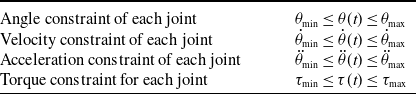
The path constraints in the robot path optimization problem are shown in Table I. According to Eq. (8),
 $\tau (t)$
can be expressed as:
 \begin{equation} \tau (t)=A\tau _d-AJ_mA\ddot \theta \tau (t) \end{equation}
The boundary conditions in the robot path optimization problem are shown in Table II. Among them,
 $\theta _0$
and
 $\theta _f$
are the initial and target joint positions of the robot, where
 $t_f^{\min}$
and
 $t_f^{\max}$
denote the lower and upper bounds of the runtime interval.
Path constraints.

Boundary constraints.

2.5. Collision constraints
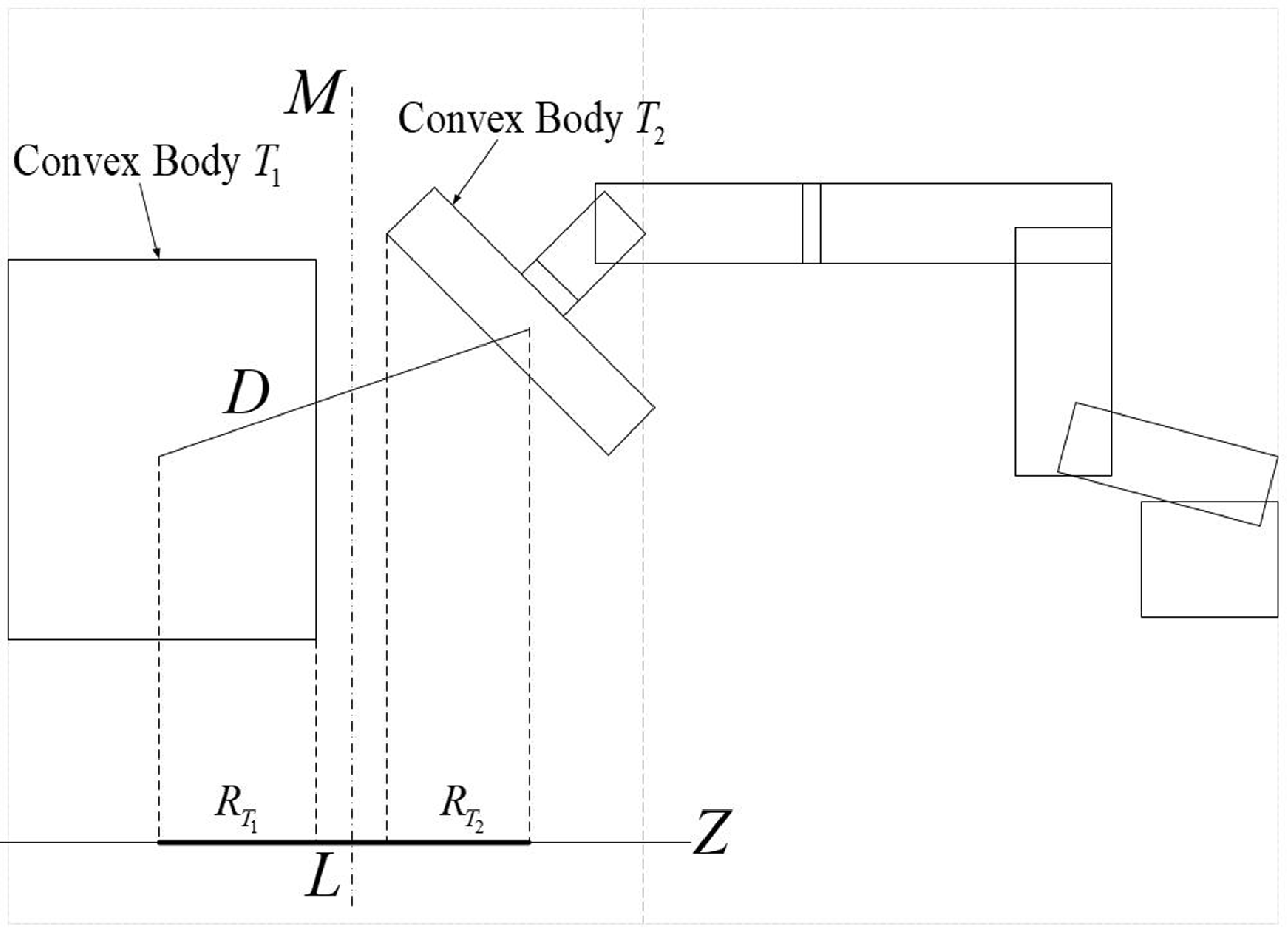
In order to quickly determine whether two objects collide, this paper utilizes oriented bounding boxes (OBBs) to construct geometric models of the robot and other components for collision detection calculations. OBBs are used to envelope the objects being detected, and their shape remains unchanged while allowing for real-time bounding [Reference Chang and Kim17]. The principal component analysis (PCA) method is a classic approach for computing OBB [Reference Prasanth and Shunmugam18]. The separating axis test algorithm, which is based on the separation hyperplane theorem in convex analysis, is used for collision detection specifically with OBB [Reference Kalantari19]. Its application in a 2D space is illustrated in Figure 1.
Detection of separation axes between bumps in 2D space.

As shown in the figure above,
 $M$
represents the separating hyperplane between convex bodies
 $T_1$
and
 $T_2$
. If the line
 $Z$
is perpendicular to the plane
 $M$
, it is called a separating axis. The line segment
 $D$
connects the centers of the convex bodies
 $T_1$
and
 $T_2$
. The projection of
 $D$
onto the
 $Z$
axis is denoted by
 $L$
.
 $R_{T_1}$
and
 $R_{T_2}$
are half of the projections of the convex bodies
 $T_1$
and
 $T_2$
onto the separating axis. Since the analysis and calculation of separating hyperplanes is complex, separating axes are commonly used as tools for intersection testing. The existence of a separating plane affects whether there is a separating axis or not, and the presence of a separating plane can be determined using Eq. (11).
 \begin{equation} R_{T_1}\lt R_{T_2} \end{equation}
The separation axis test for bounding boxes in 3D space is more complex than in 2D space. During the test, the two convex objects need to be projected onto 15 separating axes. These axes include the three coordinate axes of the bounding box of convex object
 $T_1$
, the three coordinate axes of the bounding box of convex object
 $T_2$
, and the nine axes generated by the cross product of the three coordinate axes of convex object
 $T_1$
with the three coordinate axes of convex object
 $T_2$
. If there is no separating plane between the two convex objects along any of these 15 separating axes, it can be determined that there is an intersection between the two convex objects.
Traditional Separating Axis Test algorithm requires the accumulation of 15 separating axes to complete the judgment, which is inefficient. In this paper, an effective collision detection algorithm in a static environment is used based on the approach proposed by Chang et al. [Reference Chang, Wang and Kim20], which only requires separation testing for 5 separating axes
 $\{A_1,B_1,C_{23},C_{32},C_{33}\}$
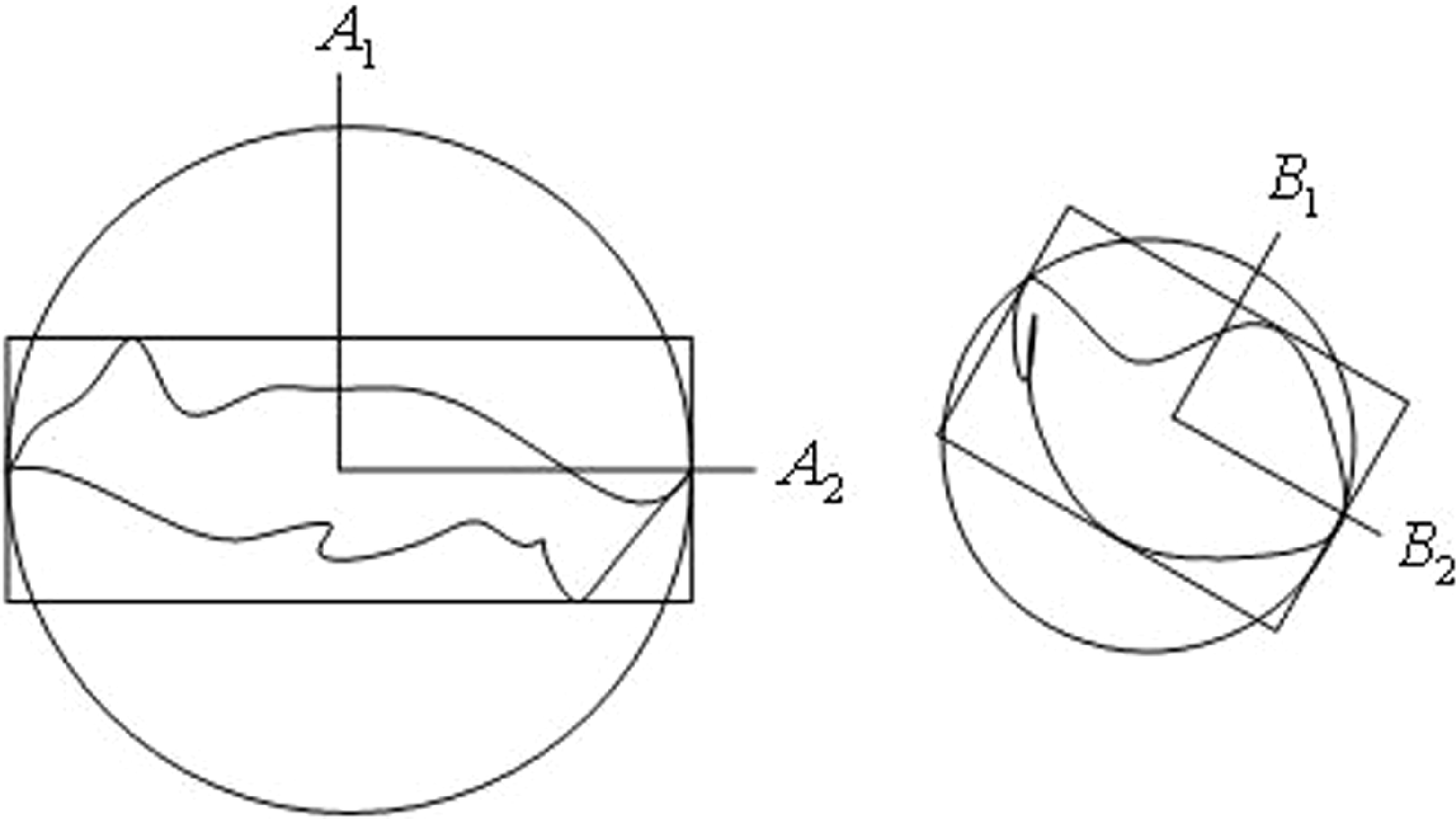
, thereby effectively improving the calculation efficiency. The algorithm consists of a directional bounding box tree with boundary spheres. First, the corresponding enclosed spheres are constructed using the directional bounding boxes of two convex bodies [Reference Gan and Dong21], as shown in Figure 2. Second, 15 separating axes
 $\{ A_1,A_2,A_3,B_1,B_2,B_3,C_{11},C_{12},C_{13},C_{21},C_{22},C_{23},C_{31},C_{32},C_{33}\}$
are defined, and axis
 $\{A_1,A_2,A_3\}$
is the coordinate axis of the first convex body directional bounding box. Its three edges are projected onto the corresponding coordinate axes, and the axis with the minimum length is defined as axis
 $\{A_1\}$
, and the axis with the maximum length is defined as axis
 $\{A_1\}$
. Axis
 $\{B_1,B_2,B_3\}$
is the coordinate axis of the second convex body directional bounding box. All axes are defined as mentioned above, and axis
 $\{C_{i,j}\}$
is the cross product of
 $\{A_i\}$
and
 $\{A_j\}$
,
 $i,j\in [1,3]$
.
Detection of separation axes between bumps in 2D space.

3. Path optimization approach
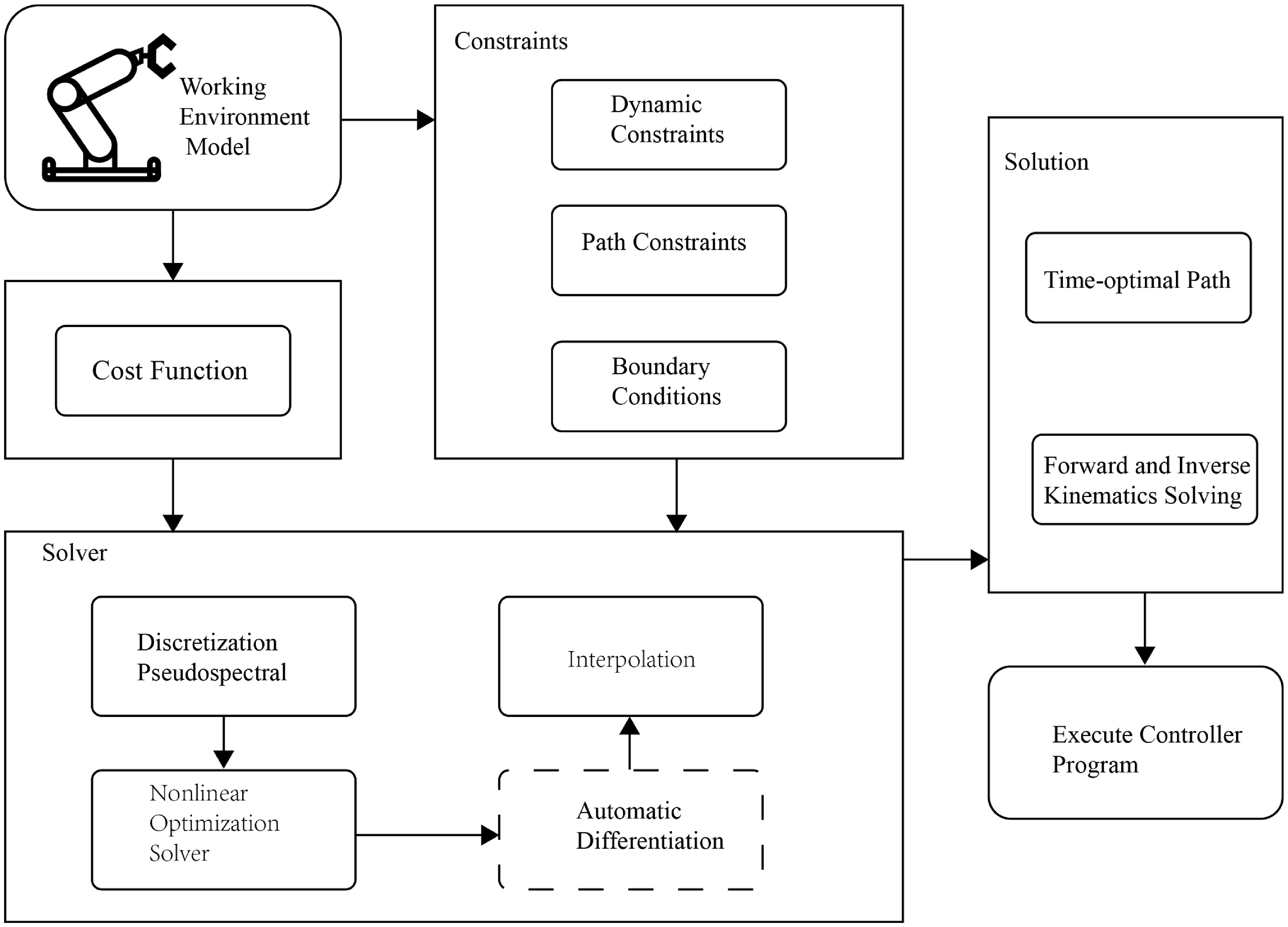
Path optimization is an important part of robotics research, and its optimization results have a crucial impact on the performance of the control system [Reference Wang, Wang, Li, Cai and Wang22, Reference Riboli, Jaccard, Silvestri, Aimi and Malara23]. In most numerical methods, the continuous-time optimal control problem was first transformed into a nonlinear programming problem [Reference Abdelkhalik, Zou, Robinett, Bacelli, Wilson and Coe24]. Then, it was solved with a universal optimization solver. Finally, the approximate solution of the continuous-time optimal control problem was obtained by the polynomial interpolation method. In the numerical approach of path optimization, discretization and optimization played key roles. In recent years, the pseudospectral method has became one of the most important methods to solve the optimal control problem. The Figure 3. describes the robot path optimization process based on the pseudospectral method. The algorithm begins by defining the working environment model, which includes the robot’s operating environment and calculates the cost function to quantify the optimization objectives, typically focusing on minimizing time, energy, or improving motion efficiency. The algorithm takes into account dynamic constraints, path constraints, and boundary conditions, ensuring that the robot moves within specified speed, acceleration, and trajectory limits, from the start to the target. In the solving phase, the pseudospectral discretization method transforms the continuous optimal control problem into a nonlinear programming problem, which is then solved using a nonlinear optimization solver. Interpolation methods ensure path smoothness, while automatic differentiation techniques accelerate the computation. Finally, forward and inverse kinematics solving is used to determine the position and orientation of the robot’s end-effector, and the optimized path is executed by the controller program, ensuring the robot performs tasks efficiently and accurately in complex environments.
Algorithm flowchart for adaptive weight pseudospectral method.

3.1. Discretization of the robot time-optimal problem
In the method of selecting discrete nodes, both the state and control paths are obtained through polynomial approximation parameterization. This approach ensures the smoothness of the path. However, when using higher-order Lagrange polynomials to interpolate a group of nodes, oscillation phenomena may occur. To alleviate this problem, special interpolation nodes can be employed. This involves globally configuring discrete nodes, a technique known as the pseudospectral method.
The pseudospectral method is applied to transform the continuous-time optimal control problem into a nonlinear programming problem. Specifically, it transforms the problem into planning tasks with decision variables
 $x(t),u(t)$
, and
 $t_f$
. The main advantage of this method is its fast convergence and high accuracy when solving path optimization problems [Reference Keil, Kumar and Rao25].
3.1.1. Selection of interpolation nodes
When using the pseudospectral method, the functions requiring approximations are mapped within the interval
 $k\in [-1,1]$
, and the motion time range, the state and the control path time of the robot completing a path are all defined within the interval
 $T\in [0,t_f]$
. Therefore, the process of mapping can enable the following:
 \begin{equation} k=2\frac {T}{t_f} -1 \end{equation}
In the pseudospectral method, the knots
 $(\kappa _i,i=0,1,\ldots ,n)$
can serve as the roots of orthogonal polynomials. Using interpolation knots provided by Chebyshev polynomials not only improves the accuracy of Lagrange interpolation polynomials but is also computationally efficient. This paper employs Chebyshev orthogonal polynomials for calculations. The following expressions define the Chebyshev polynomials
 $y_n(x)$
and knots:
 \begin{align}&\quad\,\, y_n(x)=\cos (n(\cos ^{-1}x)) \end{align}
 \begin{align}& \kappa _i=\cos \left(\frac {i\pi }{n} \right),\quad i=0,\ldots ,n \end{align}
For
 $t\in [t_0,t_f]$
, the knot expression is as follows:
 \begin{equation} T_i=\frac {t_f}{2}\left[\cos \left(\frac {i\pi }{n} \right)+1\right],\quad i=0,\ldots ,n \end{equation}
3.1.2. Lagrange polynomial interpolation
The traditional Lagrange interpolation polynomial can be expressed as:
 \begin{equation} p_j(t)=\sum _{j=0}^{n} L_j(t)f(t_f) \end{equation}
 $L_j(t)$
is the
 $j_{th}$
Lagrange interpolation polynomial, as follows:
 \begin{equation} L_j(t)=\frac { {\textstyle \prod _{m=0,m\neq j}^{n}(t-t_m)} }{{\textstyle \prod _{m=0,m\neq j}^{n}(t_j-t_m)}} \end{equation}
The properties satisfied by Lagrange interpolation polynomial:
 \begin{equation} L_j(t_k)=\begin{cases}1,&j=k \\0,&j\neq k\end{cases} \end{equation}
In order to solve the problems of high computational complexity and numerical instability in traditional Lagrange interpolation polynomial. Trefethen and Liu [Reference Trefethen26, Reference Liu, Huang and Zhang27] improved the traditional Lagrange interpolation polynomial using the idea of center of gravity weight, effectively solving the above problems. The Eq. (17) can be changed by defining the gravity weight to Eq. (19-21):
 \begin{align}&\qquad\,\, \sum _{j=0}^{n} L_j(t)=L(t)\sum _{j=0}^{n}\frac {w_j}{t-t_n}\\[-10pt]\nonumber \end{align}
 \begin{align}&\quad\,\, L(t)=(t-t_0)(t-t_1)\cdots (t-t_n)\\[-10pt]\nonumber \end{align}
 \begin{align}& w_j=\frac {1}{\sum _{m=0,m\neq j}^{n}(t_j-t_m) },\quad j=0,\ldots ,n \end{align}
where
 $w_j$
is the center of gravity weight value. According to interpolation polynomial properties, it is known that
 $\sum _{j=0}^{n}L_j(t)=1$
. Eq. (19) is divided by this formula, get Eq. (22) :
 \begin{equation} L_j(t)=\frac {w_j/t-t_j}{\sum _{m=0}^{n}\frac {w_m}{t-t_m}} ,\quad j=0,\ldots n \end{equation}
The center of gravity weight value doesn’t affect the Lagrange interpolation polynomial result, and when the Chebyshev knots are selected, the gravity weight value can be simplified to:
 \begin{equation} w_j=(-1)^j\upsilon ,\upsilon _j=\begin{cases}1,&j=1,2,\ldots n-1 \\0.5,&j=0,n\end{cases} \end{equation}
The
 $j_{{\rm th}}$
Lagrange polynomial is:
 \begin{equation} L_j(t)=\frac{(-1)^j}{t-t_f}\Big/{\sum _{m=1}^{n-1}\frac {(-1)^m}{t-t_m}+\frac {1}{2}\left(\frac {1}{t-t_0}+\frac {(-1)^n}{t-t_n}\right)} ,\quad j=0,1,2,\ldots n \end{equation}
For the state and the control path, the equation is:
 \begin{align} x(t)\approx \sum _{j=0}^{n} L_j(t)x(t) \nonumber\\ u(t)\approx \sum _{j=0}^{n} L_j(t)u(t) \end{align}
3.1.3. Calculation of standard terms
The standard term of the integral numerical calculation can be obtained using the quadrature method, and the integral term of
 $(\dddot \theta (t))^2B$
in the objective function is approximated by using the quadrature rule in the pseudospectral method:
 \begin{equation} J=t_f+u\int _{0}^{t_f} (\dddot \theta (t))^2B\,{\rm d}t=t_f+u\sum _{j=0}^{n} \omega _j((\dddot \theta (t))^2B) \end{equation}
where
 $\{\omega _j,j=0,\ldots ,n\}$
is a set of creature weights, which is defined as [Reference Waldvogel28]:
 \begin{equation} \omega _j=\int _{0}^{t_f}L_j(t)\,{\rm d}t,\quad j=0,\ldots ,n \end{equation}
Integration Eqs. (24) and (27), the
 $j_{{\rm th}}$
Lagrange interpolation polynomial is written as a function of, and when choosing Chebyshev points, the quadrature rule is Clenshaw-Curtis integration, and Eq. (28) can be integrated as:
 \begin{equation} \begin{aligned}\omega _j&=\int _{0}^{t_f}L_j(t)\,{\rm d}t=\frac {t_f}{2}\int _{-1}^{1}l_j(\kappa )\,{\rm d}\kappa\\&=\frac {t_f}{2}\int _{-1}^{1}\frac {(-1)^j}{\kappa -\kappa _j}+\frac {1}{2}\left(\frac {1}{\kappa -\kappa _0}+\frac {(-1)^n}{\kappa -\kappa _n} \right )\,{\rm d}\kappa\\&=\frac {t_fd_j}{2n}\left ( 1-\sum _{m=1}^{n/2} \frac {g_m}{4m^2-1}\cos (2m\kappa _j) \right ) ,\quad j=0,1,\ldots ,n \end{aligned} \end{equation}
where
 $g_m=\begin{cases}1,&m=\dfrac {n}{2}\\ 2,&m\lt \frac {n}{2}\end{cases}$
,
 $d_j=\begin{cases}1,&j=0,n\\ 2,&j=1,2,\ldots ,n\end{cases}$
3.1.4. Calculation of the derivative matrix at nodes.
The state and control path formula of the corresponding stacking knots during the movement of the robot are expressed as:
 \begin{equation} X=\begin{bmatrix}x(T_0)^T\\ .\\ .\\ .\\x(T_n)^T\end{bmatrix},\quad U=\begin{bmatrix}u(T_0)^T\\ .\\ .\\ .\\u(T_n)^T\end{bmatrix} \end{equation}
The state and control derivatives at knots are approximated calculation by polynomials, which can be expressed as:
 \begin{equation} \frac {d}{d_t} X=\frac {2}{t_f} DX,\frac {d}{d_t}U=\frac {2}{t_f}DU \end{equation}
 $D$
is the differential matrix for calculating the derivative of
 $X$
and
 $U$
with respect to
 $\kappa \in [-1,1]$
[Reference Liu, Huang and Zhang27]. Each element of the differential matrix is calculated using the following formula:
 \begin{equation} D_{ij}=\left \{\begin{matrix}\frac {W_j/w_i}{\kappa _i -\kappa _j } ,&i\neq j \\-\sum _{i\neq j}^{} D_{ij},&i=j\end{matrix}\right . \end{equation}
Let
 $X=\begin{bmatrix}x(T_0)^T\\ .\\ .\\ .\\x(T_n)^t\end{bmatrix}$
,
 $\Phi =\begin{bmatrix}F(x(T_0)^T,u(T_0)^T)\\ .\\ .\\ .\\F(x(T_n)^T,u(T_n)^T)\end{bmatrix}$
the dynamic constraints of discrete nodes are represented by differential matrix:
 \begin{equation} DX-\frac {t_f}{2} \Phi =0 \end{equation}
3.2. Convergence analysis of adaptive weight iteration
In the pseudospectral trajectory optimization framework proposed in this paper, the acceleration weighting vector
 $\textbf{u} \in \mathbb{R}^m$
is updated iteratively in an adaptive manner. The update rule for the weights is based on the maximum joint accelerations of the current trajectory, formulated as:
 \begin{equation} u_i^{k+1} = f_i\left ( \max _{t \in [0,T]} \left | \ddot {q}_i^k(t) \right | \right ), \quad i=1, \ldots , m, \end{equation}
where
 $\ddot {q}_i^k(t)$
denotes the acceleration trajectory of the
 $i$
-th joint at the
 $k$
-th iteration, and the function
 $f_i: \mathbb{R} \to \mathbb{R}$
defines the scalar weight update for each component.
To analyze the convergence of this iterative process, we define the overall weight update mapping as:
 \begin{equation} \textbf{u}^{k+1} = F(\textbf{u}^k) := f\big ( a(\textbf{u}^k) \big ), \end{equation}
where
 \begin{equation} a(\textbf{u}) := \max _{t \in [0,T]} |\ddot {\textbf{q}}(t; \textbf{u})| \in \mathbb{R}^m, \end{equation}
is the vector of maximum joint accelerations dependent on the weight parameter
 $\textbf{u}$
, and the mapping
 $f = (f_1, \ldots , f_m)$
acts component-wise on
 $a(\textbf{u})$
.
We assume the following Lipschitz continuity conditions hold:
-
1. The mapping from weights to maximum accelerations is Lipschitz continuous, that is, there exists a constant
 $L_a \gt 0$
such that(36)where
\begin{equation} \| a(\textbf{u}) - a(\textbf{v}) \| \leq L_a \| \textbf{u} - \textbf{v} \|, \quad \forall \textbf{u}, \textbf{v} \in \mathcal{U}, \end{equation}
$\mathcal{U} \subset \mathbb{R}^m$
is a bounded neighborhood of the weights.
-
2. The weight update function
$f$
is Lipschitz continuous with constant
$L_f \gt 0$
, that is,(37)
\begin{equation} \| f(\textbf{x}) - f(\textbf{y}) \| \leq L_f \| \textbf{x} - \textbf{y} \|, \quad \forall \textbf{x}, \textbf{y} \in f(\mathcal{U}). \end{equation}


Consequently, the composite mapping
 $F$
satisfies
 \begin{equation} \| F(\textbf{u}) - F(\textbf{v}) \| = \| f(a(\textbf{u})) - f(a(\textbf{v})) \| \leq L_f \| a(\textbf{u}) - a(\textbf{v}) \| \leq L_f L_a \| \textbf{u} - \textbf{v} \|. \end{equation}
If the contraction condition
 \begin{equation} L := L_f L_a \lt 1 \end{equation}
is satisfied, then by the Banach fixed-point theorem, the mapping
 $F$
has a unique fixed point
 $\textbf{u}^*$
in
 $\mathcal{U}$
such that
 \begin{equation} \textbf{u}^* = F(\textbf{u}^*). \end{equation}
Furthermore, for any initial weight
 $\textbf{u}^0 \in \mathcal{U}$
, the iterative sequence
 $\{\textbf{u}^k\}$
converges to
 $\textbf{u}^*$
with the geometric rate:
 \begin{equation} \| \textbf{u}^k - \textbf{u}^* \| \leq L^k \| \textbf{u}^0 - \textbf{u}^* \|. \end{equation}
In cases where the contraction condition is not initially met, a damping strategy can be employed to guarantee convergence:
 \begin{equation} \textbf{u}^{k+1} = (1 - \alpha ) \textbf{u}^k + \alpha F(\textbf{u}^k), \quad \alpha \in (0,1). \end{equation}
In summary, the convergence of the adaptive weight iteration proposed in this paper is guaranteed under the above Lipschitz continuity assumptions, providing a solid theoretical foundation for the stability and effectiveness of the trajectory optimization algorithm.
3.3. Automatic differentiation
Many optimization solvers are based on the gradient descent algorithm, which iteratively updates the parameters in the direction of steepest descent of the objective function [Reference Nazmara and Ahmadi29]. The derivatives of the objective and constraint functions are typically computed using numerical differentiation methods, which is computationally expensive and prone to rounding errors. Symbolic differentiation is inefficient for functions of high-dimensional matrices, while both numerical and symbolic differentiation have issues in computing high-order derivatives.
In order to improve the computational efficiency of numerical methods and solve problems in numerical differentiation and symbolic differentiation, the automatic differentiation method is introduced, which is a technique for quickly calculating accurate derivatives. The automatic differentiation method is based on the implementation of even number algorithms, while for even numbers, it is an extension of real numbers, similar to introducing an imaginary number to increase the real number
 $\vartheta$
for complex numbers, such as
 $\vartheta ^2=-1$
. However, this method introduces an infinitesimal element
 $\varepsilon$
for even numbers, that is
 $\varepsilon ^2=0$
. Using Taylor expansion, the function value is calculated as:
 \begin{equation} f(x+\varepsilon )=f(x)+\sum _{i=1}^{\infty }\frac {f^i(x)}{i!} \varepsilon ^2=f(x)+f^1(x)\varepsilon \end{equation}
where
 $f^i(x)$
is the
 $i_{{\rm th}}$
derivative of function
 $f(x)$
. In Eq. ( 43),
 $f(x)$
and
 $f^1(x)$
are the two components of the returned double number. Similarly, more dual components are introduced to achieve functionality. The computational cost of automatic differentiation is much lower than that of numerical differentiation or symbolic differentiation. CasADi is an open-source numerical solver library that provides a set of algorithms for integration and nonlinear optimization. It is used for various dynamic and control system models [Reference Elhesasy, Dief, Atallah, Okasha, Kamra, Yoshida and Rushdi30] and quickly integrated into various popular mathematical modeling and programming environments. Therefore, in this paper, the CasADi solver is chosen to accurately calculate the derivatives of the functions used.
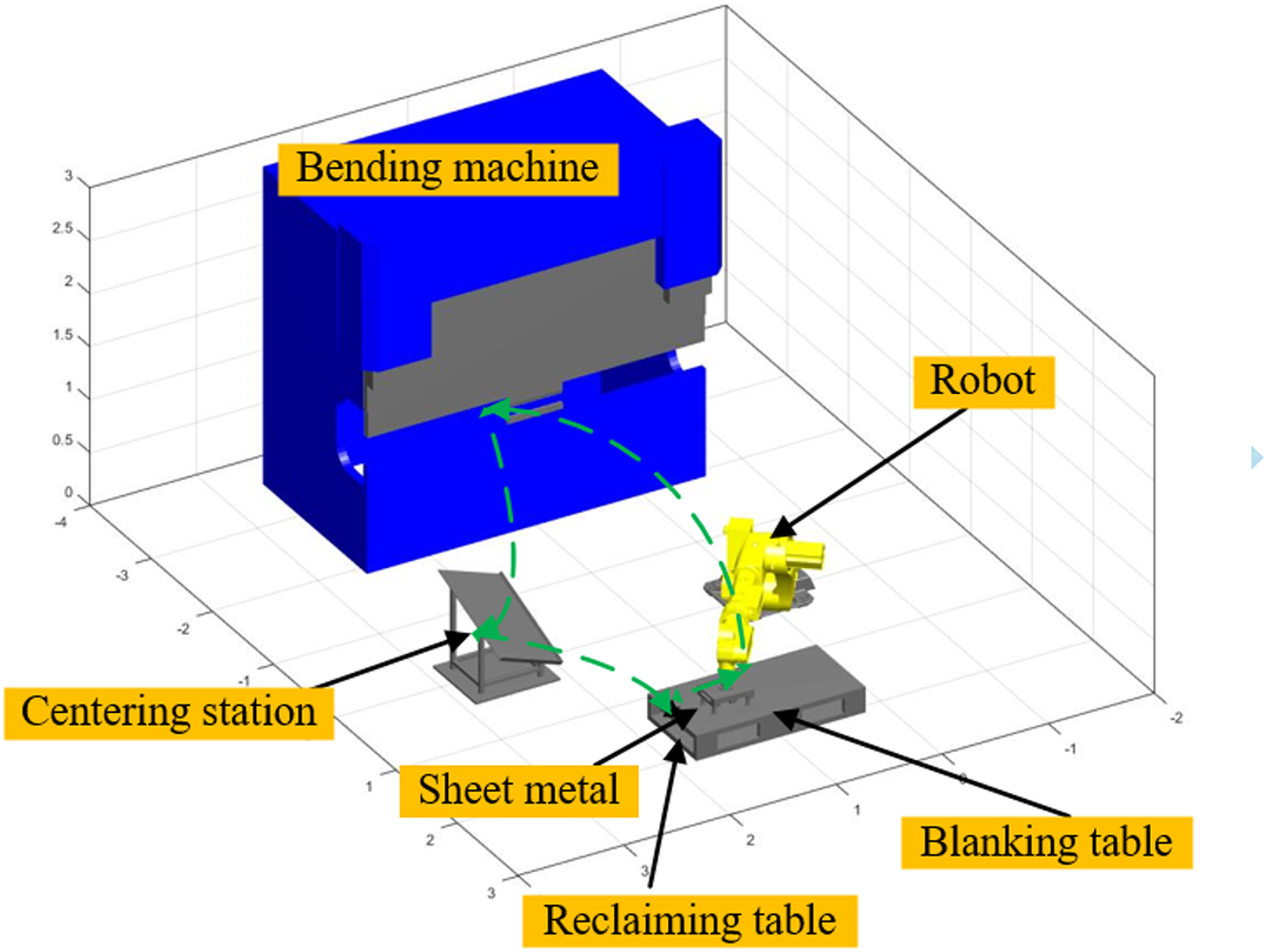
Sheet metal bending process on-site environment 3D model.

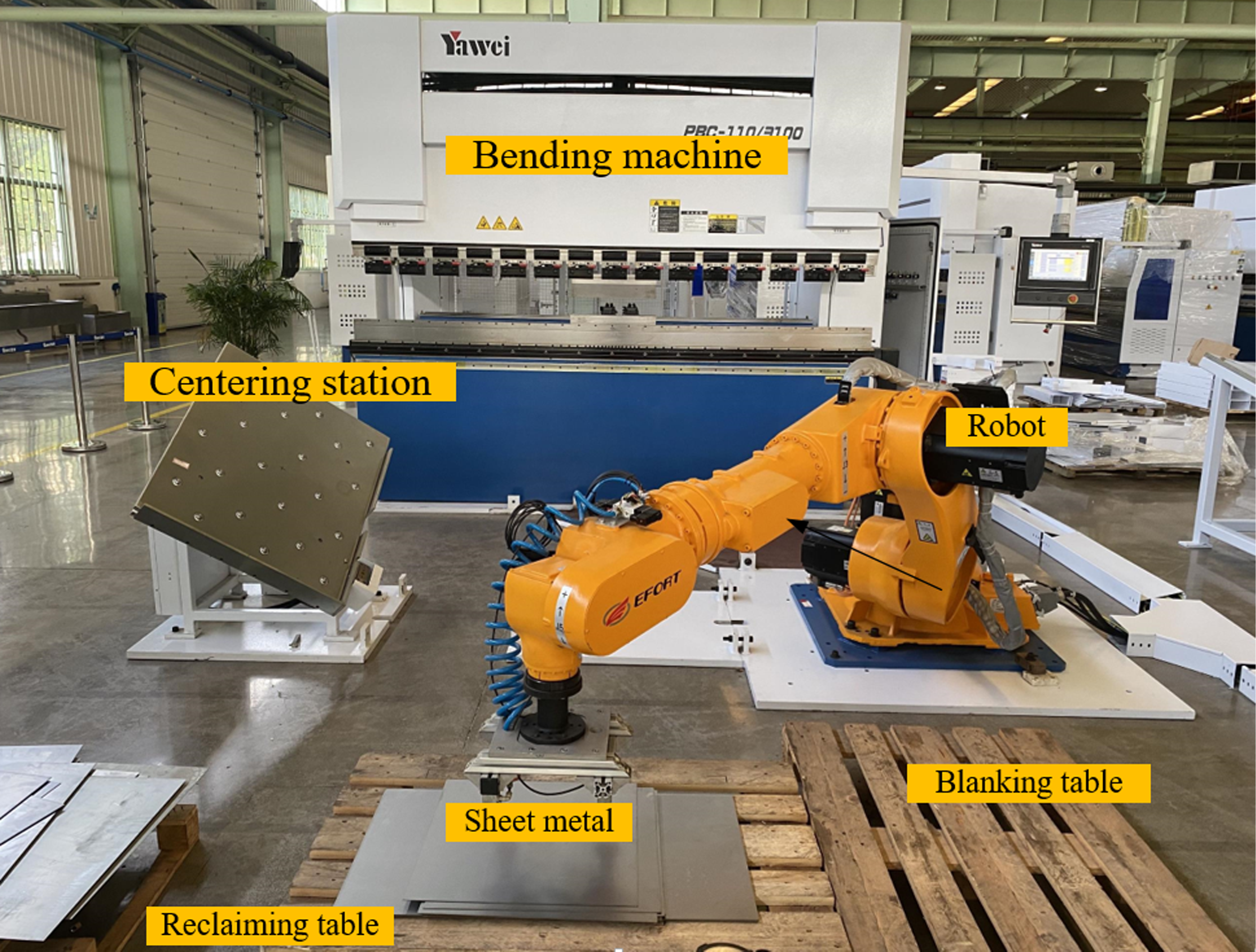
Actual processing environment for the sheet metal bending process.

4. Simulations and experiments
This section presents two sets of simulation and experimental comparisons between the proposed pseudospectral-based path optimization algorithm and a traditional algorithm [Reference Zhao, Lin and Tomizuka11], with the objective of minimizing the time. The simulation and experimental environments have consistent constraints. To avoid the randomness in robot operation, all the displayed experimental results in this section are the average of 50 trials. The simulation and experimental environments are based on a robotic sheet metal bending manufacturing environment. The process involves the robot grasping the sheet metal and moving it to the centering station for physical alignment. Then, the robot grabs the sheet metal and moves it to the bending machine’s lower die surface for bending. The formed sheet metal is then moved to the unloading station for material removal. Finally, the robot returns to the original position. The 3D models of the robot body, bending machine, centering station, loading station, unloading station, and other components are shown in Figure 4, while the actual manufacturing environment is shown in Figure 5.
4.1. Comparison with fixed-weight pseudospectral algorithm
Given the initial angle of each joint of the robot
 $\theta _0$
and end angle
 $\theta _f$
. Under the conditions of satisfying the state Eq. (10), path constraints, boundary constraints (Table I, Table II), and obstacle constraints solve the control variable
 $u(t)$
to minimize the calculation result of the objective Eq. (3). First, the optimal control problem is discretized and approximated to a nonlinear constrained optimization problem, and then the CasADi solver based on MATLAB is used to solve the nonlinear constrained optimization problem.
This research conducts two sets of comparative simulations between the new path optimization algorithm and traditional algorithms, with the objective of achieving time optimization. The simulation environment and constraint conditions are kept consistent. The hardware environment used for testing is a personal computer equipped with an Intel(R) Core(TM) i5-9400F CPU (2.90 GHz) and 16 GB of memory. The software environment is MATLAB R2018b running on Windows 10. Considering that the weighting coefficients of traditional algorithms are constant, the comparison mainly includes calculation time, iteration times, and target values. Set the path planning time
 $t_f$
=0.5s, and the number of Chebyshev interpolation knots
 $n$
=12.
Case 1 Start point:
 $\theta _0=[51.63^\circ ,-58.30^\circ ,-24.67^\circ ,0^\circ ,82.96^\circ ,-38.37^\circ ]^T$
Termination point:
 $\theta _f=[51.63^\circ ,-56.70^\circ ,-22.63^\circ ,0^\circ ,79.33^\circ ,-38.37^\circ ]^T$
The first set of simulation comparison data.

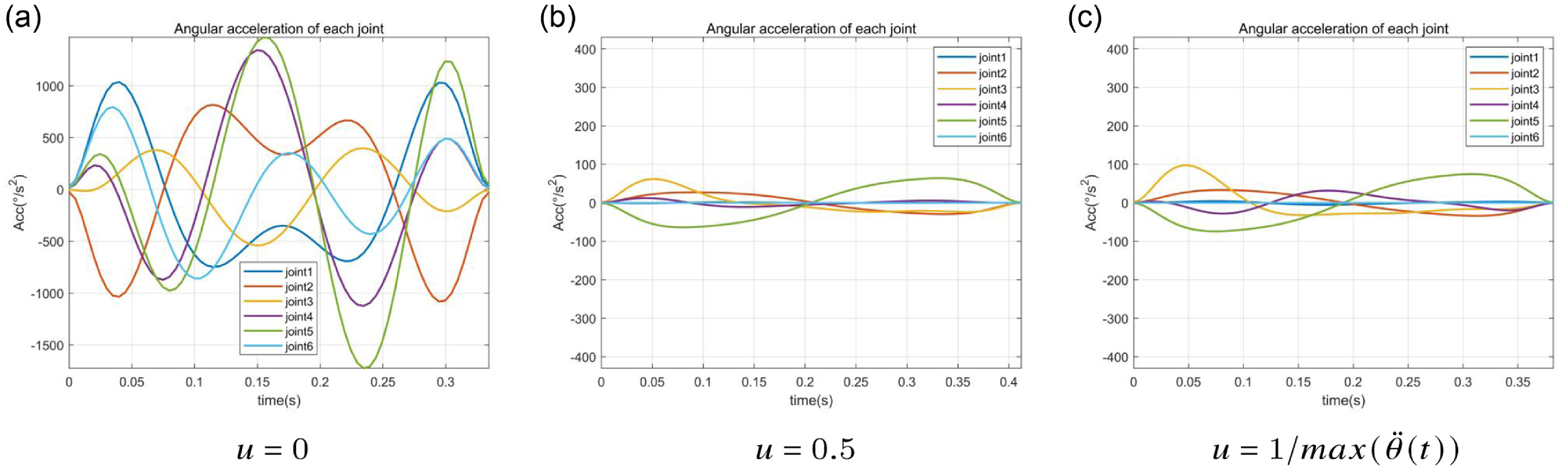
The comparative data of Case 1 are shown in Table III. Based on the data obtained from the simulation, it is found that when the weight value
 $u \gt 0.5$
, the target values gradually become larger, which does not meet the selection criteria. Therefore,
 $u=0$
and
 $u=0.5$
were chosen for comparison with the acceleration curves under the adaptive weight values in this paper; the results are shown in Figure 6.
The second set of simulation comparison data.

Case 1: Joint angle acceleration with different weight values
 $u$
.

Case 2 Start point:
 $\theta _0=[51.63^\circ ,-58.30^\circ ,-24.67^\circ ,0^\circ ,82.96^\circ ,-38.37^\circ ]^T$
Termination point:
 $\theta _f=[11.42^\circ ,-74.76^\circ ,-12.46^\circ ,-38.41^\circ ,52.79^\circ ,13.75^\circ ]^T$
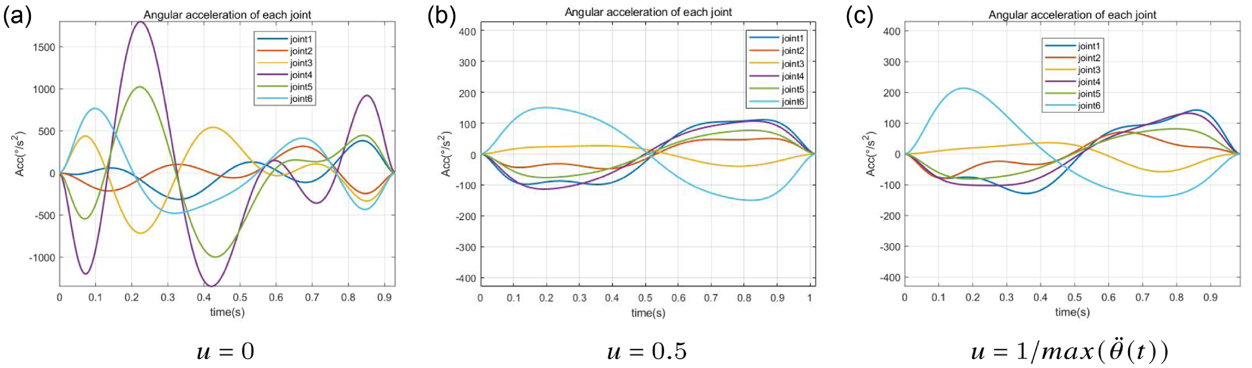
The comparative data of Case 2 are shown in Table IV. In the same environment, a second set of data simulations was conducted, comparing the acceleration results for three different weight values:
 $u=0$
,
 $u=0.5$
, and
 $u=1/max(\ddot \theta (t))^2$
. The results are shown in Figure 7.
Performance comparison between AWPM, WOA, and PSO.

Case 2:Joint angle acceleration with different weight values
 $u$
.

4.2. Comparison with intelligent optimization algorithms
To further evaluate the performance and novelty of the proposed algorithm, we conducted comparative simulations between our method and two intelligent optimization algorithms: the Whale Optimization Algorithm (WOA), a novel nature-inspired heuristic, and the PSO algorithm, a classical population-based optimization method.
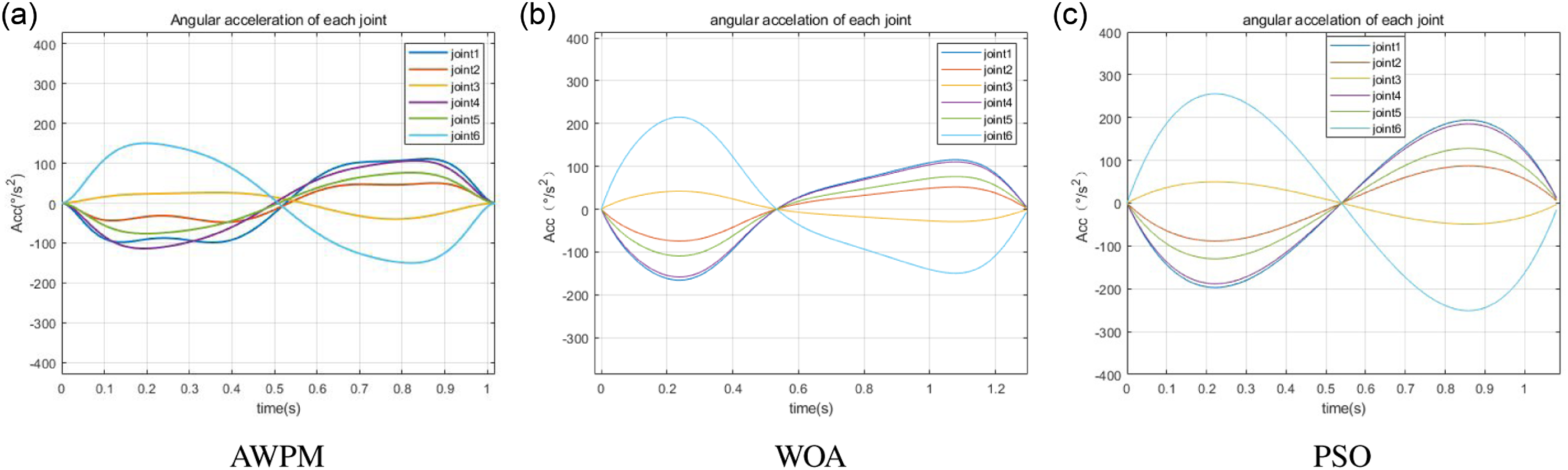
To ensure the reliability and comparability of the results, all simulations were conducted under identical conditions: using the same ER80-2600 robot model, the same constraint settings, and the same cost function formulation as adopted throughout this study. The comparison specifically focused on Case 2 from Section 4.1, using its initial and final joint configurations as the test scenario. The simulation results for the same iterations are summarized in Table V.
In the comparison, the proposed algorithm – Adaptive Weighted Pseudospectral Method (AWPM) –employs an adaptive mechanism to adjust the weight of the cost function during optimization. In contrast, both WOA and PSO use a fixed weight
 $u = 1$
, with no adaptive adjustment mechanism. As shown in Table V, although heuristic methods such as WOA and PSO can explore a wide solution space, they do not exploit gradient information and rely on stochastic sampling, which often results in slower convergence.
By discretizing the optimal control problem into a nonlinear programming problem, AWPM leverages gradient and second-order derivative information, enabling significantly faster and more stable convergence to the optimal solution. Compared to WOA and PSO, AWPM improved computation time by 10.56% and 44.90%, respectively, and achieved a 48.32% and 19.01% improvement in the precision of the objective value convergence.
As shown in Figure 8, the joint angular acceleration curves of the three algorithms under Case 2 indicate that AWPM not only accelerates convergence by effectively leveraging the problem structure, but also reduces acceleration fluctuations, thereby improving the solution quality. This demonstrates that AWPM is a more effective method for time-optimal path planning under complex constraints.
Joint angular acceleration curves for AWPM, WOA, and PSO.

4.3. Simulation
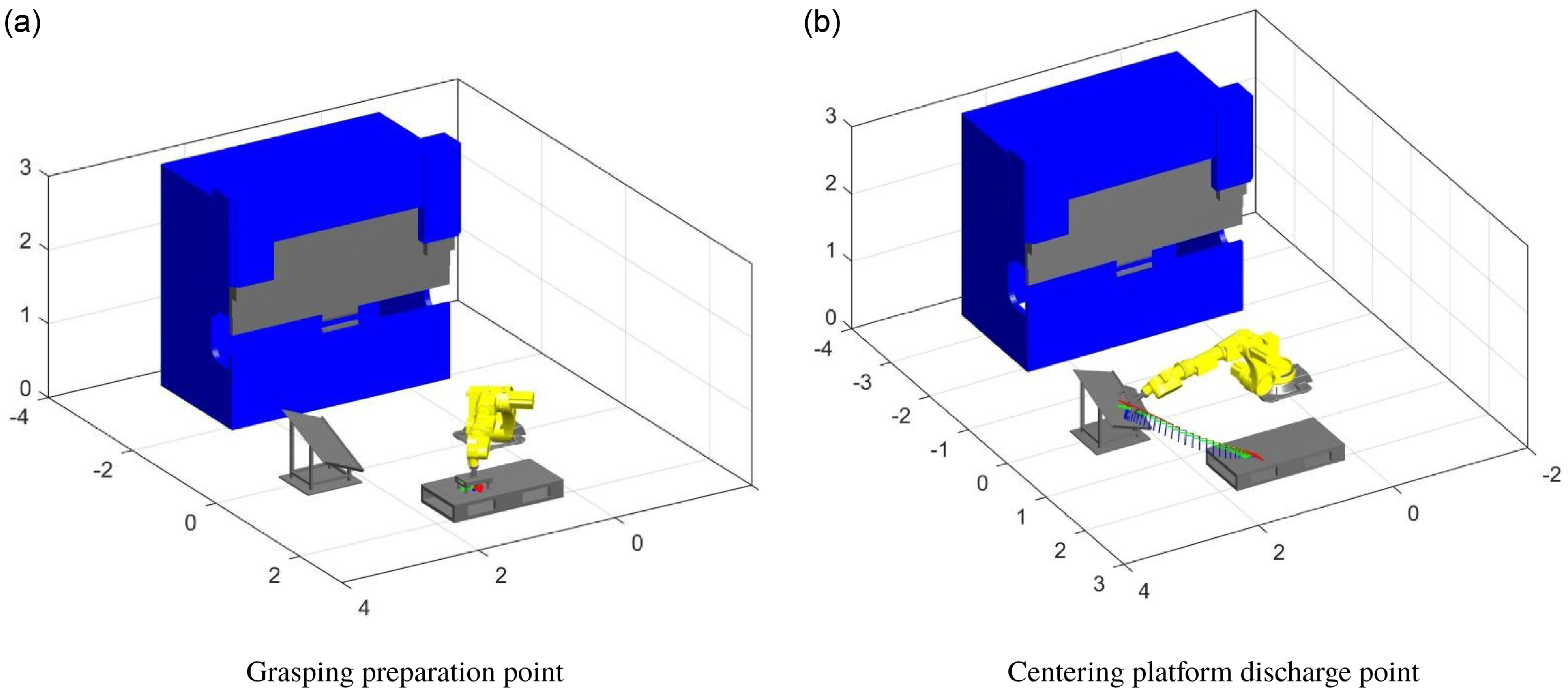
This section focuses on simulating the process of the robot grasping the sheet metal and moving it to the centering platform to achieve physical alignment. The motion process of the robot is shown in Figure 9.
Actual processing environment for the sheet metal bending process.

Set the path planning time to
 $t_f$
=0.5s, the number of Chebyshev interpolation nodes to
 $n$
=12, and the starting each joint angle
 $\theta _0$
and ending each joint angle
 $\theta _f$
of the robot are respectively:
Start point:
 $\theta _0=[51.63^\circ ,-56.70^\circ ,-22.63^\circ ,0^\circ ,79.33^\circ ,-38.37^\circ ]^T$
Termination point:
 $\theta _f=[9.49^\circ ,-65.81^\circ ,-18.83^\circ ,-38.63^\circ ,49.58^\circ ,13.88^\circ ]^T$
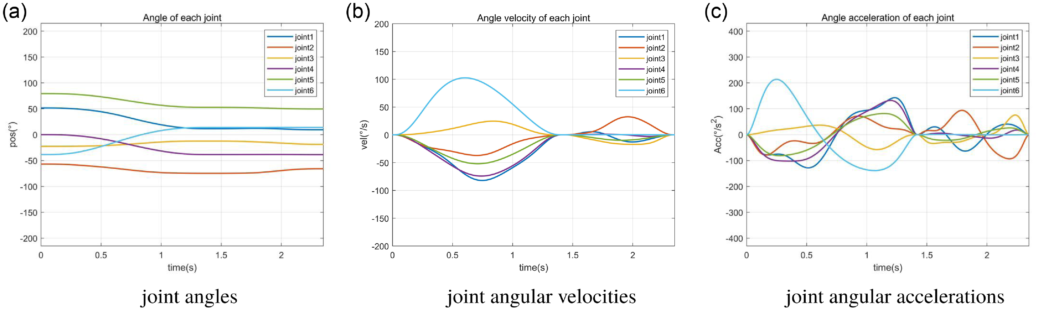
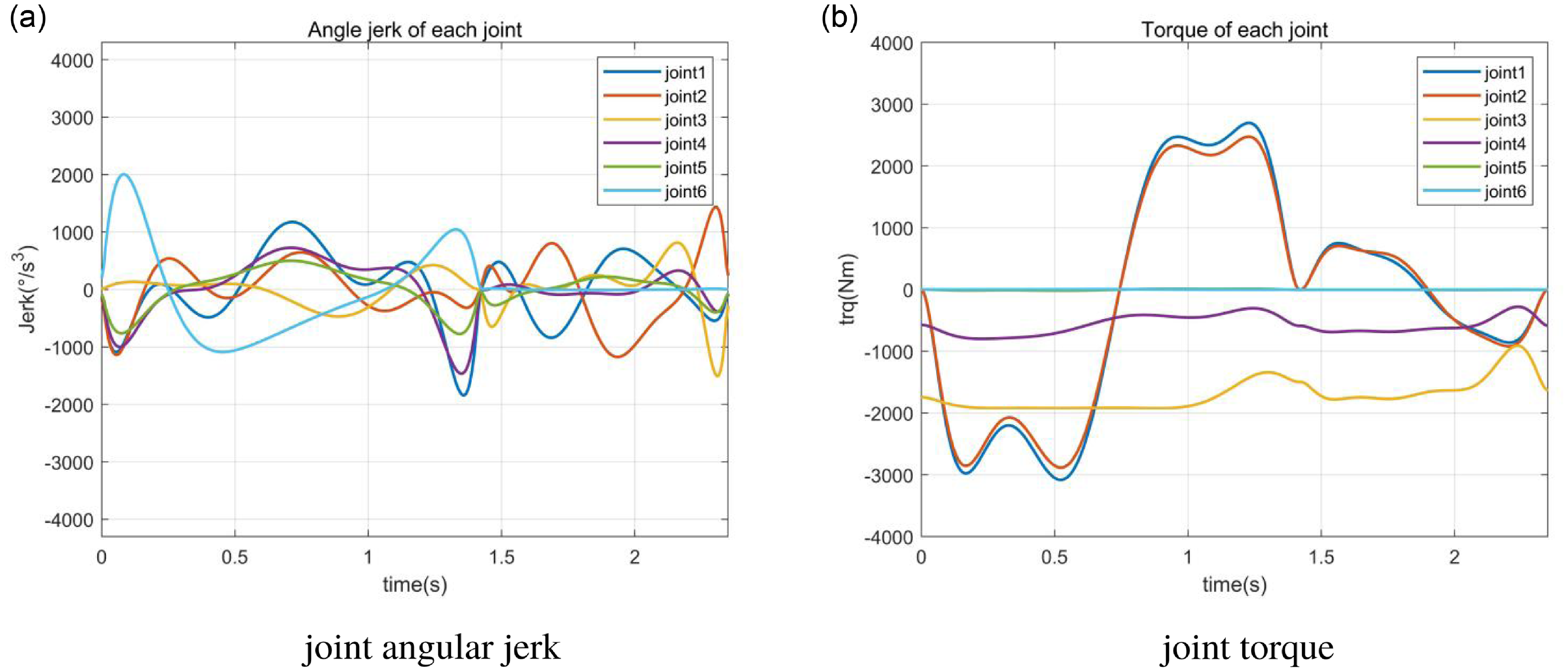
The simulation results are shown in Figures 10 and 11. Among them, Figure 10(a)–(c) represents the motion data curves of the robot joint angles, angular velocities, and angular accelerations during this process of the robot from the grasping point to the centering platform. Figure 11a shows the motion data curve of angular jerk during this process. Figure 11b shows the motion data curve of the torque of each joint of the robot during this process.
In the above simulation example, under the determined constraints, after a computer running time of 0.478s and 67 iterations, the target value was reached, and the performance index function value.
Motion curve of the robot.

Motion curve of the robot.

4.4. Experimental result
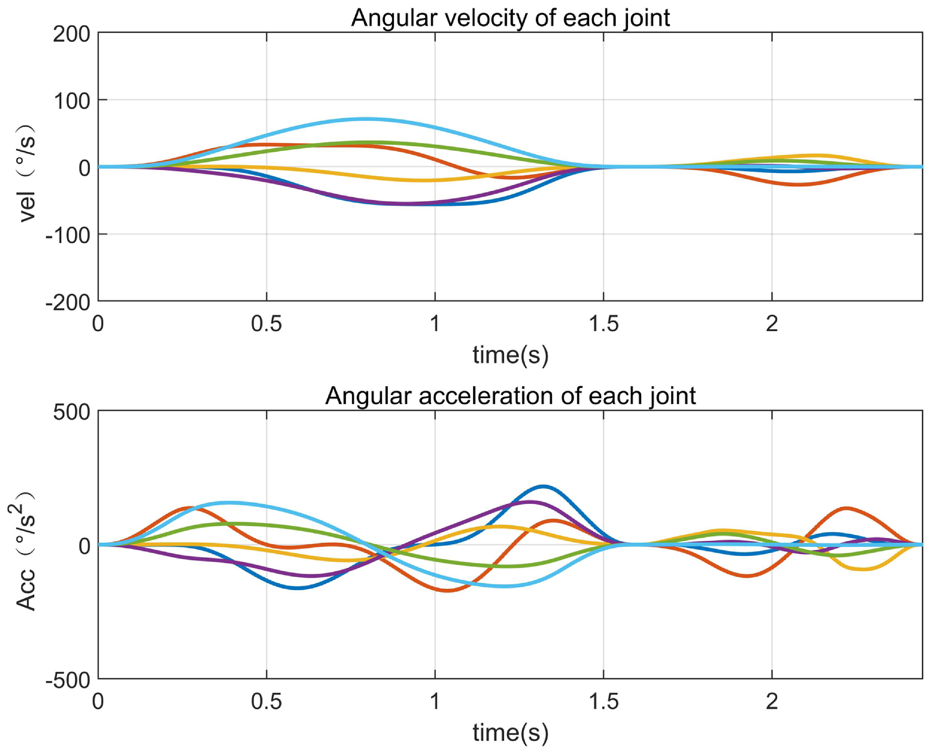
To verify the accuracy of the simulation results, this paper used the ER80-2600 robot to verify the algorithm. The on-site environmental conditions were consistent with the Section 4.3 simulation environment. The controller program instructions were used to control the robot to move in the joint space according to the joint angle data obtained from the simulation, and actual motion data of each joint were collected.
The state of the robot at different times during the motion process.

Angular velocity and angular acceleration during the robot motion process.

Figure 12 represents the robot’s states at different time points (t) during the process of the selected robot grasping the sheet metal and moving toward the center of the platform. The motion data for each joint during this process are obtained from the robot control system, ROBOX, and the results are shown in Figure 13.
The actual running time of the robot can be obtained from the robot’s teach pendant control panel, which is 2.448s.
5. Discussion
By analyzing Cases 1 and 2, it is evident that using traditional algorithm for path planning with weight coefficient
 $u=0$
, the robot has the shortest running time but requires more iterations. It results in slower computational efficiency. Additionally, the peak angular acceleration during robot operation exceeds the constraint range, as shown in Figures 6(a) and 8(a). As the weight coefficient
 $u$
increases, the number of iterations decreases, but the robot’s running time increases, as shown in Tables III and IV. It also means that the value of
 $u$
cannot be determined for different working conditions. However, when using the path optimization algorithm based on the pseudospectral method proposed in this paper, the appropriate value of
 $u$
is automatically adjusted according to the working conditions. This approach reduces the number of iterations and improves computational efficiency, enabling shorter robot run times and faster identification of high-quality paths.
The proposed algorithm was simulated and tested on the robot using MATLAB, as shown in Figures 10 and 11. During the robot’s motion, the velocities, accelerations, jerk, and torque of each joint are within the constraint range. The entire process is fast, smooth, and collision-free. Moreover, the actual running time during robot motion is consistent with the average running time in the ROBOX controller, which is approximately 2.448s. However, it slightly deviates from the simulated robot running time in MATLAB, which is 2.35s, as shown in Figures 13 and 10(a). This discrepancy is attributed to factors such as friction and external influences experienced by the robot in the actual operating environment, resulting in some errors in the running time. The simulation and experimental results validate the generality and feasibility of the path optimization algorithm based on the proposed pseudospectral method.
6. Conclusion
This research proposes an adaptive weighted pseudospectral algorithm for robot path planning to enhance efficiency. The objective function incorporates an adaptive weight to optimize path quality, while the collision detection model uses five-separating-axes intersection detection to improve computational efficiency. Simulation and experimental results demonstrate that the algorithm generates time-optimal trajectories, ensuring stability and boosting work efficiency. Its potential applications in industrial robots promise optimized paths and increased productivity.
Supplementary material
The supplementary material for this article can be found at https://doi.org/10.1017/S0263574725102063.
Author contributions
Conceptualization and methodology, W.Z.; software, Z.G.; validation, W.Z., Z.G., and X.S.; writing – original draft preparation, W.Z. and Z.G.; writing – review and editing, W.Z. and Z.G.; visualization, Z.G.; supervision, L.F.; project administration, L.F.; All authors have read and agreed to the published version of the manuscript.
Financial support
This research was supported by the Jiangsu(Industry Foresight and Key Core Technology) Key R&D Project [Grant No. BE2022137].
Competing interests
The authors declare no conflicts of interest exist.
Ethical approval
Not applicable.