2.1 Governing equations, base flow, direct and adjoint global modes

The governing equations are considered in a general way as

(2.1) $$\begin{eqnarray}\frac{\text{d}\boldsymbol{q}}{\text{d}t}=\boldsymbol{R}(\boldsymbol{q}),\end{eqnarray}$$

where $\boldsymbol{R}$ is the spatially discretized residual and $\boldsymbol{q}$ the state variable containing, for example in the case of compressible equations the velocity components, the density and temperature fields. In the following, it is considered to have $p$ variables at all points of the mesh. For example, in the case of two-dimensional flows, $p=3$ in the case of incompressible flow fields, $p=4$ if the flow is compressible and $p=5$ if the flow is compressible and a Spalart–Allmaras model used to define an eddy-viscosity.

The steady solution $\boldsymbol{q}_{0}$ of the equations, also called base flow, is a solution of

(2.2) $$\begin{eqnarray}\boldsymbol{R}(\boldsymbol{q}_{0})=0.\end{eqnarray}$$

The dynamics of small amplitude perturbations $\boldsymbol{q}^{\prime }(t)=\hat{\boldsymbol{q}}\exp (\unicode[STIX]{x1D706}t)$ is analysed in the vicinity of $\boldsymbol{q}_{0}$ by considering the eigenproblem associated with the Jacobian matrix

(2.3a,b ) $$\begin{eqnarray}\unicode[STIX]{x1D645}\hat{\boldsymbol{q}}=\unicode[STIX]{x1D706}\hat{\boldsymbol{q}},\quad J_{kl}=\left.\frac{\unicode[STIX]{x2202}R_{k}}{\unicode[STIX]{x2202}q_{l}}\right|_{\boldsymbol{q}=\boldsymbol{q}_{0}},\end{eqnarray}$$

where $\unicode[STIX]{x1D645}$ is the Jacobian matrix associated with $\boldsymbol{R}$ around the base flow, $R_{k}$ the $k$ th component of the residual and $q_{l}$ the state variable at a given location. The quantity $\unicode[STIX]{x1D706}$ describes the temporal behaviour of the perturbation; its real part $\unicode[STIX]{x1D70E}$ is the growth rate and its imaginary part $\unicode[STIX]{x1D714}$ the angular frequency.

The adjoint eigenvalue problem associated with (2.3) is introduced in the following. Let us consider an inner product based on a real symmetric positive definite matrix $\unicode[STIX]{x1D651}$ such that $\langle \boldsymbol{a},\boldsymbol{b}\rangle _{\unicode[STIX]{x1D651}}=\boldsymbol{a}^{\ast }\unicode[STIX]{x1D651}\boldsymbol{b}$ , where $\boldsymbol{a}$ and $\boldsymbol{b}$ are arbitrary vectors and the superscript $^{\ast }$ refers to the transconjugate. In the following, the matrix $\unicode[STIX]{x1D651}$ is chosen so that $\langle \boldsymbol{a},\boldsymbol{a}\rangle _{\unicode[STIX]{x1D651}}$ represents the square of the function $L_{2}$ norm. Also in the following, $\unicode[STIX]{x1D651}$ is a diagonal matrix for which the terms $V_{k}$ correspond to the volume of each cell, as is the case in a finite-volume discretization. The adjoint matrix $\tilde{\unicode[STIX]{x1D645}}$ is defined as

(2.4) $$\begin{eqnarray}\langle \boldsymbol{a},\unicode[STIX]{x1D645}\boldsymbol{b}\rangle _{\unicode[STIX]{x1D651}}=\langle \tilde{\unicode[STIX]{x1D645}}\boldsymbol{a},\boldsymbol{b}\rangle _{\unicode[STIX]{x1D651}}.\end{eqnarray}$$

It is straightforward to show that

(2.5) $$\begin{eqnarray}\tilde{\unicode[STIX]{x1D645}}=\unicode[STIX]{x1D651}^{-1}\unicode[STIX]{x1D645}^{\ast }\unicode[STIX]{x1D651}.\end{eqnarray}$$

It follows that the eigenvalues of $\tilde{\unicode[STIX]{x1D645}}$ are the complex conjugates of those of $\unicode[STIX]{x1D645}$ . Given an eigenvalue/eigenvector pair $(\unicode[STIX]{x1D706},\hat{\boldsymbol{q}})$ , the associated adjoint global mode $\tilde{\boldsymbol{q}}$ is solution of the eigenproblem

(2.6) $$\begin{eqnarray}\tilde{\unicode[STIX]{x1D645}}\tilde{\boldsymbol{q}}=\unicode[STIX]{x1D706}^{\ast }\tilde{\boldsymbol{q}}.\end{eqnarray}$$

An important property used in the following is the bi-orthogonality of the two bases composed by the entire sets of eigenvectors of $\unicode[STIX]{x1D645}$ and $\tilde{\unicode[STIX]{x1D645}}$ with respect to the defined inner product

(2.7) $$\begin{eqnarray}\langle \tilde{\boldsymbol{q}}_{n},\hat{\boldsymbol{q}}_{j}\rangle _{\unicode[STIX]{x1D651}}=\tilde{\boldsymbol{q}}_{n}^{\ast }\unicode[STIX]{x1D651}\hat{\boldsymbol{q}}_{j}=\unicode[STIX]{x1D6FF}_{nj},\end{eqnarray}$$

where $\unicode[STIX]{x1D6FF}_{nj}$ is the Kronecker symbol. It means also that the inner product of a direct eigenvector with its adjoint is normalized to be equal to one.

2.2 Structural sensitivity and wavemaker analysis

The classical way to identify flow regions responsible for a global instability is to perform the wavemaker analysis introduced by Giannetti & Luchini (Reference Giannetti and Luchini2007). This analysis is derived from a structural sensitivity analysis. The Jacobian is perturbed by an arbitrary matrix $\unicode[STIX]{x1D6FF}\unicode[STIX]{x1D645}$ and the eigenproblem (2.3) is modified to (Schmid & Brandt Reference Schmid and Brandt2014)

(2.8) $$\begin{eqnarray}\displaystyle (\unicode[STIX]{x1D645}+\unicode[STIX]{x1D6FF}\unicode[STIX]{x1D645})(\hat{\boldsymbol{q}}+\unicode[STIX]{x1D6FF}\hat{\boldsymbol{q}})=(\unicode[STIX]{x1D706}+\unicode[STIX]{x1D6FF}\unicode[STIX]{x1D706})(\hat{\boldsymbol{q}}+\unicode[STIX]{x1D6FF}\hat{\boldsymbol{q}}), & & \displaystyle\end{eqnarray}$$

where $\unicode[STIX]{x1D6FF}\unicode[STIX]{x1D706}$ and $\unicode[STIX]{x1D6FF}\hat{\boldsymbol{q}}$ denote the eigenvalue and eigenvector variations, respectively. Assuming these variations are small, the eigenvalue variation is straightforwardly obtained through

(2.9) $$\begin{eqnarray}\displaystyle \unicode[STIX]{x1D6FF}\unicode[STIX]{x1D706}=\tilde{\boldsymbol{q}}^{\ast }\unicode[STIX]{x1D651}\unicode[STIX]{x1D6FF}\unicode[STIX]{x1D645}\hat{\boldsymbol{q}}. & & \displaystyle\end{eqnarray}$$

To identify spatial regions of the flow where local feedback is at play in the instability, Giannetti & Luchini (Reference Giannetti and Luchini2007) considered an arbitrary matrix in the form

(2.10) $$\begin{eqnarray}\displaystyle \unicode[STIX]{x1D6FF}\unicode[STIX]{x1D645}=\unicode[STIX]{x1D644}_{k}, & & \displaystyle\end{eqnarray}$$

where $\unicode[STIX]{x1D644}_{k}$ is a diagonal block matrix with all diagonal blocks equal to zero except for the $k$ th cell where it is equal to $\unicode[STIX]{x1D644}_{p,p}$ , the $p\times p$ identity matrix. This choice induces the eigenvalue variation

(2.11) $$\begin{eqnarray}\displaystyle \unicode[STIX]{x1D6FF}\unicode[STIX]{x1D706}_{k}=\tilde{\boldsymbol{q}}_{k}^{\ast }V_{k}\hat{\boldsymbol{q}}_{k}, & & \displaystyle\end{eqnarray}$$

where $V_{k}$ is the volume of cell $k$ , $\hat{\boldsymbol{q}}_{k}$ and $\tilde{\boldsymbol{q}}_{k}$ are $(p,1)$ vectors equal to $\hat{\boldsymbol{q}}$ and $\tilde{\boldsymbol{q}}$ at cell $k$ . The magnitude of the eigenvalue variation is bounded by

(2.12) $$\begin{eqnarray}\displaystyle |\unicode[STIX]{x1D6FF}\unicode[STIX]{x1D706}_{k}|\leqslant V_{k}w_{k}\quad \text{where }w_{k}=\Vert \tilde{\boldsymbol{q}}_{k}\Vert \,\Vert \hat{\boldsymbol{q}}_{k}\Vert . & & \displaystyle\end{eqnarray}$$

The notation $\Vert \cdot \Vert$ designates the $p$ -Euclidian vector norm and $w_{k}$ is the so-called wavemaker function. The wavemaker allows us to identify regions where local feedback gives the largest eigenvalue variations.

2.3 Additive localized damping perturbation analysis

In order to better identify active regions of a global mode in terms of growth-rate and frequency contribution, Sipp et al. (Reference Sipp, Marquet, Meliga and Barbagallo2010) proposed perturbing the Jacobian matrix by a localized damping term $-\unicode[STIX]{x1D712}\unicode[STIX]{x1D644}_{S}$ where $\unicode[STIX]{x1D712}$ is a positive real specifying the strength of the damping and $\unicode[STIX]{x1D644}_{S}$ a diagonal matrix that allows us to select the damping region. Its diagonal coefficients are equal to $1$ (respectively $0$ ) if the corresponding variable is inside (respectively outside) the damping region. The modified eigenproblem is

(2.13) $$\begin{eqnarray}(\unicode[STIX]{x1D645}-\unicode[STIX]{x1D712}\unicode[STIX]{x1D644}_{S})\hat{\boldsymbol{q}}_{\unicode[STIX]{x1D712}}^{a}=\unicode[STIX]{x1D706}_{\unicode[STIX]{x1D712}}^{a}\hat{\boldsymbol{q}}_{\unicode[STIX]{x1D712}}^{a},\end{eqnarray}$$

where the perturbed eigenvalue and eigenmode are respectively denoted by $\unicode[STIX]{x1D706}_{\unicode[STIX]{x1D712}}^{a}$ and $\hat{\boldsymbol{q}}_{\unicode[STIX]{x1D712}}^{a}$ , the superscript $a$ refers to the additive perturbation of the matrix, $\unicode[STIX]{x1D739}\unicode[STIX]{x1D645}=-\unicode[STIX]{x1D712}\unicode[STIX]{x1D644}_{S}$ . In the present additive case, the perturbation corresponds to a damping term proportional to the eigenmode, which can be thought of as a localized sponge region.

In the following, the case of small damping ( $\unicode[STIX]{x1D712}\ll 1$ ) is first considered (§ 2.3.1). Then (§ 2.3.2), for a given region $\unicode[STIX]{x1D644}_{S}$ the critical value of the damping term $\unicode[STIX]{x1D712}_{c}$ that may lead to marginal stability of the perturbed problem is introduced, and finally § 2.3.3 provides a convenient way to obtain $\unicode[STIX]{x1D712}_{c}$ from a slightly modified SFD algorithm. From a physical point of view, the activity of region $\unicode[STIX]{x1D644}_{S}$ will be related to the value of $\unicode[STIX]{x1D712}_{c}$ : if $\unicode[STIX]{x1D712}_{c}$ is finite, then the region is active (the instability survives to a freezing of the mode in the damping region); if $\unicode[STIX]{x1D712}_{c}$ is infinite, then it is inactive (the perturbed system remains unstable if the perturbation is fully frozen in the damping region).

2.3.1 Sensitivity study

For small values of the damping coefficient $\unicode[STIX]{x1D712}$ , the expression (2.9) can again be used to obtain the eigenvalue variation

(2.14) $$\begin{eqnarray}\unicode[STIX]{x1D6FF}\unicode[STIX]{x1D706}_{\unicode[STIX]{x1D712}}^{a}=-\unicode[STIX]{x1D712}\tilde{\boldsymbol{q}}^{\ast }\unicode[STIX]{x1D651}\unicode[STIX]{x1D644}_{S}\hat{\boldsymbol{q}}.\end{eqnarray}$$

When the damping is restricted to the $k$ th cell, the diagonal matrix reduces to $\unicode[STIX]{x1D644}_{S}=\unicode[STIX]{x1D644}_{k}$ and the eigenvalue variation may be expressed as

(2.15) $$\begin{eqnarray}\frac{(\unicode[STIX]{x1D6FF}\unicode[STIX]{x1D706}_{\unicode[STIX]{x1D712}}^{a})_{k}}{V_{k}}=-\unicode[STIX]{x1D712}(\tilde{\boldsymbol{q}}_{k}^{\ast }\hat{\boldsymbol{q}}_{k})\end{eqnarray}$$

where the eigenvalue variation has been divided by the cell volume $V_{k}$ in order to have a quantity that is independent of the chosen mesh. The resulting quantity corresponds to the local contribution to the eigenvalue variation. The additive growth rate and frequency variations are then obtained by taking the real and imaginary parts of the above expression, yielding

(2.16a,b ) $$\begin{eqnarray}\displaystyle \frac{(\unicode[STIX]{x1D6FF}\unicode[STIX]{x1D70E}_{\unicode[STIX]{x1D712}}^{a})_{k}}{V_{k}}=-\unicode[STIX]{x1D712}\,Re(\tilde{\boldsymbol{q}}_{k}^{\ast }\hat{\boldsymbol{q}}_{k})\quad \text{and}\quad \frac{(\unicode[STIX]{x1D6FF}\unicode[STIX]{x1D714}_{\unicode[STIX]{x1D712}}^{a})_{k}}{V_{k}}=-\unicode[STIX]{x1D712}\,Im(\tilde{\boldsymbol{q}}_{k}^{\ast }\hat{\boldsymbol{q}}_{k}). & & \displaystyle\end{eqnarray}$$

2.3.2 Additive localized perturbation analysis and activity of a given damping region  $\unicode[STIX]{x1D644}_{S}$

Given a damping region $\unicode[STIX]{x1D644}_{S}$ , an additive perturbation of the form $-\unicode[STIX]{x1D712}\unicode[STIX]{x1D644}_{S}$ generally leads to a decrease of the growth rate $\unicode[STIX]{x1D70E}_{\unicode[STIX]{x1D712}}^{a}$ , since freezing perturbations in some regions usually leads to damping. Hence, if the global mode is initially unstable, that is $\unicode[STIX]{x1D70E}=\unicode[STIX]{x1D70E}_{\unicode[STIX]{x1D712}=0}^{a}>0$ , then there may (or may not) exist a critical value of $\unicode[STIX]{x1D712}_{c}$ such that

(2.17) $$\begin{eqnarray}\unicode[STIX]{x1D70E}_{\unicode[STIX]{x1D712}_{c}}^{a}=0.\end{eqnarray}$$

If this critical value exists, then it can be stated that the chosen damping region $\unicode[STIX]{x1D644}_{S}$ is a dynamically important region of the unstable global mode since the unstable global does not survive a freezing of the perturbation in the damping region. On the other hand, if zero amplification rate is never achieved for any $\unicode[STIX]{x1D712}>0$ ( $\unicode[STIX]{x1D712}_{c}=\infty$ ), then it can be concluded that $\unicode[STIX]{x1D644}_{S}$ is not a dynamically important region, since the unstable global mode survives with frozen perturbations in the region $\unicode[STIX]{x1D644}_{S}$ .

The expression (2.14) can be used to obtain a linear approximation of the critical damping value $\unicode[STIX]{x1D712}_{c}$ . By setting $\unicode[STIX]{x1D6FF}\unicode[STIX]{x1D70E}_{\unicode[STIX]{x1D712}}^{a}=-\unicode[STIX]{x1D70E}$ , the linear approximation of the critical damping coefficient is obtained

(2.18) $$\begin{eqnarray}\unicode[STIX]{x1D712}_{c}=\frac{\unicode[STIX]{x1D70E}}{Re(\tilde{\boldsymbol{q}}^{\ast }\unicode[STIX]{x1D651}\unicode[STIX]{x1D644}_{S}\hat{\boldsymbol{q}})}.\end{eqnarray}$$

Yet, one has to keep in mind that the growth-rate $\unicode[STIX]{x1D70E}_{\unicode[STIX]{x1D712}}^{a}$ may be a strongly nonlinear function of $\unicode[STIX]{x1D712}$ so that linear approximations may not be valid. Note that, when the damping region is the whole domain ( $\unicode[STIX]{x1D644}_{S}=\unicode[STIX]{x1D644}$ ), the critical coefficient is the growth rate of the eigenmode $\unicode[STIX]{x1D712}_{c}=\unicode[STIX]{x1D70E}$ .

2.3.3 Selective frequency damping methods

The additive damping approach introduced above requires solving eigenvalue problems. It is proposed here to adapt the SFD algorithm introduced by Åkervik et al. (Reference Åkervik, Brandt, Henningson, Hœpffner, Marxen and Schlatter2006) in order to determine $\unicode[STIX]{x1D712}_{c}$ for a given damping region $\unicode[STIX]{x1D644}_{S}$ and therefore avoid the resolution of eigenvalue problems.

The following modified version of the SFD algorithm is proposed:

(2.19) $$\begin{eqnarray}\left\{\begin{array}{@{}l@{}}\displaystyle \frac{\text{d}\boldsymbol{q}}{\text{d}t}=\boldsymbol{R}(\boldsymbol{q})-\unicode[STIX]{x1D712}\unicode[STIX]{x1D644}_{S}(\boldsymbol{q}-\boldsymbol{q}_{f})\\ \displaystyle \frac{\text{d}\boldsymbol{q}_{f}}{\text{d}t}=\displaystyle \frac{\boldsymbol{q}-\boldsymbol{q}_{f}}{\unicode[STIX]{x1D6E5}}\end{array}\right.,\end{eqnarray}$$

where the second equation is the low-pass filter with a cutoff angular frequency $1/\unicode[STIX]{x1D6E5}$ and the second equation the initial governing equations with an additional damping term. This damping term is proportional to the difference between the solution $\boldsymbol{q}$ and the filtered solution $\boldsymbol{q}_{f}$ : if applied on the full domain $\unicode[STIX]{x1D644}_{S}=\unicode[STIX]{x1D644}$ , the initial SFD algorithm is recovered, it forces the solution to converge towards the steady state. If $\unicode[STIX]{x1D644}_{S}\neq \unicode[STIX]{x1D644}$ , the damping term $-\unicode[STIX]{x1D712}\unicode[STIX]{x1D644}_{S}(\boldsymbol{q}-\boldsymbol{q}_{f})$ is only active in the region defined by $\unicode[STIX]{x1D644}_{S}$ and will only freeze the perturbations in this region.

It is now shown that applying this algorithm enables us to retrieve the critical values $\unicode[STIX]{x1D712}_{c}$ defined in equation (2.17). For this, let us consider the linear dynamics of perturbations around the fixed point $(\boldsymbol{q},\boldsymbol{q}_{f})=(\boldsymbol{q}_{0},\boldsymbol{q}_{0})+(\boldsymbol{q}^{\prime },\boldsymbol{q}_{f}^{\prime })$ in the modified SFD equations

(2.20) $$\begin{eqnarray}\displaystyle \frac{\text{d}}{\text{d}t}\left(\begin{array}{@{}c@{}}\boldsymbol{q}^{\prime }\\ \boldsymbol{q}_{f}^{\prime }\end{array}\right)=\left(\begin{array}{@{}cc@{}}J-\unicode[STIX]{x1D712}\unicode[STIX]{x1D644}_{S} & \unicode[STIX]{x1D712}\unicode[STIX]{x1D644}_{S}\\ I/\unicode[STIX]{x1D6E5} & -I/\unicode[STIX]{x1D6E5}\end{array}\right)\left(\begin{array}{@{}c@{}}\boldsymbol{q}^{\prime }\\ \boldsymbol{q}_{f}^{\prime }\end{array}\right). & & \displaystyle\end{eqnarray}$$

In the case where $\unicode[STIX]{x1D6E5}\rightarrow \infty$ , the eigenvalues of the coupled system therefore correspond to those of $\unicode[STIX]{x1D645}-\unicode[STIX]{x1D712}\unicode[STIX]{x1D644}_{S}$ and additional zero eigenvalues stemming from the filter. The modified SFD algorithm therefore enables us to recover the critical values $\unicode[STIX]{x1D712}_{c}$ of (2.17); for a given region $\unicode[STIX]{x1D644}_{S}$ and a given damping term $\unicode[STIX]{x1D712}$ , if solving for the coupled system results in a steady (respectively unsteady) solution, then $\unicode[STIX]{x1D712}_{c}<\unicode[STIX]{x1D712}$ (respectively $\unicode[STIX]{x1D712}_{c}>\unicode[STIX]{x1D712}$ ).

Note that in practice, the SFD algorithm becomes inefficient if $\unicode[STIX]{x1D6E5}$ is too large, so that a compromise needs to be found between very large values of $\unicode[STIX]{x1D6E5}$ , which are required for the SFD algorithm to retrieve the critical values $\unicode[STIX]{x1D712}_{c}$ , and lower values of $\unicode[STIX]{x1D6E5}$ , which are required for the SFD algorithm to converge efficiently.

2.4 Multiplicative localized damping perturbation analysis

In addition to the additive perturbation considered in §§ 2.2 and 2.3, Marquet & Lesshafft (Reference Marquet and Lesshafft2015) proposed perturbing the Jacobian matrix by retaining the local structure of the Jacobian matrix, that is a multiplicative perturbation matrix of the form

(2.21) $$\begin{eqnarray}(\unicode[STIX]{x1D644}-\unicode[STIX]{x1D712}\unicode[STIX]{x1D644}_{S})\unicode[STIX]{x1D645}\hat{\boldsymbol{q}}_{\unicode[STIX]{x1D712}}^{m}=\unicode[STIX]{x1D706}_{\unicode[STIX]{x1D712}}^{m}\hat{\boldsymbol{q}}_{\unicode[STIX]{x1D712}}^{m},\end{eqnarray}$$

where the perturbed eigenvalue/eigenvector respectively denoted $\unicode[STIX]{x1D706}_{\unicode[STIX]{x1D712}}^{m}$ and $\hat{\boldsymbol{q}}_{\unicode[STIX]{x1D712}}^{m}$ , depends on the (real) damping coefficient $\unicode[STIX]{x1D712}$ . The diagonal matrix $\unicode[STIX]{x1D644}_{S}$ is defined as for the additive case, while the damping coefficient lies in the range $0\leqslant \unicode[STIX]{x1D712}\leqslant 1$ . The superscript $m$ refers to the multiplicative perturbation $(\unicode[STIX]{x1D644}-\unicode[STIX]{x1D712}\unicode[STIX]{x1D644}_{S})$ . Inside this region, the Jacobian matrix is damped by the factor $(1-\unicode[STIX]{x1D712})$ . The modified operator can be rewritten as $(\unicode[STIX]{x1D644}-\unicode[STIX]{x1D712}\unicode[STIX]{x1D644}_{S})\unicode[STIX]{x1D645}=(\unicode[STIX]{x1D645}-\unicode[STIX]{x1D712}\unicode[STIX]{x1D644}_{S}\unicode[STIX]{x1D645})$ showing that it corresponds to the additive matrix perturbation $\unicode[STIX]{x1D6FF}\unicode[STIX]{x1D645}=-\unicode[STIX]{x1D712}\unicode[STIX]{x1D644}_{S}\,\unicode[STIX]{x1D645}$ . This form is convenient for determining the eigenvalue variation for small values of the damping coefficient $\unicode[STIX]{x1D712}$ . Using (2.9), it gives

(2.22) $$\begin{eqnarray}\displaystyle \unicode[STIX]{x1D6FF}\unicode[STIX]{x1D706}_{\unicode[STIX]{x1D712}}^{m}=-\unicode[STIX]{x1D712}\tilde{\boldsymbol{q}}^{\ast }\unicode[STIX]{x1D651}\unicode[STIX]{x1D644}_{S}\unicode[STIX]{x1D645}\hat{\boldsymbol{q}}=-\unicode[STIX]{x1D712}\unicode[STIX]{x1D706}\tilde{\boldsymbol{q}}^{\ast }\unicode[STIX]{x1D651}\unicode[STIX]{x1D644}_{S}\hat{\boldsymbol{q}}. & & \displaystyle\end{eqnarray}$$

When the damping is restricted to the $k$ th cell, the diagonal matrix reduces to $\unicode[STIX]{x1D644}_{S}=\unicode[STIX]{x1D644}_{k}$ and the eigenvalue variation divided by the cell volume may be expressed in the form

(2.23) $$\begin{eqnarray}\displaystyle \frac{(\unicode[STIX]{x1D6FF}\unicode[STIX]{x1D706}_{\unicode[STIX]{x1D712}}^{m})_{k}}{V_{k}}=-\unicode[STIX]{x1D712}\,d_{k} & & \displaystyle\end{eqnarray}$$

with

(2.24) $$\begin{eqnarray}d_{k}=\unicode[STIX]{x1D706}(\tilde{\boldsymbol{q}}_{k}^{\ast }\hat{\boldsymbol{q}}_{k}).\end{eqnarray}$$

The density $d_{k}$ , defined in (2.24), is the discrete counterpart of the so-called endogeneity field introduced in Marquet & Lesshafft (Reference Marquet and Lesshafft2015). The multiplicative growth rate and frequency variations are then obtained by taking the real and imaginary parts of the above expression, yielding

(2.25a,b ) $$\begin{eqnarray}\displaystyle \frac{(\unicode[STIX]{x1D6FF}\unicode[STIX]{x1D70E}_{\unicode[STIX]{x1D712}}^{m})_{k}}{V_{k}}=-\unicode[STIX]{x1D712}Re(d_{k}),\quad \frac{(\unicode[STIX]{x1D6FF}\unicode[STIX]{x1D714}_{\unicode[STIX]{x1D712}}^{m})_{k}}{V_{k}}=-\unicode[STIX]{x1D712}Im(d_{k}). & & \displaystyle\end{eqnarray}$$

The expressions (2.23) and (2.15) of the multiplicative and additive eigenvalue variations are very similar and related to the local density contribution as

(2.26) $$\begin{eqnarray}\displaystyle -\unicode[STIX]{x1D712}\,d_{k}=\frac{(\unicode[STIX]{x1D6FF}\unicode[STIX]{x1D706}_{\unicode[STIX]{x1D712}}^{m})_{k}}{V_{k}}=\unicode[STIX]{x1D706}\frac{(\unicode[STIX]{x1D6FF}\unicode[STIX]{x1D706}_{\unicode[STIX]{x1D712}}^{a})_{k}}{V_{k}}. & & \displaystyle\end{eqnarray}$$

Introducing the polar decomposition of the eigenvalue $\unicode[STIX]{x1D706}=|\unicode[STIX]{x1D706}|\text{e}^{\text{i}\unicode[STIX]{x1D719}}$ shows that the additive and multiplicative growth rate and frequency variations are related by

(2.27a,b ) $$\begin{eqnarray}(\unicode[STIX]{x1D6FF}\unicode[STIX]{x1D70E}_{\unicode[STIX]{x1D712}}^{m})_{k}=|\unicode[STIX]{x1D706}|\,Re(\text{e}^{\text{i}\unicode[STIX]{x1D719}}(\unicode[STIX]{x1D6FF}\unicode[STIX]{x1D706}_{\unicode[STIX]{x1D712}}^{a})_{k})\quad \text{and}\quad (\unicode[STIX]{x1D6FF}\unicode[STIX]{x1D714}_{\unicode[STIX]{x1D712}}^{m})_{k}=|\unicode[STIX]{x1D706}|\,Im(\text{e}^{\text{i}\unicode[STIX]{x1D719}}(\unicode[STIX]{x1D6FF}\unicode[STIX]{x1D706}_{\unicode[STIX]{x1D712}}^{a})_{k}).\end{eqnarray}$$

Close to a bifurcation threshold, the growth rate is nearly equal to zero, and thus $|\unicode[STIX]{x1D706}|\approx Im(\unicode[STIX]{x1D706})$ and $\unicode[STIX]{x1D719}\approx \unicode[STIX]{x03C0}/2$ . The above relation then simplifies to

(2.28a,b ) $$\begin{eqnarray}(\unicode[STIX]{x1D6FF}\unicode[STIX]{x1D70E}_{\unicode[STIX]{x1D712}}^{m})_{k}\approx -|\unicode[STIX]{x1D706}|\,(\unicode[STIX]{x1D6FF}\unicode[STIX]{x1D714}_{\unicode[STIX]{x1D712}}^{a})_{k}\quad \text{and}\quad (\unicode[STIX]{x1D6FF}\unicode[STIX]{x1D714}_{\unicode[STIX]{x1D712}}^{m})_{k}\approx |\unicode[STIX]{x1D706}|\,(\unicode[STIX]{x1D6FF}\unicode[STIX]{x1D70E}_{\unicode[STIX]{x1D712}}^{a})_{k},\end{eqnarray}$$

which shows that the multiplicative growth rate variation is proportional to the additive frequency variation, and conversely the multiplicative frequency variation is proportional to the additive growth rate variation.

2.5 Local contribution to an eigenvalue based on operator’s decompositions

The analysis developed here aims at identifying contributions to an eigenvalue of non-overlapping regions localized in space (cells in the discrete framework chosen here), and whose sum over all these non-overlapping regions (cells) results in the eigenvalue of interest. We therefore reformulate at the discretized level the previous analyses of Giannetti & Luchini (Reference Giannetti and Luchini2007), Marquet et al. (Reference Marquet, Sipp and Jacquin2008) and Marquet & Lesshafft (Reference Marquet and Lesshafft2015), which were based on a structural sensitivity of the eigenvalue problem and aimed at identifying regions in space yielding the largest eigenvalue variation, and interpret them in terms of decompositions of the Jacobian matrix, either into column- or row-matrices. This approach shows how to compute the contributions from these sub-matrices and provides a unified (simplified) expression for the two decompositions. This expression is identical to the eigenvalue variation given in § 2.4 when considering a multiplicative perturbation of the Jacobian matrix.

The Jacobian matrix $\unicode[STIX]{x1D645}$ is first decomposed into

(2.29) $$\begin{eqnarray}\displaystyle \unicode[STIX]{x1D645}=\left(\mathop{\sum }_{k=1}^{N_{c}}\unicode[STIX]{x1D63E}_{k}\right), & & \displaystyle\end{eqnarray}$$

where $N_{c}$ is the total number of cells in the mesh and $\unicode[STIX]{x1D63E}_{k}$ is the column-matrix composed of the $k$ th column of the full Jacobian

(2.30) $$\begin{eqnarray}\unicode[STIX]{x1D63E}_{\boldsymbol{k}}=\left[\begin{array}{@{}ccccccc@{}}0 & \cdots \, & 0 & \displaystyle \frac{\unicode[STIX]{x2202}\boldsymbol{R}_{1}}{\unicode[STIX]{x2202}\boldsymbol{q}_{k}} & 0 & \cdots \, & 0\\ \displaystyle \vdots & \cdots \, & \cdots \, & \vdots & \cdots \, & \cdots \, & \vdots \\ \vdots & \cdots \, & \cdots \, & \vdots & \cdots \, & \cdots \, & \vdots \\ 0 & \cdots \, & 0 & \displaystyle \frac{\unicode[STIX]{x2202}\boldsymbol{R}_{l}}{\unicode[STIX]{x2202}\boldsymbol{q}_{k}} & 0 & \cdots \, & 0\\ \displaystyle \vdots & \cdots \, & \cdots \, & \vdots & \cdots \, & \cdots \, & \vdots \\ \vdots & \cdots \, & \cdots \, & \vdots & \cdots \, & \cdots \, & \vdots \\ \displaystyle 0 & \cdots \, & 0 & \displaystyle \frac{\unicode[STIX]{x2202}\boldsymbol{R}_{N_{c}}}{\unicode[STIX]{x2202}\boldsymbol{q}_{k}} & 0 & \cdots \, & 0\end{array}\right],\end{eqnarray}$$

where $\unicode[STIX]{x2202}\boldsymbol{R}_{l}/\unicode[STIX]{x2202}\boldsymbol{q}_{k}$ is a $p\times p$ matrix representing the $p$ governing equations at cell $l$ and linearized with respect to the $p$ state variables at cell $k$ . The column-matrix decomposition (2.29) is introduced into the eigenvalue problem (2.3), yielding

(2.31) $$\begin{eqnarray}\displaystyle \unicode[STIX]{x1D706}\hat{\boldsymbol{q}}=\left(\mathop{\sum }_{k=1}^{N_{c}}\unicode[STIX]{x1D63E}_{\boldsymbol{k}}\right)\hat{\boldsymbol{q}}=\mathop{\sum }_{k=1}^{N_{c}}(\unicode[STIX]{x1D63E}_{\boldsymbol{k}}\hat{\boldsymbol{q}}). & & \displaystyle\end{eqnarray}$$

The objective of the method is to quantify the contribution of the column-matrices $\unicode[STIX]{x1D63E}_{\boldsymbol{k}}$ to the eigenvalue $\unicode[STIX]{x1D706}$ associated with the eigenmode $\hat{\boldsymbol{q}}$ . To that aim, the matrix-vector product of the column-matrix with the eigenmode is expanded onto the non-orthogonal basis of the eigenmodes following

(2.32) $$\begin{eqnarray}\unicode[STIX]{x1D63E}_{\boldsymbol{k}}\hat{\boldsymbol{q}}=\unicode[STIX]{x1D706}_{k}\hat{\boldsymbol{q}}+\boldsymbol{r}_{k},\end{eqnarray}$$

where $\unicode[STIX]{x1D706}_{k}$ is the projection coefficient of $\unicode[STIX]{x1D63E}_{\boldsymbol{k}}\hat{\boldsymbol{q}}$ along the eigenmode $\hat{\boldsymbol{q}}$ and the residual $\boldsymbol{r}_{k}$ is non-zero (since $\hat{\boldsymbol{q}}$ is not an eigenvector of $\unicode[STIX]{x1D63E}_{\boldsymbol{k}}$ ) and belongs to the subspace spanned by all eigenmodes except the eigenmode of interest $\hat{\boldsymbol{q}}$ . In other words, the projection coefficient $\unicode[STIX]{x1D706}_{k}$ gives the contribution of the matrix-vector product $\unicode[STIX]{x1D63E}_{\boldsymbol{k}}\hat{\boldsymbol{q}}$ in the direction of the eigenmode. It may straightforwardly be determined from the expression

(2.33) $$\begin{eqnarray}\unicode[STIX]{x1D706}_{k}=\tilde{\boldsymbol{q}}^{\ast }\,\unicode[STIX]{x1D651}\unicode[STIX]{x1D63E}_{\boldsymbol{k}}\,\hat{\boldsymbol{q}}.\end{eqnarray}$$

obtained by using the bi-orthogonality condition between direct and adjoint global modes. These projection coefficients can be further interpreted as a contribution localized to the cell $k$ . Although the vector $\unicode[STIX]{x1D63E}_{k}\hat{\boldsymbol{q}}$ may have non-zero coefficients for cells $l\neq k$ , these coefficients only depend on the values of the eigenmode at cell $k$ . For that reason, the projection coefficient $\unicode[STIX]{x1D706}_{k}$ can be viewed as the contribution of the cell $k$ to the eigenvalue. Moreover, it is easy to verify that

(2.34) $$\begin{eqnarray}\mathop{\sum }_{k=1}^{N_{c}}\unicode[STIX]{x1D706}_{k}=\tilde{\boldsymbol{q}}^{\ast }\,\unicode[STIX]{x1D651}\left(\mathop{\sum }_{k=1}^{N_{c}}\unicode[STIX]{x1D63E}_{k}\right)\hat{\boldsymbol{q}}=\tilde{\boldsymbol{q}}^{\ast }\,\unicode[STIX]{x1D651}\unicode[STIX]{x1D645}\hat{\boldsymbol{q}}=\tilde{\boldsymbol{q}}^{\ast }\,\unicode[STIX]{x1D651}\unicode[STIX]{x1D706}\hat{\boldsymbol{q}}=\unicode[STIX]{x1D706}.\end{eqnarray}$$

This relation clearly shows that the eigenvalue $\unicode[STIX]{x1D706}$ is the sum of local contributions $\unicode[STIX]{x1D706}_{k}$ originating from cells $k$ . The expression (2.33) requires extracting the column-matrices $\unicode[STIX]{x1D63E}_{k}$ to compute the local contributions. As shown in appendix A, this expression may be further simplified to

(2.35) $$\begin{eqnarray}\displaystyle \unicode[STIX]{x1D706}_{k}=V_{k}\unicode[STIX]{x1D706}(\tilde{\boldsymbol{q}}_{k}^{\ast }\hat{\boldsymbol{q}}_{k})=V_{k}d_{k}, & & \displaystyle\end{eqnarray}$$

remembering that $d_{k}$ has been defined in (2.24). Compared to (2.33), this new expression is easier to compute since it only involves the local product between the direct and adjoint eigenmodes. Moreover, it also suggests that the local contribution $\unicode[STIX]{x1D706}_{k}$ is not specifically related to the column decomposition (2.29) of the Jacobian matrix. The latter could also be decomposed as

(2.36) $$\begin{eqnarray}\displaystyle \unicode[STIX]{x1D645}=\left(\mathop{\sum }_{k=1}^{N_{c}}\unicode[STIX]{x1D647}_{k}\right), & & \displaystyle\end{eqnarray}$$

where $\boldsymbol{L}_{k}$ denotes the row-matrix composed of the $k$ th row of the Jacobian $\unicode[STIX]{x1D645}$ . In appendix B, it is shown that

(2.37) $$\begin{eqnarray}\unicode[STIX]{x1D706}_{k}=\tilde{\boldsymbol{q}}^{\ast }\unicode[STIX]{x1D651}\boldsymbol{L}_{k}\hat{\boldsymbol{q}}=V_{k}\unicode[STIX]{x1D706}(\tilde{\boldsymbol{q}}_{k}^{\ast }\hat{\boldsymbol{q}}_{k})=V_{k}d_{k},\end{eqnarray}$$

which is the row counterpart of (2.33) and (2.35). The coefficient $\unicode[STIX]{x1D706}_{k}$ may therefore be interpreted in a different and complementary way: it also corresponds to the contribution of the $p$ governing equations written at point $k$ to the eigenvalue $\unicode[STIX]{x1D706}$ since $\boldsymbol{L}_{k}\hat{\boldsymbol{q}}$ is non-zero only at the $k$ th point. The local contribution $\unicode[STIX]{x1D706}_{k}$ is a quantity that depends on the volume $V_{k}$ of the $k$ th cell (2.33). It is therefore considered that

(2.38) $$\begin{eqnarray}\frac{\unicode[STIX]{x1D706}_{k}}{V_{k}}=d_{k}\end{eqnarray}$$

so that the integral of the continuous density field $d(\boldsymbol{x})$ over the computational domain $\unicode[STIX]{x1D6FA}$ is equal to the eigenvalue, i.e.

(2.39) $$\begin{eqnarray}\unicode[STIX]{x1D706}=\mathop{\sum }_{k=1}^{N_{c}}\unicode[STIX]{x1D706}_{k}=\mathop{\sum }_{k=1}^{N_{c}}d_{k}V_{k}\simeq \int _{\unicode[STIX]{x1D6FA}}\text{d}(x)\,\text{d}\unicode[STIX]{x1D6FA}.\end{eqnarray}$$

The real $Re$ and imaginary $Im$ parts of the complex density $d_{k}$ define the growth rate and angular frequency densities as

(2.40a,b ) $$\begin{eqnarray}\unicode[STIX]{x1D70E}=\mathop{\sum }_{k=1}^{N_{c}}Re(d_{k})V_{k}\quad \text{and}\quad \unicode[STIX]{x1D714}=\mathop{\sum }_{k=1}^{N_{c}}Im(d_{k})V_{k}.\end{eqnarray}$$

2.6 Summary

All approaches described above (except the wavemaker) rely on the analysis of two quantities, the real and imaginary parts of $d_{k}$ defined in (2.24). Following equation (2.40), these correspond respectively to the growth rate and frequency densities of the eigenvalue $\unicode[STIX]{x1D706}=\unicode[STIX]{x1D70E}+\text{i}\unicode[STIX]{x1D714}$ . From (2.26) and (2.28), they are also related to the additive and multiplicative localized sensitivities following

(2.41) $$\begin{eqnarray}\displaystyle & \displaystyle -\unicode[STIX]{x1D712}Re(d_{k})=\frac{(\unicode[STIX]{x1D6FF}\unicode[STIX]{x1D70E}_{\unicode[STIX]{x1D712}}^{m})_{k}}{V_{k}}\approx -|\unicode[STIX]{x1D706}|\frac{(\unicode[STIX]{x1D6FF}\unicode[STIX]{x1D714}_{\unicode[STIX]{x1D712}}^{a})_{k}}{V_{k}}, & \displaystyle\end{eqnarray}$$

(2.42) $$\begin{eqnarray}\displaystyle & \displaystyle -\unicode[STIX]{x1D712}Im(d_{k})=\frac{(\unicode[STIX]{x1D6FF}\unicode[STIX]{x1D714}_{\unicode[STIX]{x1D712}}^{m})_{k}}{V_{k}}\approx |\unicode[STIX]{x1D706}|\frac{(\unicode[STIX]{x1D6FF}\unicode[STIX]{x1D70E}_{\unicode[STIX]{x1D712}}^{a})_{k}}{V_{k}}. & \displaystyle\end{eqnarray}$$

Note that the approximation symbol used here reminds us that the relations are only valid for nearly marginal systems ( $\unicode[STIX]{x1D70E}\approx 0$ , $\unicode[STIX]{x1D714}>0$ ).

Finally, following § 2.3.2, to determine whether a given region $\unicode[STIX]{x1D644}_{S}$ is active or not, one may look for damping values $\unicode[STIX]{x1D712}$ that render the additively perturbed Jacobian $\unicode[STIX]{x1D645}-\unicode[STIX]{x1D712}\unicode[STIX]{x1D644}_{S}$ stable. This may be achieved in an easy way by time stepping the modified SFD algorithm, as presented in § 2.3.3.

4.1 Configuration and numerical modelling

The second and main application of the paper is the transonic buffet phenomenon. The airfoil geometry is ONERA’s OAT15A transonic airfoil with a chord length equal to 0.23 m. The Reynolds number based on the chord length is equal to $Rey_{c}=3.2\times 10^{6}$ . The Mach number is fixed at $M_{\infty }=0.73$ in all simulations while the angle-of-attack $\unicode[STIX]{x1D6FC}$ ranges from $3$ to $6.5^{\circ }$ .

$\boldsymbol{R}$ is the compressible Reynolds-averaged Navier–Stokes operator. The two-dimensional reference frame $(x,y)$ is relative to the airfoil. The origin of the reference frame is at the airfoil leading edge, $x$ is parallel and $y$ perpendicular to the airfoil chord axis. The vector $\boldsymbol{q}$ represents the set of state variables of the flow

(4.1) $$\begin{eqnarray}\boldsymbol{q}=(\unicode[STIX]{x1D746},\unicode[STIX]{x1D746}\boldsymbol{U},\unicode[STIX]{x1D746}\unicode[STIX]{x1D651},\unicode[STIX]{x1D746}\boldsymbol{E},\unicode[STIX]{x1D746}\tilde{\unicode[STIX]{x1D742}})^{\text{T}},\end{eqnarray}$$

where $\unicode[STIX]{x1D746}$ is the density, $(\unicode[STIX]{x1D70C}U,\unicode[STIX]{x1D70C}V)$ the two components of the velocity, $\boldsymbol{E}$ the total energy of the flow and $\tilde{\unicode[STIX]{x1D742}}$ the eddy viscosity. These equations are closed using the Spalart–Allmaras (SA) turbulence model (Spalart & Allmaras Reference Spalart and Allmaras1992) with the correction of Edwards & Chandra (Reference Edwards and Chandra1996). The effect of this correction is a reduction of the eddy viscosity $\unicode[STIX]{x1D707}_{t}$ in the near-wall regions. It has been shown by Grossi et al. (Reference Grossi, Braza and Hoarau2014) that the agreement between URANS simulations and the experimental data from Jacquin et al. (Reference Jacquin, Molton, Deck, Maury and Soulevant2009) was improved using the Edwards–Chandra correction of the SA turbulence model. The airfoil surface is modelled using an adiabatic no-slip condition.

The computational domain is a C-type structured grid. The mesh contains $72\,000$ cells with a refinement around the time-averaged shock location. The first mesh point in the boundary layer is below $y^{+}=0.9$ . In the far-stream, a non-reflective boundary condition is applied.

The governing equations are spatially discretized using a second-order accurate AUSM+(P) upwind scheme (Edwards & Liou Reference Edwards and Liou1998) except for the turbulent equation for which a first-order Roe scheme with Harten’s correction (Harten & Hyman Reference Harten and Hyman1983) is used. For the unsteady simulations, a dual-time stepping method with a non-dimensional time step $\unicode[STIX]{x0394}t(U_{\infty }/c)=1.08\times 10^{-3}$ is used (14 285 time steps per buffet period), achieving a second-order accuracy. The value of the time step yields a maximum Courant–Friedrichs–Lewy number of approximately $25$ in the attached boundary layer, $50$ in the wake and less than $1$ in most of the domain.

Numerical simulations are performed using the compressible CFD finite-volume elsA solver (Cambier, Heib & Plot Reference Cambier, Heib and Plot2013) owned by ONERA, Safran and Airbus. The 2-D Reynolds-averaged Navier–Stokes equations are solved on multiblock structured grids.

4.2 Validation of URANS against experimental results

The buffet phenomenon appears inside the range of $\unicode[STIX]{x1D6FC}$ between $3$ and $6.5^{\circ }$ with an angular frequency which increases with $\unicode[STIX]{x1D6FC}$ from $75$ to 81 Hz. The largest lift amplitude is found in the middle of the unstable range at $\unicode[STIX]{x1D6FC}=5^{\circ }$ for which the buffet frequency is equal to 79 Hz. Figure 9(b,c) shows two Mach number fields of a URANS simulation, more precisely the fields with the most downstream (figure 9 b) and the most upstream position (figure 9 c) of the shock for $\unicode[STIX]{x1D6FC}=5^{\circ }$ . For this angle-of-attack, buffet is well established and the shock oscillation amplitude is approximately $35\,\%$ of the chord.

Figure 9.

Mach number field at $\unicode[STIX]{x1D6FC}=5^{\circ }$ . (a) The RANS steady-state solution, (b) most downstream and (c) upstream shock position during one buffet period of the URANS solution.

As already mentioned, the numerical results from URANS simulations are validated by comparison with an experimental database. Figure 10 shows the comparison of the numerical results with the experimental investigation of Jacquin et al. (Reference Jacquin, Molton, Deck, Maury and Soulevant2009) for two cases: before buffet onset at $\unicode[STIX]{x1D6FC}=3^{\circ }$ and in a buffet case at $\unicode[STIX]{x1D6FC}=3.5^{\circ }$ . Figure 10(a) shows a steady flow, while figure 10(b) shows the time-averaged pressure coefficient. Both cases are in good agreement on the pressure side of the airfoil, the supersonic zone and close to the TE while a difference is found for the shock position. The numerical simulations, both RANS and URANS, predict a shock position approximately $5\,\%$ chord downstream of the experimental one. This difference in the shock position is common and typical of RANS simulations with the SA turbulence model (Brunet Reference Brunet2003; Deck Reference Deck2005; Grossi et al. Reference Grossi, Braza and Hoarau2014; Sartor et al. Reference Sartor, Mettot and Sipp2015). The results are satisfying and an improvement in the simulations in comparison with Sartor et al. (Reference Sartor, Mettot and Sipp2015) is found thanks to the Edwards–Chandra correction in the SA model.

Figure 10.

Comparison of CFD results (lines) with experimental (points) investigation of Jacquin et al. (Reference Jacquin, Molton, Deck, Maury and Soulevant2009). (a) Pressure coefficient for the steady state solution at $\unicode[STIX]{x1D6FC}=3^{\circ }$ , (b) time-averaged pressure coefficient for the unsteady state at $\unicode[STIX]{x1D6FC}=3.5^{\circ }$ .

4.3 Global stability analysis

The base flow solution may be obtained by a local time-stepping method, for which a first-order backward-Euler scheme is used. In our computations, it was possible to obtain residuals close to zero machine precision even when the base flow was unstable. Figure 9(a) shows the RANS unstable steady-state solution for $\unicode[STIX]{x1D6FC}=5^{\circ }$ .

The details of the numerical computation of the eigenvalues and eigenvectors of the direct and adjoint Jacobian matrices are omitted here and just the results are presented in the following. More details can be found in Beneddine et al. (Reference Beneddine, Sipp, Arnault, Dandois and Lesshafft2016). It is interesting to underline that all the state variables in equation (2.1) are perturbed, including the turbulent variable. Crouch et al. (Reference Crouch, Garbaruk, Magidov and Travin2009b ) already showed that without perturbations on the turbulent variable (frozen $\unicode[STIX]{x1D707}_{t}$ model, Reynolds & Hussain (Reference Reynolds and Hussain1972)), the unstable buffet mode does not appear in the spectrum. This result underlines the key role of turbulence in transonic buffet.

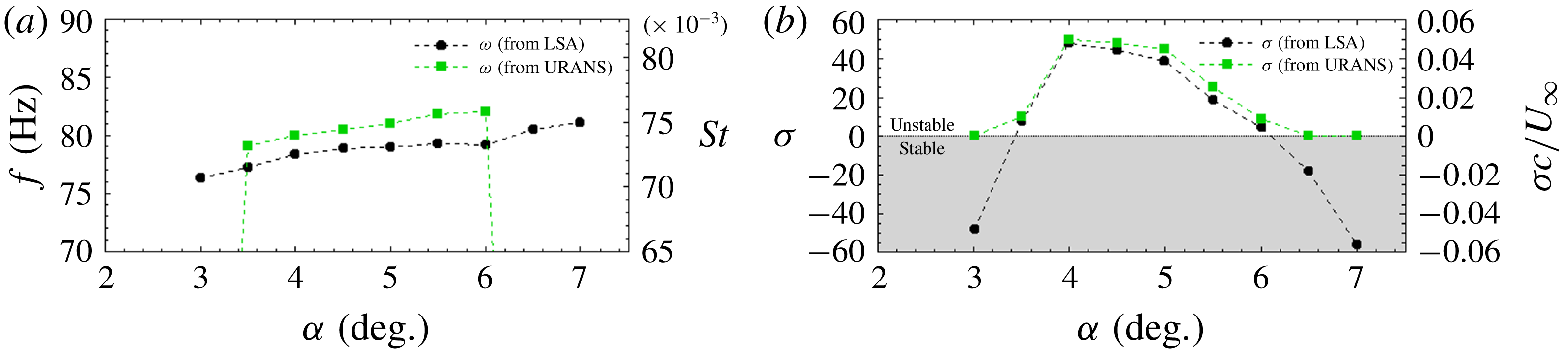
Results of the global stability analysis are presented below with an emphasis on the evolution of the most unstable mode as a function of the angle-of-attack $\unicode[STIX]{x1D6FC}$ for a fixed value of the Mach number $M=0.73$ . The buffet mode is the only unstable global mode in the considered hypothesis and range of parameters. Figure 11 compares angular frequencies and growth rates from URANS simulations and linear stability analysis from buffet onset to buffet exit and shows a good agreement. The frequency increases with $\unicode[STIX]{x1D6FC}$ in the range of frequencies 75-82 Hz, or in the range of non-dimensional frequencies (Strouhal number $St=fL/U$ ) 0.07–0.075, where $f$ is the frequency of the phenomenon and $U$ and $L$ , the reference velocity and length – here the free-stream velocity and the chord of the airfoil, respectively. Figure 11(b) highlights the angle of attacks where the buffet mode is marginally stable: $\unicode[STIX]{x1D6FC}=3.5^{\circ }$ and $\unicode[STIX]{x1D6FC}=6.0^{\circ }$ .

Interesting information comes from the structure of the buffet mode. Both direct and adjoint modes have been computed. Figure 12 shows the real and imaginary parts of both direct and adjoint modes for the $\unicode[STIX]{x1D70C}E$ component. Direct modes exhibit high values at the shock position and in the detached boundary layer; while adjoint modes have high values along the descending characteristic line to the shock foot and the boundary layer upstream of the shock. The present results of global stability analysis agree with Crouch et al. (Reference Crouch, Garbaruk and Magidov2007, Reference Crouch, Garbaruk, Magidov and Jacquin2009a ,Reference Crouch, Garbaruk, Magidov and Travin b ) and Sartor et al. (Reference Sartor, Mettot and Sipp2015).

Figure 11.

Evolution of angular frequency (a) and temporal growth rate (b) with the angle-of-attack for $M=0.73$ for both results of URANS simulations and stability analysis.

Figure 12.

The $\unicode[STIX]{x1D70C}E$ component of the buffet mode at $\unicode[STIX]{x1D6FC}=5^{\circ }$ and $M=0.73$ . (a) Real and (b) imaginary parts of the direct buffet mode. (c) Real and (d) imaginary parts of the adjoint buffet mode. Solid and dashed lines are, respectively, the supersonic region and the boundary layer thickness of the steady state solution.

4.4 Structural sensitivity and decomposition results

The approaches presented above are now applied to the transonic buffet unstable mode. Figure 13(a,b) shows the density maps of the angular frequency and growth rate for buffet mode at $\unicode[STIX]{x1D6FC}=5^{\circ }$ and Mach number $0.73$ . For these values of $\unicode[STIX]{x1D6FC}$ and $M$ , the flow field is in a regime of well-established buffet. The supersonic zone (solid line) and the detached boundary layer (dashed line) of the steady-state solution are also shown in order to compare these density maps with the physics of the flow field. Both growth rate and angular frequency exhibit maximum values around $10^{7}$ at the shock foot (note that the colour maps are exponential). The zoom in figure 13 shows that the region of maximum value is inside the lambda shape of the shock foot where the boundary layer detaches. Lower values of the density maps, around $10^{5}$ , are found along the shock and in the boundary layer. The zone near the shock, above the detached boundary layer and in the wake, exhibits values of growth rate and frequency density of approximately $10^{3}$ . All the other zones have values lower than $10^{2}$ , i.e. $4$ to $6$ orders of magnitude lower than the values at the shock foot. In summary buffet instability appears strongly localized at the shock foot with a smaller contribution of the shock and the separated boundary layer. These results suggest the existence of several zones, even close to the airfoil (for example, the pressure side), that do not impact the physical mechanism at the origin of the transonic buffet. Further investigations are presented here for the density maps of the growth rate. Indeed positive values contribute to the unstable behaviour of the mode while negative values are stabilising. The shock foot always appears with a strongly unstable behaviour while the shock always exhibits a stable behaviour. The detached boundary layer may have either a stable or an unstable behaviour depending on the location in space and the values of the angle-of-attack.

Figure 13.

(a) Growth rate and (b) angular frequency density maps for the buffet mode at $M=0.73$ and $\unicode[STIX]{x1D6FC}=5^{\circ }$ , with a zoom on the shock foot. Solid and dashed lines respectively depict the supersonic region and the boundary layer of the steady state solution.

Figure 14.

Growth rate density maps for the buffet mode at $M=0.73$ and (a)  $\unicode[STIX]{x1D6FC}=3^{\circ }$ , (b)  $4.5^{\circ }$ and (c)  $7^{\circ }$ . Solid and dashed lines are, respectively, the supersonic region and the boundary layer of the steady state solution.

Figures 14(a)–14(c) show the growth rate density maps before buffet onset at $\unicode[STIX]{x1D6FC}=3^{\circ }$ , in a well-established buffet regime at $\unicode[STIX]{x1D6FC}=4.5^{\circ }$ and after buffet exit at $\unicode[STIX]{x1D6FC}=7^{\circ }$ . These three maps show three different regimes of the flow but the summation of all the contributions to the growth rate for figure 14(a,c) is close. Figure 14(b) gives the opposite, strong values of total growth rate. It is now interesting to analyse locally the space distribution of the growth rate for figure 14(a,c). They both show a detached boundary layer with negative values of the density growth rate while figures 14(b) and 13(a), in a condition of well-established buffet, show an area with positive values completely inside the detached boundary layer. In a certain way if the summation of the local contribution is performed by considering only the values inside the detached boundary layer, the result is a negative value for the case in figure 14(a,c) while it is positive for figures 14(b) and 13(a). The analysis of the density maps of the growth rate at different angles of attack suggest that the detached boundary layer has an important role on the buffet instability scenario. At buffet onset the behaviour, in terms of contribution to the growth rate, of the detached boundary layer changes with the appearance of destabilising zones (which disappear at buffet exit) and it can be explained as the active key of buffet instability.

Once the local contributions to the unstable eigenvalue are defined, the other decomposition are now analysed. The multiplicative perturbation approach presented in § 2.4 is straightforwardly deduced from the localized contributions, as for the vortex shedding mode. The multiplicative localized damping maps are deduced from the local contribution by multiplying both maps by the negative scalar $-\unicode[STIX]{x1D712}$ . The result for the growth rate is a strong stabilising damping effect at the shock foot, destabilising on the shock and both effects in the boundary layer. The frequency, as for the vortex shedding mode, is mainly reduced by the multiplicative localized damping.

The attention is now focused on the additive localized damping approach, which could also be deduced from the localized contributions but it will be independently computed and then the link discussed. Figure 15 shows the additive localized damping maps for the buffet mode. As already seen on the vortex shedding mode, these maps are very similar to the local contribution maps, and consequently to the multiplicative localized damping maps as well. The reason could be found in the rate between real and imaginary parts of the eigenvalue, respectively, the growth rate and the frequency. Indeed, near the threshold the frequency of an unstable mode is much higher than its growth rate and the phase of the mode in polar coordinate is close to $\unicode[STIX]{x03C0}/2$ . This is true in the full range of instability for the buffet mode: the lowest value of the phase of the mode in polar coordinates is $0.94\unicode[STIX]{x03C0}/2$ (which corresponds to the highest growth rate). Consequently there is a shift of the maps’ density between the local contribution and the multiplicative localized damping in comparison with the additive localized damping.

The analysis of these maps from the linear stability results in some important contributions to the final definition of the scenario of the physical mechanism behind transonic buffet. The shock foot appears to be the core of the instability and the zone where the unsteadiness arises. The shock has a stabilising behaviour during the unstable phenomenon which can be interpreted as a stiffness (a section of the field that is sustained by, and tends to damp, the shock foot motion). Finally, the detached boundary layer changes its stabilising/destabilising/stabilising behaviour during the stable/unstable/stable phenomenon and consequently it appears to be linked with the onset and exit of buffet. In order to confirm the influence of the different zones in the buffet phenomenon resulting from stability density maps, the local selective filtering method is used in the following.

Figure 15.

Additive localized damping approach on (a) the growth rate and on (b) the frequency for the buffet mode at $M=0.73$ and $\unicode[STIX]{x1D6FC}=5^{\circ }$ , with a zoom on the shock foot. Solid and dashed lines respectively depict the supersonic region and the boundary layer of the steady state solution.

Figure 16.

Zones of the computational domain where SFD is locally activated. Solid and dashed lines are respectively the supersonic zone and the separated boundary layer of the steady state solution. Black points are the probe positions, (a) zone 1, (b) zone 2, (c) zone 3, (d) zone 4, (e) zone $4^{\prime }$ , (f) zone 5, (g) zone 6, (h) zone 7.

4.5 Selective frequency damping

Based on the results obtained in the previous section, eight flow regions are investigated in applying the damping term. They are depicted in figure 16: the suction side of the airfoil (zone 1), the shock foot excursion and beginning of the separated boundary layer (zone 2), the suction side TE area and wake (zone 3), from the superior half of the supersonic zone to the end of the domain (zone 4) above the supersonic zone (zone $4^{\prime }$ ), the airfoil wake (zone $5$ ), the path between the TE and the shock above the boundary layer (zone 6) and finally the pressure side of the airfoil (zone $7$ ). Lift fluctuation amplitudes are used as global criteria for the persistence of the buffet instability. Steady state is defined by zero machine levels of residuals while probes are used locally to verify that unsteady signals are well damped. When lift continues to oscillate and the standard deviations of the signals in the filtered zone tend to zero it is possible to state that the related zone is not necessary for the buffet instability to develop, consequently there is not a critical value of $\unicode[STIX]{x1D712}$ . To choose the SFD parameters, Åkervik et al. (Reference Åkervik, Brandt, Henningson, Hœpffner, Marxen and Schlatter2006) state that large $\unicode[STIX]{x1D712}$ and $\unicode[STIX]{x1D6E5}$ would make the evolution of the system very slow but the SFD would in every case converge to a steady-state. Furthermore, the SFD parameter values are linked to the flow dynamics. The temporal cutoff frequency $1/\unicode[STIX]{x1D6E5}$ should be lower than the frequency of the unstable dynamics by at least a factor two. The control parameter $\unicode[STIX]{x1D712}$ usually has a value close or higher than the growth rate of the unstable flow dynamics but can take higher values in order to increase the convergence rate of the simulation towards the steady-state. In most cases the unstable dynamics is unknown a priori and several studies proposed different techniques to choose suitable parameters (Jordi, Cotter & Sherwin Reference Jordi, Cotter and Sherwin2015; Cunha, Passaggia & Lazareff Reference Cunha, Passaggia and Lazareff2015). In the present work the unstable dynamics is well known and the analysis procedure is the following: eight URANS simulations are performed with SFD for each filtered zone in figure 16, the value of the cutoff frequency is fixed at $13~\text{rad}\cdot \text{s}^{-1}$ , which ensures an efficient convergence for the SFD algorithm and $\unicode[STIX]{x1D712}_{c}\approx \unicode[STIX]{x1D70E}$ when $\unicode[STIX]{x1D644}_{S}=\unicode[STIX]{x1D644}$ . The dependence of $\unicode[STIX]{x1D712}_{c}$ with respect to the choice of $\unicode[STIX]{x1D6E5}$ has also been investigated but is not presented here since only small effects on $\unicode[STIX]{x1D712}_{c}$ have been observed.

As for the implementation of the modified SFD algorithm, the ‘encapsulated’ formulation, described in Jordi, Cotter & Sherwin (Reference Jordi, Cotter and Sherwin2014), is used. It is based on the splitting of the system (2.19) to cope with the industrial CFD solver elsA.

4.5.1 Results

The results from the application of SFD in the different zones are presented in this section. The numerical parameters of the URANS simulations have been described in § 2.1. The configuration analysed is the same as in § 4.4: $(Re,M,\unicode[STIX]{x1D6FC})=(3.2\times 10^{6},0.73,5^{\circ })$ . As already said, the effect of a particular zone on the global instability is assessed through two criteria: a global one based on the lift oscillation amplitude and a local one based on the standard deviation of signals from probes which quantifies how much unsteady signals are damped in the zones where SFD is locally activated.

Once the local SFD is activated, there are two types of results. In the first case a steady-state is reached, residuals decrease towards zero machine values. In the second case a steady-state is not reached. It is then possible to force the convergence towards the steady-state solution by increasing the control parameter $\unicode[STIX]{x1D712}$ , but the achievement of the converged solution depends on the zone where the SFD is activated. Figure 17(a) shows the lift oscillation amplitude for increasing values of the control parameter $\unicode[STIX]{x1D712}$ , for the application of SFD in the entire computational domain and three cases of local application (zones 2, 3 and 4). When $\unicode[STIX]{x1D712}=0$ , the lift oscillation amplitude corresponds to the URANS one without SFD. For increasing values of $\unicode[STIX]{x1D712}$ , the lift oscillation amplitude decreases towards zero, with a slope depending on the zone where SFD is activated. When $\unicode[STIX]{x0394}C_{l}=0$ (corresponding to $\unicode[STIX]{x1D712}_{c}$ ) the residuals’ values tend to zero machine levels while intermediate points, in the range $0<\unicode[STIX]{x1D712}<\unicode[STIX]{x1D712}_{c}$ , correspond to non-physical solutions of the URANS dynamical system coupled with SFD that did not reach convergence. The application of the SFD on the full domain results in a value of $\unicode[STIX]{x1D712}_{c}=55$ , while $\unicode[STIX]{x1D712}_{c}$ is always higher when SFD is applied on a limited zone of the domain. Figure 17(a) shows the regions in which the application of a local SFD allows it to reach a steady-state, for a certain value of $\unicode[STIX]{x1D712}$ . Table 1 shows the $\unicode[STIX]{x1D712}_{c}$ values for the configurations in figure 16. Here ‘N/A’ is used when a value of $\unicode[STIX]{x1D712}_{c}$ is not found, i.e. when SFD damps the entire unsteady signals of the zone where it is activated but the lift still oscillates. A steady-state is reached by application of local SFD only for three zones: shock (zone 4), suction side TE area and wake (zone 3) and shock foot with the beginning of the boundary layer (zone 2) which is the most efficient area to damp. These zones correspond exactly to the higher values of the maps presented in figures 13 and 15. It is interesting to note the low value of $\unicode[STIX]{x1D712}_{c}$ for zone 2 even though the application area of the SFD is very small and that $\unicode[STIX]{x1D712}_{c}$ for zone 1 is very close to the value found when SFD is applied on the entire computational domain.

Figure 17.

(a) Amplitude of lift coefficient oscillation as a function of the control parameter $\unicode[STIX]{x1D712}$ for SFD activated on the entire domain and three local applications, (b) the standard deviation of the streamwise momentum $\unicode[STIX]{x1D70C}u$ as function of the control parameter $\unicode[STIX]{x1D712}$ for the SFD activated on zone 4; for the probes’ location see figure 16(d).

Table 1.

Minimal value of the control parameter $\unicode[STIX]{x1D712}$ to reach a steady state for the different zones where SFD is activated.

The local criterion based on the standard deviation, $sd$ , for the streamwise momentum, $\unicode[STIX]{x1D70C}u$ , is presented for zone 4 in figure 17(b). The same slope is found for all other state variables. For zones 1, 2 and 3, the standard deviation of the state variables decreases constantly while increasing $\unicode[STIX]{x1D712}$ , until $\unicode[STIX]{x1D712}_{c}$ (figure omitted). Four different probes are used in zone 4, two above the supersonic zone and two inside the area swept by the shock. Figure 16(d) shows the location of all the probes. Figure 17(b) shows that the standard deviation of $\unicode[STIX]{x1D70C}u$ drastically decreases when SFD is activated for the probes outside the supersonic zone (probes C and D) while remaining on a plateau and then strongly decreasing to zero for the probes inside the supersonic zone (probes A and B). The results in figure 17(b) suggest that the flow field converges towards a steady state as soon as SFD is activated, except for the shock which continues to oscillate. Damping the perturbations around the shock does not suppress the oscillation. Consequently, the perturbations around the supersonic zone are considered more a consequence than a cause of the buffet. Now, by considering the low value of $\unicode[STIX]{x1D712}_{c}$ for the shock foot, it is possible to give an explanation of the behaviour of the shock in the global instability. It is in a certain way entrained by the core of the instability, the shock foot, but at the same time it has a role in the buffet scenario (it is indeed possible to suppress the instability with a high value of $\unicode[STIX]{x1D712}_{c}$ ). To conclude, the shock is a slave zone but behaves as a stiffness on the instability phenomenon. If some part of the shock is prevented from moving, the rest of the shock, even if it is free to move, has a harder time doing it.

The analysis continues with zones where it is not possible to suppress buffet instability by local SFD. This is the case for zones $4^{\prime }$ , 5, 6 and 7. Figure 18(a) shows the global criterion based on the lift oscillation amplitude as a function of the control parameter $\unicode[STIX]{x1D712}$ for zone 7. For $\unicode[STIX]{x1D712}=6400$ the shock still oscillates even if the lift coefficient amplitude is reduced by approximately $25\,\%$ . At the same time, figure 18(b) shows the local criterion based on the standard deviation for the streamwise momentum, $\unicode[STIX]{x1D70C}u$ , at the point depicted in figure 16(h); it is decreased by $98\,\%$ for the same value of $\unicode[STIX]{x1D712}$ . This indicates that the SFD technique effectively suppresses fluctuations in the region where the filter is applied but the buffet instability is still present. The same conclusion was found in Memmolo et al. (Reference Memmolo, Bernardini and Pirozzoli2018) by freezing the URANS solution on the same zone. To freeze a solution is equivalent to using SFD with a control parameter $\unicode[STIX]{x1D712}=\infty$ . Results for the other zones are not presented because they are very similar to the ones of zone 7. For example zone 6 at $\unicode[STIX]{x1D712}=4000$ shows a reduction of $22\,\%$ in lift coefficient amplitude with a reduction of $98.5\,\%$ in the standard deviation of $\unicode[STIX]{x1D70C}u$ .

Figure 18.

Amplitude of (a) the lift coefficient oscillation and (b) standard deviation of the state variable $\unicode[STIX]{x1D70C}u$ , as function of the control parameter $\unicode[STIX]{x1D712}$ for the SFD activated on zone 7; for the probes’ location see figure 16(h).